HAL Id: hal-00159475
https://hal.archives-ouvertes.fr/hal-00159475
Submitted on 1 Apr 2008
HAL is a multi-disciplinary open access
archive for the deposit and dissemination of
sci-entific research documents, whether they are
pub-lished or not. The documents may come from
teaching and research institutions in France or
abroad, or from public or private research centers.
L’archive ouverte pluridisciplinaire HAL, est
destinée au dépôt et à la diffusion de documents
scientifiques de niveau recherche, publiés ou non,
émanant des établissements d’enseignement et de
recherche français ou étrangers, des laboratoires
publics ou privés.
imaging algorithms applied to short-range UWB
scattering data
Ioannis Aliferis, T. Savelyev, M. Yedlin, Jean-Yves Dauvignac, A. Yarovoy,
Christian Pichot, L. Ligthart
To cite this version:
Ioannis Aliferis, T. Savelyev, M. Yedlin, Jean-Yves Dauvignac, A. Yarovoy, et al.. Comparison of the
diffraction stack and time-reversal imaging algorithms applied to short-range UWB scattering data.
IEEE International Conference on Ultra-WideBand (ICUWB2007), Sep 2007, Singapore, Singapore.
pp.618-621. �hal-00159475�
Comparison of the diffraction stack and
time-reversal imaging algorithms applied to
short-range UWB scattering data
Ioannis Aliferis
∗, Timofey Savelyev
†, Matthew J. Yedlin
∗‡, Jean-Yves Dauvignac
∗,
Alexander Yarovoy
†, Christian Pichot
∗and Leo Ligthart
†∗
LEAT, Universit´e de Nice – Sophia Antipolis, CNRS;
250 rue Albert Einstein, Bˆat 4, 06560 Valbonne, France
†
International Research Center for Telecommunications and Radar, Delft University of Technology,
Mekelweg 4, 2628 CD Delft, the Netherlands
‡
Department of Electrical and Computer Engineering, U.B.C., Canada
Abstract—Comparison of different techniques for short-range
UWB radar imaging has been performed based on experimental data. To acquire experimental data, a video-impulse radar with a specially developed antenna system with a single transmitter antenna and an array of receiver antennas has been used. Topology of the receiver array was made in such a way that the footprint of the receiver array does not have any sidelobes.
Index Terms—Ultra-wideband radar, short-range imaging,
imaging algorithms.
I. INTRODUCTION
Recently, a substantial interest has been paid to radars for imaging of subsurface objects. Ground Penetrating Radar (GPR) and medical imaging are the most common applications [1]. Exact localization of detected inhomogeneities and their characterization requires measurement of the field scattered by the subsurface in numerous positions over a surface, which is implemented so far via mechanical 2D scanning of the area under investigation. The mechanical scanning makes data acquisition very time consuming. Furthermore, it is very diffi-cult to realize conformal mechanical scanning along curved surfaces (as required in medical imaging). These problems might be solved by replacing the mechanical scanning over the area by an electrical scanning of the subsurface with a focused antenna footprint, similar to antenna-beam scanning in far field phased arrays. However, the principal difficulty lies in the fact that the antenna footprint focusing should be achieved in the near field rather than in the far field.
In this paper we present results of our investigations on near-field imaging. Using a previously designed receiver an-tenna array [2] we compare different algorithms for near-field imaging with this array. The measurement configuration is discussed in section II. The simplest imaging algorithm, which is based on data migration (diffraction stack algorithm) is presented in section III. A more complicated algorithm (time reversal algorithm) is described in section IV. Comparison of the algorithm performance is done in section V, Conclusion.
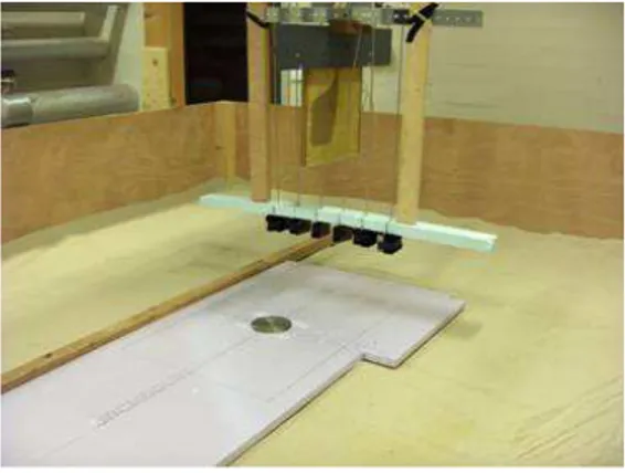
Fig. 1. Measurement configuration: a single transmitter ETS antenna above a receiver array of six loop antennas.
II. MEASUREMENT CONFIGURATION
The measurement configuration is illustrated in Fig. 1. A single transmitter ETS antenna is placed above a linear receiver array of six loop antennas. The height of the phase center of the transmitter antenna above the surface is 43.5 cm and the height of the array is 16.5 cm. The spacing between the loop antennas in the array is 7 cm.
The electronics comprises a signal generator of a 50 ps mono-pulse, and a multi-channel sampling receiver working in a 20 ns time window, i.e. the maximal unambiguous range is 3 m. A detailed description of the hardware design can be found in [2].
A number of various targets were measured. The mea-surement procedure consisted of two steps: (1) background measurement without a target, (2) measurement with a target. Then in processing, the background was subtracted from the target data. For each antenna array element, a 60 cm long B-scan was acquired over the target.
III. COMBINATION OF RECEIVER ARRAY FOCUSING WITH
SAR
TU Delft developed an UWB imaging algorithm combining the focusing within the array aperture and SAR focusing in
Fig. 2. Imaging geometry: origin lies on the phase center of the emitter;
z-axis (vertical distance) points downwards.
the mechanical scan direction [3]. The imaging geometry is presented in Fig. 2. The algorithm can be expressed as follows:
s(xl, ym, zn) = N X k=1 M X j=1 sk(tkj, xl, yj, zn) (1)
where (xl, ym, zn) is a focused grid-point, N is number of
array channels, M is number of measured grid-points in the mechanical scan direction, tkj is a travel time for the
grid-points (xl, yj, zn) for the k-th array channel. This algorithm
uses a diffraction stacking SAR over the line y = xl for
every array channel separately, which accounts for respective time delays, and then sums the weighted channels focused at the point (xl, ym, zn) which is essentially the real aperture
focusing.
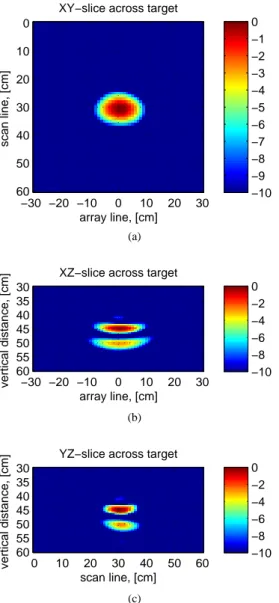
The imaging results for a small metal sphere of 2 cm diameter and for a metal disk of 10 cm diameter are presented in Fig. 3 and Fig. 4 respectively. The targets are shown in three planes in dB scale.
The horizontal slices across the targets (Figs. 3a and 4a) give an estimation of the target size: for the 2 cm sphere we receive about 5 cm at -6 dB level; for the 10 cm disk we receive about 16 cm. Also the presented results show a difference between focusing in the array plane (Figs. 3b and 4b) and SAR in the mechanical scan direction (Figs. 3c and 4c). Due to the larger synthetic aperture and finer measurement grid (1 cm in the algorithm) the focusing in the scan direction is better. The vertical slices (Figs. 3bc and 4bc) reveal multiple images of a target which can be explained by the fact that the transmitted UWB signal has a wavelet-like, bi-polar waveform, consisting of a few periods. When focused, those semi-periods create the respective multiple images.
array line, [cm] scan line, [cm] −30 −20 −10 0 10 20 30 0 10 20 30 40 50 60 −10 −9 −8 −7 −6 −5 −4 −3 −2 −1 0 (a) array line, [cm] vertical distance, [cm]
XZ−slice across target
−30 −20 −10 0 10 20 30 30 35 40 45 50 55 60 −10 −8 −6 −4 −2 0 (b) scan line, [cm] vertical distance, [cm]
YZ−slice across target
0 10 20 30 40 50 60 30 35 40 45 50 55 60 −10 −8 −6 −4 −2 0 (c)
Fig. 3. Image of a 2 cm metal sphere in three planes: (a) in horizontal plane across the sphere, (b) in vertical plane along the receiver array, (c) in vertical plane along the mechanical scan direction.
IV. TIME-REVERSAL PROCESSING OF DATA
The data obtained from the antenna receiver array, recording the scattered waves from several surface targets, illuminated by a single ETS antenna, presents a unique opportunity for testing the time reversal algorithm [4], [5], [6], [7], [8], in a homogeneous background medium, with known propagation speed. Shown in Fig. 5 is an entire background-corrected B-Scan for channel 4 of our antenna array (third antenna from the left in Fig. 1).
For each array antenna at 16.5 cm above the reference plane, we record a complete background field (without target). Then, we record the scattered field from the target (the metallic disk of 10 cm), for all displacements of the array (x-axis) in the
y (scan) direction, over a distance of 60 cm. We subtract the
scattered field from the background field to obtain the field from the scattering target only, under the assumption that it is not coupled directly to any element of the antenna array.
We time-reverse this scattered field data, for a fixed scan
array line, [cm]
scan line, [cm]
XY−slice across target
−30 −20 −10 0 10 20 30 0 10 20 30 40 50 60 −10 −9 −8 −7 −6 −5 −4 −3 −2 −1 0 (a) array line, [cm] vertical distance, [cm]
XZ−slice across target
−30 −20 −10 0 10 20 30 30 35 40 45 50 55 60 −10 −8 −6 −4 −2 0 (b) scan line, [cm] vertical distance, [cm]
YZ−slice across target
0 10 20 30 40 50 60 30 35 40 45 50 55 60 −10 −8 −6 −4 −2 0 (c)
Fig. 4. Image of a 10 cm diameter metal disk in three planes: (a) in horizontal plane across the disk, (b) in vertical plane along the receiver array, (c) in vertical plane along the mechanical scan direction.
0 5 10 −20 0 20 −400 −200 0 200 400 position (cm) time (ns)
Fig. 5. Entire B-scan of the metallic disk for the third antenna from the left in Fig. 1 over the scan line.
in the x-direction, and use the free-space point-source Green’s function to propagate the data back to an assumed target location in the xz plane (the plane that contains the array and is perpendicular to the reference surface in a B-scan geometry). For each assumed target location, we compute the squared magnitude of the total signal, which is essentially the sum of time-reversed, weighted, phase-shifted signals coming from the array antennas. This process yields a two-dimensional magnitude map of possible locations of the scattering source positions in the xz plane and is repeated as the antenna array is moved over the reference plane, along the y direction. Thus, we obtain a data volume comprised of xz images as a function of scan position.
It is important to mention that the above algorithm actually gives a map of the total electric field energy that passes through each pixel during the time-reversed signal propagation. That means that the images we get contain only spatial focusing information with no indication on time focusing.
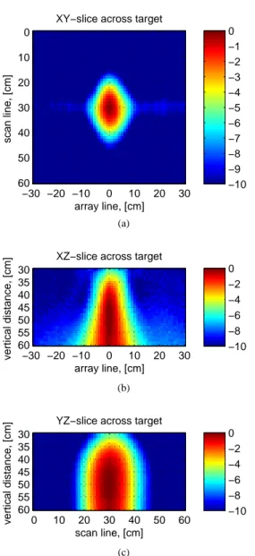
Shown in Fig. 6 are three different slices of the data volume. In Fig. 6a we present a data slice in the xy plane at vertical distance z = 43.5 cm, which corresponds to the reference
surface where the target lies on. The ellipticity is an aperture array effect, along the x direction. Shown in Fig. 6b is an
xz slice (directly obtained from the time-reversal algorithm)
taken directly over the disk location, which corresponds to the scanning position of 223∆y, while in Fig. 6c is shown
a yz slice, taken directly over the disk location, through the center of the array. Both vertical slices show the accumulated electric field energy over the time-reversed signal propagation in free-space. Propagation beyond the z = 43.5 cm plane
(reference surface) is obviously fictitious and must not be taken into account. The time-reversal algorithm (xz slice, Fig. 6b) focuses the energy on the scatterer, but successive TR slices along the scan line (yz slice, Fig. 6c) give similar results in the vicinity of the scatterer, thus resulting to a less focused pattern — this explains the ellipticity in Fig. 6a.
The main result here is that the maximum energy in every slice in Fig. 6 is in the vicinity of the target (centered at
(x, y) = (0, 30) cm and lying on the plane z = 43.5 cm) if
we neglect vertical slices beyond the reference surface. The foregoing time-reversal processing represents the first step in the analysis of this scattering data and has been done plane-by-plane in the B-scan configuration. However, there are clearly plane arrivals that also contribute. These out-of-plane arrivals are important and if neglected, also contribute to image blurring [9]. We propose therefore to extend the algorithm defined previously: for each B-scan, we will apply the algorithm to the complete volume of possible scatterers. As there are 447 scans and 6 antennas, it is clear that an optimization of the algorithm will be necessary to achieve the complete image. The complete time-reversal algorithm in 3D, optimized for the entire image volume, is summarized as follows:
1) For all B-scan positions and for each receiving antenna, reflect the data about t= 0.
2) For each image point (volume element) For all receiving antenna positions
array line, [cm] scan line, [cm] −30 −20 −10 0 10 20 30 0 10 20 30 40 50 60 −10 −9 −8 −7 −6 −5 −4 −3 −2 −1 0 (a) array line, [cm] vertical distance, [cm]
XZ−slice across target
−30 −20 −10 0 10 20 30 30 35 40 45 50 55 60 −10 −8 −6 −4 −2 0 (b) scan line, [cm] vertical distance, [cm]
YZ−slice across target
0 10 20 30 40 50 60 30 35 40 45 50 55 60 −10 −8 −6 −4 −2 0 (c)
Fig. 6. Image of a 10 cm metal disk in three planes: (a) in horizontal plane across the disk, (b) in vertical plane along the receiver array, (c) in vertical plane along the mechanical scan direction.
b) Weight data and time-shift according to distance and known wave speed;
c) Accumulate, weighted, time-shifted antenna data; Differentiate the accumulated signal, take its magni-tude and assign it to image point.
3) Plot the volume data and take colored slices to view image.
In this way, we can obtain a complete three dimensional image of the scatterers without knowing a priori their location.
V. CONCLUSION
In this paper we have investigated the imaging capabilities of two different UWB imaging algorithms applied to data acquired with an UWB antenna array. We have also presented an optimized algorithmic extension to three dimensions of the time-reversal imaging method, created as a mapping from the three-dimensional data volume to the three-dimensional image volume.
algorithms yields similar results, if properly interpreted. The first algorithm applied is a diffraction stack for a fixed re-ceiving antenna along the scan direction, y, while the second algorithm is a time-reversal algorithm applied in the perpen-dicular direction, along the array direction, x. A graphical comparison of Fig. 4a, through the disk, and Fig. 6a through the plane z= 43.5 cm, which corresponds to the surface where
the target lies on, shows the same elliptical disk, with the ellipticity an aperture effect. The vertical slices (4bc and 6bc) seem different due to the fact that the time-reversal algorithm presented here shows the path of the electric field energy, as discussed in section IV: we see the energy flowing from the antennas toward the object and then continuing artificially below the surface. Temporal focusing, not shown here, will be included in future work together with further comparison on various targets.
ACKNOWLEDGMENTS
The authors wish to acknowledge the assistance and support of ACE activities on GPR antennas by Peter Balling, activity leader for ACE WP2.3. The joint activities have been partly financially supported by European Commission within the FP6 Network of Excellence ACE2 (contract 026957). Data for Fig. 6 were kindly provided by Anthony Cresp, MSc student at LEAT.
REFERENCES
[1] D. J. Daniels, Ground Penetrating Radar, 2nd ed., ser. IEE Radar, Sonar, Navigation and Avionics Series. London: The Institution of Electrical Engineers, 2004, no. 15.
[2] A. Yarovoy, P. Lys, P. Aubry, T. G. Savelyev, and L. P. Ligthart, “Near-field focusing within a UWB antenna array,” in European Conference
on Antennas and Propagation (EuCAP 2006), Nice, France, November
6–10, 2006, pp. 104–105.
[3] T. G. Savelyev, A. Yarovoy, and L. P. Ligthart, “Weighted near-field focusing in an array GPR for landmine detection,” in International
Symposium on Electromagnetic Theory (URSI EMT-S 2007), Ottawa,
Canada, July 26–28, 2007, submitted.
[4] M. Fink, D. Cassereau, A. Derode, C. Prada, P. Roux, M. Tanter, J.-L. Thomas, and F. Wu, “Time-reversed acoustics,” Reports on Progress in
Physics, vol. 63, no. 12, pp. 1933–1995, December 2000.
[5] M. Fink and C. Prada, “Acoustic time-reversal mirrors,” Inverse Problems, vol. 17, no. 1, pp. R1–R38, February 2001.
[6] C. Prada and M. Fink, “Eigenmodes of the time reversal operator: A solution to selective focusing in multiple-target media,” Wave Motion, vol. 20, no. 2, pp. 151–163, September 1994.
[7] C. Prada, S. Manneville, D. Spoliansky, and M. Fink, “Decomposition of the time reversal operator: detection and selective focusing on two scatterers,” Journal of the Acoustical Society of America, vol. 99, no. 4, pp. 2067–2076, April 1996.
[8] M. E. Willis, R. Lu, X. Champman, M. Nafi Toks ¨oz, Y. Zhang, and M. V. de Hoop, “A novel application of time-reversed acoustics: Salt-dome flank imaging using walkaway VSP surveys,” Geophysics, vol. 71, no. 2, pp. A7–A11, March-April 2006.
[9] W. S. French, “Two-dimensional and three-dimensional migration of model-experiment reflection profiles,” Geophysics, vol. 39, no. 3, pp. 265– 277, June 1974.