HAL Id: hal-02127752
https://hal.archives-ouvertes.fr/hal-02127752
Submitted on 13 May 2019
HAL is a multi-disciplinary open access
archive for the deposit and dissemination of
sci-entific research documents, whether they are
pub-lished or not. The documents may come from
teaching and research institutions in France or
L’archive ouverte pluridisciplinaire HAL, est
destinée au dépôt et à la diffusion de documents
scientifiques de niveau recherche, publiés ou non,
émanant des établissements d’enseignement et de
recherche français ou étrangers, des laboratoires
Appropriate analysis of the four-bar linkage
Joshua K. Pickard, Juan Carretero, Jean-Pierre Merlet
To cite this version:
Joshua K. Pickard,
Juan Carretero,
Jean-Pierre Merlet.
Appropriate analysis of the
four-bar linkage.
Mechanism and Machine Theory,
Elsevier,
2019,
139,
pp.237-250.
Appropriate Analysis of the Four-Bar Linkage
Joshua K. Pickarda,∗, Juan A. Carreterob, Jean-Pierre Merletc
aAuctus project, INRIA Bordeaux Sud-Ouest, France
bDepartment of Mechanical Engineering, University of New Brunswick, Fredericton, New
Brunswick, Canada
cHephaistos project, Universit´e Cˆote d’Azur, INRIA, France
Abstract
Uncertainties are inherent in the fabrication and operation of mechanisms. In terms of the four-bar linkage, uncertainties in the geometric parameters result in non-exact solutions for the coupler point. A design description which accounts for bounded uncertainties is termed an appropriate design. Appropriate anal-ysis routines are analanal-ysis routines for guaranteeing that specific requirements will be satisfied, which is applicable to mechanisms described by an appropriate design. These routines rely on interval analysis to provide reliable results and are able to handle the uncertainties present in a mechanism. An appropriate analysis routine which is able to determine the worst-case bounds of the coupler curve resulting from uncertainties is proposed. As well, routines are introduced for evaluating the classification and assembly of mechanisms with uncertainties. Examples are presented to demonstrate the coupler curves of four-bar linkages described by an appropriate design which corresponds to each linkage classifi-cation, including folding linkages.
Keywords: Uncertainties, Interval Analysis, Design, Linkage
1. Introduction to Linkage Design
The four-bar linkage is a planar mechanism consisting of four rigid members: the frame, the input link, the output link, and the coupler link. These members are connected by four revolute pairs forming a closed-loop kinematic chain of 1-degree-of-freedom. A point on the coupler, known as the coupler point, traces a path as the input link is rotated. This path is known as the coupler curve, which is, in general, an algebraic curve of degree six. Useful coupler curves can be generated when the geometric parameters of the linkage are properly selected.
∗Corresponding author
Email addresses: [email protected] (Joshua K. Pickard),
[email protected] (Juan A. Carretero), [email protected] (Jean-Pierre Merlet)
The performance of a linkage cannot be reliably reported using conventional analysis techniques, as these techniques are unable to account for the uncertain-ties inherent in mechanisms. The issue of uncertainuncertain-ties plays a significant role in the actual performance of a mechanism. In the four-bar linkage, uncertainties make it no longer possible to obtain an exact solution for the coupler point. Instead, the coupler point can only be determined to lie within some region, which is a function of the uncertainties.
Several works appear in the literature for analyzing the designs of mecha-nisms while accounting for uncertainties. Ting et al. [1] present an approach for identifying the worst-case positioning errors due to uncertainties in the joints of linkages and manipulators. Chen et al. [2] studied the accuracy performance of general planar parallel manipulators due to input uncertainties and joint clear-ances. Ting et al. [3] studied the effect of joint uncertainties in linkages contain-ing revolute and prismatic joints. In [4], Merlet and Daney consider the error analysis problems applied to a Gough platform. The authors determine the ex-tremal positioning errors corresponding to some specific geometrical parameters which contain uncertainties. In [5], Hao and Merlet present an approach to syn-thesize the complete set of design solutions which satisfy multi-criteria require-ments. The term appropriate design was introduced by Merlet and Daney [6] for the analysis and synthesis of parallel manipulators with bounded uncertain-ties, which take into account any uncertainties present in the mechanism (e.g., manufacturing, assembly, sensors) and satisfy some desired characteristics of the mechanism.
An appropriate design will be used to describe a mechanism whose descrip-tion contains uncertainties. This descripdescrip-tion allows any uncertainties due to the manufacturing, assembly, sensors, and control to be accounted for. The analy-sis or syntheanaly-sis of an appropriate design are then fittingly termed appropriate analysis and appropriate synthesis, respectively. In this work, the appropriate analysis of the four-bar linkage described by an appropriate design is primarily considered.
The contributions of this work are as follows. The kinematic equations are formulated using a coordinate representation, such that the system is well suited for interval analysis. Linkage classification and linkage assembly routines are proposed which are applicable to appropriate designs. An appropriate analysis routine for obtaining the coupler curves of four-bar linkages described by an appropriate design is proposed. This routine determines a region, which will be a union of boxes, that is guaranteed to contain all possible coupler curves of the appropriate design, whatever the design parameters. The routine is used to obtain the associated coupler curves for each classification of four-bar linkage, including folding linkages.
The outline of the paper is as follows. First, in Section 2, fundamental con-cepts and tools in interval analysis are briefly presented. More specifically, the interval framework, including notation and methods, that are utilized through-out this work are presented. Throughthrough-out the remainder of the work, it will be assumed that the reader has a working knowledge of interval analysis (see [7, 8, 9, 10]). The description of the four-bar linkage and accompanying
kine-matic equations are provided in Section 3. As well, the linkage classification and linkage assembly routines are presented. Then an appropriate analysis routine is presented in Section 4 for computing an outer approximation of the coupler curve associated with a given appropriate design, and associated coupler curves for each classification of four-bar linkage are presented. Finally, the work is concluded in Section 5.
2. Fundamentals of Interval Analysis
Interval arithmetic and interval analysis provide a means of performing re-liable computations on computers. It is a well-known issue that the floating point representation used by computers has a finite set of values that can be represented exactly. All other values can only be approximated. An insightful quote regarding interval analysis was made by Hayes [11]: “give a digital com-puter a problem in arithmetic, and it will grind away methodically, tirelessly, at gigahertz speed, until ultimately it produces the wrong answer”. Interval arithmetic does not directly improve the accuracy of the calculation, but rather provides a certificate of accuracy by providing guaranteed bounds on the solu-tions. That is, parameters are represented by intervals (e.g., [x] = [x, x]), where interval computations then provide guaranteed bounds on the solution over the domain of each of the parameters. An additional benefit of interval arithmetic on conventional digital computers is that uncertainties in the representation of the parameters can automatically be taken into account.
Allow the width of an interval to be given by
width([x]) = x − x (1)
The midpoint of an interval is given by
mid([x]) = x + width([x])/2 (2)
Let [x] denote an interval vector. The interval evaluation of a function f ([x]) yields the inclusion function [f ], such that f ([x]) is contained inside of [f ]. That is,
f ([x]) = {f (x) | x ∈ [x]} ⊆ [f ]. (3) The bounds of [f ] may be inflated due to two well-known properties of interval analysis. First, the wrapping effect is a result of the axis-aligned representation of intervals. The inclusion function [f ] will always be an axis-aligned box which contains f ([x]) and therefore introduces overestimation to the solution domain. For example, the smallest interval which can represent a circle using Cartesian coordinates is the axis-aligned square with edges tangent to the circle. Over-estimation is inherent in such a representation but may change according to the representation (e.g., there is no wrapping of a circle in polar coordinates). Second, the dependency problem is a result of multiple occurrences of a variable appearing in the equation. This causes additional expansion of the solution do-main since interval arithmetic considers each occurrence as independent. That
is, from the point of view of interval arithmetic, xx is the same as xy. As such, if x = [−1, 1], then xx = [−1, 1] · [−1, 1] = [−1, 1]. Alternatively, if the same operation is represented as x2, there is only a single occurrence of x and the computation is now x2= [−1, 1]2= [0, 1]. It is possible to reduce the effects of the dependency problem by properly writing the equation in a form best suited for interval analysis. For example, the equation x2+ 2x + 1 may be changed to (x+1)2to remove an occurrence of x. It is important to note that the amplitude of the overestimation of [f ] decreases with the width of [x] due to the inclusion isotonicity of interval arithmetics (see [7]).
An interval analysis solving routine generally contains three phases evaluated in a loop: simplification, existence, and bisection. Let [k] denote the known variables and [u] denote the unknown variables in a problem and let f ([u], [k]) = 0 be the system being solved. The following subsections elaborate on each of the three phases and how an interval solving routine incorporating all three can be formulated.
2.1. Simplification
In the simplification phase, various heuristic routines (e.g., 2B and 3B filter-ing [12], HC4 [13], ACID [14], Newton [7]) can be applied to attempt to reduce the width of the unknowns [u], such that they become more consistent with the knowns [k] for the system f ([u], [k]) = 0. Consistency is described by the tightness of the unknowns to the actual solution.
As an example, consider solving the equation 3x2+x+1 = 0 with x ∈ [−3, 3]. The 2B filtering method considers rewriting the equation as x = −3x2− 1 which gives the interval [−28, −1] for the right-hand side. The value of x is simplified by taking [−3, 3]∩[−28, −1] = [−3, −1]. Using this new value for x and the same process leads to the right-hand side interval [−28, −4] which has no intersection with [−3, −1] so that the equation has no solution for x ∈ [−3, 3].
An unknown [ui] is considered to be simplified if the width is reduced. If any unknown is simplified to an empty set, then no solution exists for the unknowns. A simplification procedure returns the outcome of the simplification as:
−1 : no solution exists in [u]; 1 : [u] has been simplified; 0 : [u] has not been simplified.
A function SIMPLIFICATION([u], [k]) applies one or more simplification meth-ods to the unknowns [u] together with the evaluation of f ([u], [k]). Simplification may be repeated as many times as desired, usually until significant simplification can no longer be achieved.
2.2. Existence
In the existence phase, existence methods (e.g., Interval Newton [15], Kraw-cyzk [7], Newton-Kantorovitch [16]) are applied to determine if a unique solu-tion [u∗] exists within the domains of the unknowns [u] which correspond to the
knowns [k] for the system f ([u], [k]) = 0. Associated to these methods are solv-ing algorithms, ussolv-ing either only the Jacobian matrix of the system or both the Jacobian and Hessian matrices, that are guaranteed to converge to the unique solution, where a unique solution corresponds to a region of non-separable so-lutions. The existence methods may also return that no solution exists. An existence method returns the outcome of the existence test as:
−1 : no solution exists in [u]; 1 : a unique solution [u∗] is found;
0 : otherwise (additional bisection/analysis is required)
A return value of 0 means that interval analysis is unable to safely determine if there are solutions or not and may be a consequence of the wrapping effect and dependency problem. The function EXISTENCE([u], [k]) applies an existence method to the unknowns [u].
2.3. Bisection
In the bisection phase, the range of one of the unknowns [ui] is bisected such that the original unknowns [u] are split into two subintervals [u1] and [u2]. The union of the two subintervals results in the original interval, thus no combination of unknowns are skipped. A common stopping criteria is to exit when the width of all unknowns are less than a desired threshold β. It is required, however, to maintain a list of the bisected interval vectors, denoted Lu. Many methods have been proposed for choosing the variable whose range will be bisected, and while there is currently no optimal technique, the following techniques are usually selected and are used in this paper.
• Largest-first – [u] is bisected along dimension i such that [ui] is the interval which has the largest width. The bisection usually splits [u] along the midpoint of the interval [ui]. This technique suffers when the unknowns contain different units and therefore may require the parameters to be non-dimensionalized.
• Smear function (introduced by Kearfott [17]) – let Jji be the jth row and ith column of the Jacobian evaluated over [u]. The smear value si is evaluated for each unknown i as
si= max(|Jji[ui]|) ∀j ∈ [1, . . . , n] (4) The unknown [ui] with the largest smear value is selected for bisection, as it is considered as the more sensitive parameter comparatively.
The bisection of an unknown [ui] is only applied when width([ui]) > β. The function BISECTION([u], β) attempts to apply a bisection technique to the unknowns [u]. A successful bisection returns the two subintervals, while an unsuccessful bisection returns nothing. Alternatively, the original interval of an unsuccessful bisection may be saved for later processing.
2.4. Interval Analysis Solving Routine
It is quite straight-forward to create a general interval analysis solving rou-tine. The initial domain of each of the unknowns is added to a list Lu. Given the system f ([u], [k]) = 0, the simplification, existence and bisection phases are applied to each element in the list Lu. This creates a loop since the bisection phase is able to add new boxes to Lu while the original box is eliminated from Lu. To avoid memory issues due to a large number of boxes, a depth-first search is preferable, where new boxes are pushed to the front of list Lu and the next box is always the first box in the list. The size of Lu remains quite small so that memory is not an issue. The loop repeats until the list Luis empty.
It is theoretically possible that in a floating point implementation a box is never eliminated. Indeed if an interval is reduced to [a, a] where a and a are the closest floating point values, then such an interval cannot be further bisected. This case denotes a generically ill-conditioned case and cannot be solved without going to multi-precision arithmetic and are flagged as such. In practice, the algorithms always complete properly. The goal is to determine the list of unique solutions Lu∗ for the unknowns. The known variables [k] are simply considered
as fixed during the solving routine. The method is summarized in Algorithm 1. The bisection resolution β = 0.005 is used throughout.
Algorithm 1: General solving routine function GENERAL SOLVE ([u], [k], β);
Input : unknowns [u], knowns [k], and desired bisection resolution β Output: the list of solutions Lu∗for the unknowns
Lu← [u] ; /* Add unknowns to list Lu */ while Lu is not empty do
Pop unknowns [u] from Lu;
simp = SIMPLIFICATION([u], [k]) ; /* Apply simplification routines */ if simp! = −1 then
exist = EXISTENCE([u], [k]) ; /* Apply existence routines */ if exist == 1 then
Lu∗← [u];
else if exist == 0 then
Lu← BISECTION([u], β) ; /* Apply bisection routine */
3. Four-bar Linkage Description
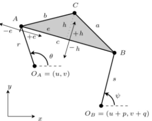
The four-bar linkage and its associated design parameters are provided in Figure 1. The fixed base location OAis located at coordinates (u, v) with respect to the reference frame. The location OB is located at coordinates (p, q) with respect to OA or (u + p, v + q) with respect to the reference frame. Link OAA will always be assumed to be the input link with an input angle θ and length r. Link OBB is the output link, which has an output angle ψ and length s. The coupler point is denoted C = (Cx, Cy), where the coupler link is triangle ABC with edge lengths a, b, and c. The parameters e and h are used to describe the location of C relative to segment AB. The signs of e and h are important to describe a unique assembly of the linkage.
Figure 1: Linkage description
The equations describing the kinematics of the four-bar linkage can be for-mulated by solving a set of distance equations (f1 through f5). The vertex A = (Ax, Ay) of the coupler triangle lies on the circle centred at OAwith radius r. The vertex B = (Bx, By) of the coupler triangle lies on the circle centred at OB with radius s. The points A and B are separated by distance c. The points A and B are functions of the design parameters and input and output angles θ and ψ (f6 through f9). The edg e lengths a and b of the coupler link are functions of the design parameters c, e, and h (f10and f11). The equations f3, f4, f5 alone cannot specify a unique assembly of the linkage and it is therefore necessary to add the constraints f13and f14 which take into account the signs of e and h. For example, in Figure 1, the assembly of the coupler link is con-strained by positive e and h. Changing the sign of h will flip the coupler link and result in a different assembly without changing the link geometry. Finally, let g be the distance between points OA and OB (f12).
f1:= ||OAA||2= (u − Ax)2+ (v − Ay)2= r2
f2:= ||OBB||2= ((p + u) − Bx)2+ ((q + v) − By)2= s2 f3:= ||AB||2= (Ax− Bx)2+ (Ay− By)2= c2
f4:= ||AC||2= (Ax− Cx)2+ (Ay− Cy)2= b2 f5:= ||BC||2= (Bx− Cx)2+ (By− Cy)2= a2 f6:= Ax= u + r cos(θ) f7:= Ay= v + r sin(θ) f8:= Bx= (p + u) + s cos(ψ) f9:= By= (q + v) + s sin(ψ) f10:= b = p e2+ h2 f11:= a = p (c − e)2+ h2 f12:= g =pp2+ q2
f13:= Cx= Ax+ 1/c ((Bx− Ax)e + (Ay− By)h) f14:= Cy= Ay+ 1/c ((By− Ay)e + (Ax− Bx)h)
(5)
The equations f1 through f12 in (5) may be simplified leaving a system of 3 equations with 11 variables. That is,
||AB||2= (r cos(θ) − p − s cos(ψ)))2+ (r sin(θ) − q − s sin(ψ))2= c2 ||AC||2= (u + r cos(θ) − Cx)2+ (v + r sin(θ) − Cy)2= e2+ h2
||BC||2= (p + u + s cos(ψ) − Cx)2+ (q + v + s sin(ψ) − Cy)2= (c − e)2+ h2 (6) This results in a more compact description of the system. However, this com-pact form is not ideal for interval analysis since there are repetitions of variables in each equation. The dependency problem with interval analysis will overes-timate the solution to the system. It is preferable to model the system as (5) since the equations are simpler and yield more efficient simplification procedures and therefore interval analysis methods will be more effective (interval analy-sis requires a trade-off between the number of equations and their complexity). The Jacobian and Hessian matrices generated from equations in (5) are notably simpler, which also have an impact on the efficiency of the existence procedures.
3.1. The Design Parameters
The design parameters of the four-bar linkage given by system (5) are de-scribed by the interval vector [d]:
[d] = ([u], [v], [p], [q], [r], [s], [c], [e], [h])T (7) The interval domains of the parameters account for bounded uncertainties. The manufacturing uncertainties for the design parameters are described by the vec-tor ∆d as
If an exact design d is considered, the appropriate design which accounts for manufacturing uncertainties is given as
[d] = d ± ∆d (9)
Note that using intervals for describing the uncertainties is more realistic than using a statistical distribution that is not related to the physics of the system. Interval analysis is also able to manage the worst-case, which is critical for a failure-safe system.
3.2. Classifications
Four-bar linkages can be sorted into two categories, Grashof-type and non-Grashof-type linkages. Grashof linkages satisfy the Grashof condition, which states that if the sum of the shortest and longest link is less than or equal to the sum of the remaining two links, then the shortest link can rotate fully with respect to a neighbouring link, whereas the links of a non-Grashof linkage cannot rotate fully. Grashof-type linkages and non-Grashof-type linkages each have four different classifications which describe the ranges of the input and output angles. The term crank denotes a link which is able to rotate fully, while the term rocker denotes a link that cannot rotate fully. A double-crank /double-rocker is a linkage whereby both the input and output links are cranks//double-rockers. For non-Grashof linkages, the input and output links will rock through 0 or π. McCarthy and Song Soh [18] describe a routine for classifying a four-bar linkage based only on the length of the links. Their routine may be extended to accept interval design parameters so that uncertainties in the design parameters can be managed. Three interval parameters ([T1], [T2], and [T3]) may be used to identify the possible classifications and are evaluated as
T1= g − r + c − s T2= g − r − c + s T3= −g − r + c + s
(10)
The classification of the linkage is determined from the sign of the three parameters as sgn([T1]) sgn([T2]) sgn([T3]) Classification Type + + + crank-rocker Grashof + - - rocker-crank Grashof - - + double-crank Grashof - + - double-rocker Grashof - - - 00-double-rocker Non-Grashof + + - 0π-double-rocker Non-Grashof + - + π0-double-rocker Non-Grashof - + + ππ-double-rocker Non-Grashof
A folding linkage occurs when any one of the interval parameters ([T1], [T2], or [T3]) includes zero. Such a linkage may be able to take on a configuration
where points OA, OB, A and B lie on a line. This is nearly impossible to achieve physically without flexible links or play in the joints, as the uncertainties prevent such a scenario. Additionally, uncertainties in the design parameters may result in uncertainty in the linkage classification. Therefore, it is necessary to account for uncertainties in the design parameters to ensure that a mechanism will always have a correct classification and be able to perform as desired.
3.3. Branches and Circuits
The description for circuits and branches are adopted from Chase and Mirth [19]. For a given assembly of a four-bar linkage, the coupler point will follow what is referred to as a circuit. In order to change the circuit being fol-lowed, the linkage would need to be disassembled and reassembled. The term toggle position can be used to describe positions which result in collinearity of the coupler and output links. At a toggle position, the linkage is able to change its branch (a branch is defined by a transmission angle, the angle between the coupler and output links, in the range of [0, π] or [−π, 0]) and the branch that will be followed is unpredictable as it depends on the dynamics of the system.
Schr¨ocker et al. [20] describe the number of circuits corresponding to a par-ticular classification of linkage. The ranges of the input and output angles corresponding to a particular classification are given by McCarthy and Song Soh [18]. Note that the vector OAOB is used as a reference for the angles in [18]. Here, the angles must be shifted such that
θ0= θ − atan2(q, p)
ψ0= ψ − atan2(q, p) (11) The limits on the angles are determined as follows
θ0min= acos((g2+ r2) − (c − s)2)/(2rg) θmax0 = acos((g2+ r2) − (c + s)2)/(2rg) ψ0min= acos((c + r)2− (g2+ s2))/(2sg) ψmax0 = acos((c − r)2− (g2+ s2))/(2sg)
(12)
A branch is identified from the transmission angles. Let T1 and T2 denote transmission angles in the ranges [0, π] and [−π, 0] respectively. The conditions for each branch consider the sign of the cross product of the coupler link and output link as
T1:= cos(ψ)(r sin(θ) − q) + sin(ψ)(−r cos(θ) + p) > 0
T2:= cos(ψ)(r sin(θ) − q) + sin(ψ)(−r cos(θ) + p) < 0 (13)
The circuit and branch conditions are described as follows.
• crank-rocker (2 circuits, each with 1 branch): 1. θ0 ∈ [0, 2π], ψ0
2. θ0 ∈ [0, 2π], −ψ0
max≤ ψ0 ≤ −ψ0min, T1 or T2 • rocker-crank (2 circuits, each with 2 branches):
1. ψ0 ∈ [0, 2π], θ0 min≤ θ0≤ θ0max, T1 2. ψ0 ∈ [0, 2π], θ0 min≤ θ0≤ θ0max, T2 3. ψ0 ∈ [0, 2π], −θ0 max≤ θ0 ≤ −θmin0 , T1 4. ψ0 ∈ [0, 2π], −θ0 max≤ θ0 ≤ −θmin0 , T2 • double-crank (2 circuits, each with 1 branch):
1. θ0 ∈ [0, 2π], ψ0∈ [0, 2π], T1 2. θ0 ∈ [0, 2π], ψ0∈ [0, 2π], T
2
• double-rocker (2 circuits, each with 2 branches): 1. θ0min≤ θ0≤ θ0
max, ψ0min≤ ψ0 ≤ ψmax0 , T1 2. θ0min≤ θ0≤ θ0
max, ψ0min≤ ψ0 ≤ ψmax0 , T2 3. −θ0
max≤ θ0≤ −θmin0 , −ψmax0 ≤ ψ0 ≤ −ψ0min, T1 4. −θ0max≤ θ0≤ −θ0
min, −ψmax0 ≤ ψ0 ≤ −ψ0min, T2 • 00-double-rocker (1 circuit with 2 branches):
1. −θ0max≤ θ0≤ θ0
max, −ψmax0 ≤ ψ0≤ ψ0max, T1 2. −θ0max≤ θ0≤ θ0max, −ψmax0 ≤ ψ0≤ ψ0max, T2 • 0π-double-rocker (1 circuit with 2 branches):
1. −θ0
max≤ θ0≤ θ0max, ψmin0 ≤ ψ0 ≤ 2π − ψ0min, T1 2. −θ0max≤ θ0≤ θ0
max, ψmin0 ≤ ψ0 ≤ 2π − ψ0min, T2 • π0-double-rocker (1 circuit with 2 branches):
1. θ0min≤ θ0≤ 2π − θ0
min, −ψ0max≤ ψ0≤ ψ0max, T1 2. θ0min≤ θ0≤ 2π − θ0
min, −ψ0max≤ ψ0≤ ψ0max, T2 • ππ-double-rocker (1 circuit with 2 branches):
1. θ0
min≤ θ0≤ 2π − θ0min, ψmin0 ≤ ψ0≤ 2π − ψ0min, T1 2. θ0min≤ θ0≤ 2π − θ0
min, ψmin0 ≤ ψ0≤ 2π − ψ0min, T2
To determine the circuit, it is also necessary to know which side of the line AB the coupler point is on. That is, h ≥ 0 corresponds to one circuit, whereas h < 0 corresponds to another circuit. Therefore, depending on the assembly and classification of the linkage, there may be at most two circuits and each circuit may have at most two branches. In the following sections, each circuit and branch pair are identified with unique colours.
3.4. Solving the Kinematics
To solve the kinematics of the four-bar linkage in this work, a problem, termed the forward problem, may be considered for appropriate analysis:
• Forward problem: Determine a solution for the coupler point ([Cx], [Cy]) for a fixed value for [θ] and an allowable range for [ψ]. For this problem, a fixed value for [θ] is given and [ψ] is given as an allowable range. The goal is to compute all solutions for ([Cx], [Cy]) and [ψ] which correspond to the fixed value of [θ].
The forward problem is useful for computing the coupler curve associated with an appropriate design. To solve this, an existence test can be formulated from Equations f2–f5. This gives a square system in unknowns Bx, By, Cx, and Cy. The Jacobian matrix J and Hessian matrix H of the corresponding system with these unknowns are
J = −2p − 2u + 2Bx −2q − 2v + 2By 0 0 −2Ax+ 2Bx −2Ay+ 2By 0 0
0 0 −2Ax+ 2Cx −2Ay+ 2Cy 2Bx− 2Cx 2By− 2Cy −2Bx+ 2Cx −2By+ 2Cy
(14) H = 2 0 0 0 2 0 0 0 0 0 0 0 2 0 −2 0 0 2 0 0 0 2 0 0 0 0 0 0 0 2 0 −2 0 0 0 0 0 0 0 0 0 0 2 0 −2 0 2 0 0 0 0 0 0 0 0 0 0 0 0 2 0 −2 0 2 T (15) The elements in the Jacobian matrix do not have repeated variables, making the formulation ideal for interval analysis. Furthermore, the optimal evaluation of the Jacobian elements allows one to check the monotonicity of an equation with respect to the variables. If an equation is monotonic it allows for a better interval evaluation of the equation. As well, the Hessian matrix is constant and therefore does not need to be recomputed. To create various solving routines, a bisection phase may safely bisect the input and/or output angles [θ] and [ψ].
4. Coupler Curve
The coupler curve may be obtained for an appropriate design using an appro-priate analysis routine. Given an approappro-priate design of a linkage, it is desirable to determine the set of boxes which tightly contain the coupler curve. This provides a description of the worst-case error in the coupler curve. If the set of boxes, pertaining to some portion of the coupler curve are contained inside a desired response, then it is possible to state that the linkage design satisfies the desired response. Thus, appropriate analysis may be used for the certification of mechanisms.
The appropriate analysis routine in Algorithm 2 solves for the set of coupler point intervals ([Cx], [Cy]) using the forward problem formulation. Let ∆θ rep-resent the desired resolution of the input angle. A loop iterates over all values
of [θ] in the range [0, 2π]. Inside this loop, the general solving routine returns the list of solution coupler points which correspond to [θ] (boundary points may also be saved). The unknowns and knowns inside the general solving routine are [u] = ([Bx], [By], [Cx], [Cy]) and [k] = ([d], [Ax], [Ay]). The solving rou-tine returns the list of solutions and boundaries as Lu∗. These solutions may
correspond to different assemblies.
Algorithm 2: Coupler curve routine function COUPLER CURVE ([u], [k], ∆θ, β);
Input : unknowns u, knowns k, angle resolution ∆θ, and desired bisection resolution β Output: the list of solutions Lu∗for the unknowns
[θ] = [0, ∆θ]; while [θ] < 2π do
Lu∗← GENERAL SOLVE([u], [k], β) ; /* Call the general solving routine */
[θ] = [θ] + ∆θ
Normally, the Kantorovitch existence method would be applied to identify unique solutions; however, an improvement may be made to the existence rou-tine in the general solving procedure in Algorithm 2 when obtaining the coupler curve. Each input angle [θ] yields two solutions, corresponding to the two branches. The existence test may be replaced by calls to Newton’s method, where the uniqueness guarantee provided by Kantorovitch is not necessary. If Newton’s method is able to determine two non-intersecting solutions for the unknown parameters, then each solution is unique and corresponds to a coupler point associated with the input angle. If a single solution is found, then Kan-torovitch may be used in order to ensure that the solution is unique. If unique solutions cannot be determined, then the remaining boxes are not able to be classified. This improvement is able to increase the number of solutions found in near-singular regions.
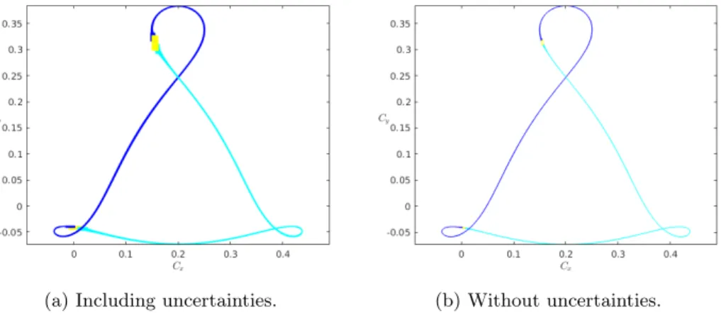
The coupler curve for the design parameters given in (16) is plotted in Fig-ure 2a for ∆θ = 0.001 rad. An uncertainty of ρ = [−0.0001, 0.0001] is added to each design parameter, such that ρ is a vector of uncertainties. For contrast, the coupler curve for the linkage without uncertainties (i.e., the exact design) is plotted in Figure 2b. The appropriate design yields a set of coupler point boxes with larger width than the exact design boxes which demonstrates the greater variation of performance due to the uncertainties. The linkage is classified as a 0π-double-rocker non-Grashof linkage. It has a single circuit containing two different branch assemblies, identified by different colours. Coupler points in the neighbourhood of the toggle position (the transition between branch as-semblies) do not yield unique solutions due to the existence method not being able to guarantee solutions. These regions are simply considered as unknown in terms of coupler point solutions. It is important to note that the size of these regions are proportional to the size and number of uncertainties modelled. The set of intervals provides an outer approximation for the actual coupler curve, i.e., the actual coupler curve is contained inside the union of the set of intervals.
[d] = ([u], [v], [p], [q], [r], [s], [c], [e], [h])T
[d] = ([0.0], [0.0], [0.4], [0.0], [0.24], [0.24], [0.2517], [0.12585], [0.15534])T + ρT (16)
(a) Including uncertainties. (b) Without uncertainties.
Figure 2: The coupler curve corresponding to the design (16).
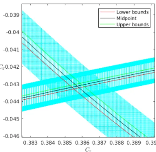
The effect of the uncertainties on the design parameters may be further explored through the coupler curves generated by several exact designs. Here the exact designs are selected as the lower bound, midpoint, and upper bound of the design parameters. The exact coupler curves corresponding to these exact designs are plotted in Figure 3. These coupler curves may also be obtained using Algorithm 2 with the initial [θ] equal to [0]. The solutions are a set of points1 and the curves are approximated by connecting these points. The generated coupler curves may change position with respect to one another, and in fact, due to the non-linearity of the problem, the vertices from the design space are not guaranteed to yield boundaries for the coupler curve. This is an interesting result which demonstrates the difficulties of accounting for uncertainties. It is difficult to know which exact design produces a boundary of the coupler curve of the appropriate design. Even if this design could be determined, it would likely change with the input angle. Thus, determining exactly the coupler curve of an appropriate design proves to be a difficult task.
The method used here allows to bound the worst-case performance of the appropriate design. It is able to compute a tube for the coupler curve that is guaranteed to include all the coupler curves obtained for all specific instances of the design parameters. This simply means that extremal coupler curves (i.e., the ones lying on the boundary of the tube) may be obtained for parameters that are not all on the boundary of the intervals. Interval analysis is guaranteed to
1In this case a point is an interval with minimal width such that it is accurately represented
identify the worst case bounds, whereas alternative methods such as statistical sampling cannot.
Figure 3: A detailed view showing the exact coupler curves corresponding to the lower bound, midpoint, and upper bound of the design parameters from the appropriate design plotted on the coupler curve corresponding to the appropriate design.
To further explore the concept of coupler curves of appropriate designs, appropriate design parameters are selected which correspond to each type of linkage classification, as well as folding linkages. The resulting coupler curves are then presented. For each linkage design, an uncertainty of ρ = [−0.0001, 0.0001] is assumed.
1. A crank-rocker linkage is obtained by selecting the appropriate design parameters as:
[d] = ([0.0], [0.0], [0.4], [0.0], [0.1], [0.4], [0.2517], [0.12585], [0.15534])T + ρT (17) which yields the following values for classification:
[T1] =[0.15130, 0.15211] [T2] =[0.44790, 0.44871] [T3] =[0.15129, 0.15210]
The corresponding coupler curves are given in Figure 4a.
2. A rocker-crank linkage is obtained by selecting the appropriate design parameters as:
[d] = ([0.0], [0.0], [0.4], [0.0], [0.4], [0.1], [0.2517], [0.12585], [0.15534])T + ρT (18)
which yields the following values for classification:
[T1] =[0.15130, 0.15211] [T2] =[−0.15210, −0.15129] [T3] =[−0.44871, −0.44790]
The corresponding coupler curves are given in Figure 4b.
3. A double-crank linkage is obtained by selecting the appropriate design parameters as:
[d] = ([0.0], [0.0], [0.1], [0.0], [0.4], [0.4], [0.2517], [0.12585], [0.15534])T + ρT (19) which yields the following values for classification:
[T1] =[−0.44870, −0.44789] [T2] =[−0.15210, −0.15129] [T3] =[0.15129, 0.15210]
The corresponding coupler curves are given in Figure 4c.
4. A double-rocker linkage is obtained by selecting the appropriate design parameters as:
[d] = ([0.0], [0.0], [0.4], [0.0], [0.4], [0.4], [0.2517], [0.12585], [0.15534])T + ρT (20) which yields the following values for classification:
[T1] =[−0.14869, −0.14789] [T2] =[0.14790, 0.14871] [T3] =[−0.14871, −0.14790] The corresponding coupler curves are given in Figure 4d.
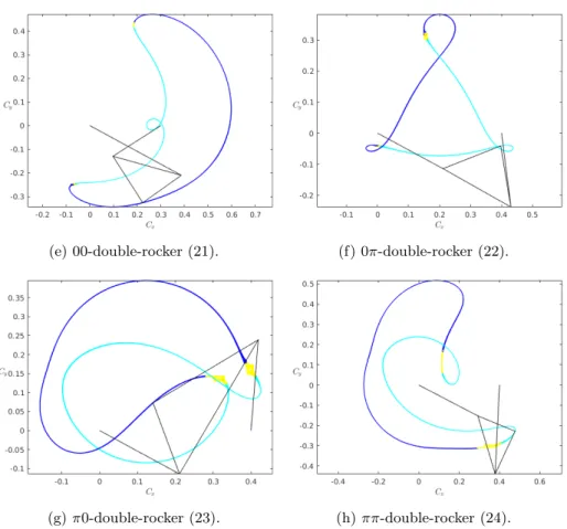
5. A 00-double-rocker linkage is obtained by selecting the appropriate design parameters as:
[d] = ([0.0], [0.0], [0.3], [0.0], [0.44], [0.24], [0.3], [0.12585], [0.15534])T + ρT (21) which yields the following values for classification:
[T1] =[−0.08040, −0.07959] [T2] =[−0.20040, −0.19959] [T3] =[−0.20041, −0.19960] The corresponding coupler curve is given in Figure 4e.
6. A 0π-double-rocker linkage is obtained by selecting the appropriate design parameters as:
[d] = ([0.0], [0.0], [0.4], [0.0], [0.24], [0.24], [0.2517], [0.12585], [0.15534])T + ρT (22)
which yields the following values for classification:
[T1] =[0.17130, 0.17211] [T2] =[0.14790, 0.14871] [T3] =[−0.14871, −0.14790]
The corresponding coupler curve is given in Figure 4f.
7. A π0-double-rocker linkage is obtained by selecting the appropriate design parameters as:
[d] = ([0.0], [0.0], [0.4], [0.0], [0.24], [0.24], [0.41], [0.12585], [0.15534])T + ρT (23) which yields the following values for classification:
[T1] =[0.32960, 0.33041] [T2] =[−0.01040, −0.00959] [T3] =[0.00959, 0.01040]
The corresponding coupler curve is given in Figure 4g.
8. A ππ-double-rocker linkage is obtained by selecting the appropriate design parameters as:
[d] = ([0.0], [0.0], [0.4], [0.0], [0.33], [0.44], [0.3], [0.12585], [0.15534])T + ρT (24) which yields the following values for classification:
[T1] =[−0.07040, −0.06959] [T2] =[0.20960, 0.21041] [T3] =[0.00959, 0.01040]
The corresponding coupler curve is given in Figure 4h.
If the input link is a crank and the linkage is non-folding, then the current existence methods are able to effectively solve for each coupler point interval which corresponds to a given input angle range. If the input link is a rocker, which includes all non-Grashof classifications, then the linkage contains a toggle position which provides a change of branch. The uncertainties present in the linkage make it difficult to guarantee the evaluation of the coupler points near a toggle position using the current existence methods. It may not be possible to identify a unique branch of the linkage near toggle positions. In fact, due to the uncertainties, it is very likely that multiple branches are achievable for certain pairs of input angles and output angles. In addition, the linkage is considered to be singular near toggle positions, and therefore the coupler point becomes extremely sensitive to the input angle. A small input angle will generate a large coupler point box which will cause the existence methods to fail. Note that it is possible to identify the singular region of the coupler curve by adding an
additional constraint that the determinant of the Jacobian of the system is 0. Then the set of input angles and output angles associated with singular regions can be identified.
The sensitivity of the coupler points near toggle positions is witnessed in the coupler curves of Figures 4b, 4d, and 4e to 4h. As the input angle approaches a value which produces a toggle position, the resulting coupler curve interval grows in width. The existence methods are able to accommodate this growth in width to an extent, but eventually the coupler curve interval width exceeds the capabilities of the existence methods. At this point, the remaining portions of the coupler curve can only be approximated and cannot be guaranteed. The input angle may be reduced in width to attempt to obtain additional coupler curve solutions, but limited performance improvements can be achieved by this.
(a) Crank-rocker (17). (b) Rocker-crank (18).
(c) Double-crank (19). (d) Double-rocker (20).
Figure 4: The coupler curves corresponding to appropriate designs with different classifica-tions.
The coupler curve of folding linkages may also be considered. For example: 1. A folding linkage which generates a crank-rocker linkage and a
0π-double-(e) 00-double-rocker (21). (f) 0π-double-rocker (22).
(g) π0-double-rocker (23). (h) ππ-double-rocker (24).
Figure 4: Continued. The coupler curves corresponding to appropriate designs with different classifications.
rocker linkage is obtained by the selecting the appropriate design param-eters as:
[d] = ([0.0], [0.0], [0.4], [0.0], [0.24], [0.34], [0.3], [0.12585], [0.15534])T + ρT (25) which yields the following values for classification:
[T1] =[0.11960, 0.12041] [T2] =[0.11960, 0.12041] [T3] =[−0.00041, 0.00040]
The corresponding coupler curves are given in Figure 5a.
2. A folding linkage which generates a crank-rocker linkage, a rocker-crank linkage, a 0π-double-rocker linkage, and a π0-double-rocker linkage is
ob-tained by the selecting the appropriate design parameters as:
[d] = ([0.0], [0.0], [0.4], [0.0], [0.24], [0.24], [0.4], [0.12585], [0.15534])T + ρT (26) which yields the following values for classification:
[T1] =[0.31960, 0.32041] [T2] =[−0.00040, 0.00041] [T3] =[−0.00041, 0.00040]
The corresponding coupler curves are given in Figure 5b.
(a) Folding linkage (25). (b) Folding linkage (26).
Figure 5: The coupler curves corresponding to appropriate designs with multiple classifications (folding linkages).
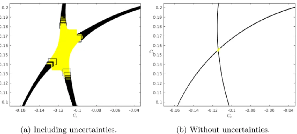
For folding linkages, each coupler point solution has two or more associated classifications. Near the toggle position, the linkage may change from one clas-sification to another, which may be desirable or undesirable given the usage of the linkage. In terms of manufacturing, the manufacturing uncertainties limit the ability to manufacture a linkage to exact specifications. That is not to say that a folding linkage is not possible, as the introduction of other sources of uncertainties (i.e., uncertainties in the joints and flexibility in the links) can in-deed generate a folding linkage. The performance of the folding linkage resulting from uncertainties cannot be determined from exact specifications as the toggle position will no longer be a point, but rather an area. This issue demonstrates the need for linkages described by appropriate designs and analyzed with ap-propriate analysis routines. For example, Figure 6a shows a zoomed-in view of the singular region of the folding linkage (25). For contrast, Figure 6b shows the coupler curve for the same linkage without uncertainties. As the proximity to the singular region increases, the existence methods become unable to de-termine a valid coupler point box which is guaranteed to contain all associated coupler points for some input angle interval and output angle interval. Instead,
(a) Including uncertainties. (b) Without uncertainties.
Figure 6: View of the singular region of the folding linkage (25).
the output angle is repeatedly bisected and simplification routines are applied. The union of the resulting unknown boxes (i.e., the yellow boxes) will still con-tain the coupler curve through the singular region, but the existence of a unique coupler point box cannot be verified. It can be noted that the unknown boxes may better approximate the boundaries of the coupler curve. This is because the union of the coupler point boxes associated with a set of small output an-gles will be smaller than the coupler point box associated with the union of small output angles. At the expense of additional computational time, applying this technique to coupler point solution boxes can allow the boxes to be further reduced in size so that the coupler curve is better approximated.
5. Conclusion
The concept of appropriate design has been presented in this work and meth-ods for the appropriate analysis of the four-bar linkage have been developed. The proposed appropriate analysis techniques provide a new and robust way of accounting for uncertainties present in the geometric parameters of linkages. These techniques rely on interval analysis and are able to provide reliable re-sults. Methods of evaluating the classification and assembly of four-bar linkages described by appropriate designs were introduced, and an appropriate analysis routine for determining the associated coupler curve was proposed. The coupler curves of each classification of linkage, as well as for folding linkages, were pre-sented and the effectiveness of the existence methods near toggle positions was discussed. The performance of the proposed appropriate analysis routine may be further improved by introducing more efficient simplification, existence, and bisection techniques.
This work primarily serves to explore the concept of appropriate design and to introduce relevant appropriate analysis routines which can be applied to study mechanisms. While the four-bar linkage is of primary focus in this work,
the methodology can be extended to study many mechanisms. Many complex-ities (e.g., link flexibility, joint clearance) can be handled by modelling these complexities as uncertainties applied to the kinematic model of the mechanism. The next portion of this work will focus on the appropriate synthesis of the four-bar linkage when provided with a description of a desired response. Ap-propriate synthesis will allow the entire continuous design space to be explored in order to determine the complete set of allowable design solutions which ac-complish a desired response.
References
[1] K.-L. Ting, J. Zhu, D. Watkins, The effects of joint clearance on position and orientation deviation of linkages and manipulators, Mechanism and Machine Theory 35 (3) (2000) 391–401.
[2] G. Chen, H. Wang, Z. Lin, A unified approach to the accuracy analysis of planar parallel manipulators both with input uncertainties and joint clearance, Mechanism and Machine Theory 64 (2013) 1–17.
[3] K.-L. Ting, K.-L. Hsu, Z. Yu, J. Wang, Clearance-induced output position uncertainty of planar linkages with revolute and prismatic joints, Mecha-nism and Machine Theory 111 (2017) 66–75.
[4] J.-P. Merlet, D. Daney, Dimensional synthesis of parallel robots with a guaranteed given accuracy over a specific workspace, in: Proceedings of the 2005 IEEE International Conference on Robotics and Automation, 2005, pp. 942–947.
[5] H. Fang, J.-P. Merlet, Multi-criteria optimal design of parallel manipulators based on interval analysis, Mechanism and Machine Theory 40 (2) (2005) 151–171.
[6] J.-P. Merlet, D. Daney, Smart Devices and Machines for Advanced Man-ufacturing, Springer London, London, 2008, Ch. Appropriate Design of Parallel Manipulators, pp. 1–25.
[7] R. Moore, R. B. Kearfott, M. J. Cloud, Introduction to Interval Analysis, Society for Industrial and Applied Mathematics, 2009.
[8] E. Hansen, G. Walster, Global Optimization Using Interval Analysis: Re-vised And Expanded, Monographs and textbooks in pure and applied math-ematics, CRC Press, 2003.
[9] L. Jaulin, M. Kieffer, O. Didrit, E. Walter, Applied Interval Analysis: With Examples in Parameter and State Estimation, Robust Control and Robotics, Springer London, 2012.
[10] A. Neumaier, Interval Methods for Systems of Equations, Cambridge Mid-dle East Library, Cambridge University Press, 1990.
[11] B. Hayes, A lucid interval, American Scientist 91 (6) (2003) 484–488.
[12] O. Lhomme, Consistency techniques for numeric csps, in: Proceedings of the 13th International Joint Conference on Artifical Intelligence - Volume 1, IJCAI’93, Morgan Kaufmann Publishers Inc., San Francisco, CA, USA, 1993, pp. 232–238.
[13] F. Benhamou, F. Goualard, L. Granvilliers, J. Puget, Revising hull and box consistency, in: Int. Conf. ON Logic Programming, MIT press, 1999, pp. 230–244.
[14] B. Neveu, G. Trombettoni, Adaptive constructive interval disjunction, in: 2013 IEEE 25th International Conference on Tools with Artificial Intelli-gence, 2013, pp. 900–906.
[15] R. Moore, Interval analysis, Prentice-Hall series in automatic computation, Prentice-Hall, 1966.
[16] J.-P. Merlet, Interval analysis for certified numerical solution of problems in robotics, International Journal of Applied Mathematics and Computer Science 19 (3) (2009) 399–412.
[17] R. Kearfott, N. I. Manuel, Intbis, a portable interval newton/bisection package, ACM Trans. on Mathematical Software 16 (2) (1990) 152–157.
[18] J. McCarthy, G. Song Soh, Geometric Design of Linkages, Interdisciplinary Applied Mathematics, Springer, 2010.
[19] T. Chase, J. Mirth, Circuits and branches of single-degree-of-freedom pla-nar linkages, Journal of Mechanical Design - Transactions of the ASME 115 (2) (1993) 223–230.
[20] H. Schr¨ocker, M. Husty, J. McCarthy, Kinematic mapping based assembly mode evaluation of planar four-bar mechanisms, Journal of Mechanical Design 129 (9) (2006) 924–929.