HAL Id: hal-02383496
https://hal.archives-ouvertes.fr/hal-02383496
Submitted on 18 Nov 2020HAL is a multi-disciplinary open access
archive for the deposit and dissemination of sci-entific research documents, whether they are pub-lished or not. The documents may come from teaching and research institutions in France or abroad, or from public or private research centers.
L’archive ouverte pluridisciplinaire HAL, est destinée au dépôt et à la diffusion de documents scientifiques de niveau recherche, publiés ou non, émanant des établissements d’enseignement et de recherche français ou étrangers, des laboratoires publics ou privés.
Where the wild birds go: explaining the differences in
migratory destinations across terrestrial bird species
Marius Somveille, Andrea Manica, Ana S.L. Rodrigues
To cite this version:
Marius Somveille, Andrea Manica, Ana S.L. Rodrigues. Where the wild birds go: explaining the differences in migratory destinations across terrestrial bird species. Ecography, Wiley, 2019, 42 (2), pp.225-236. �10.1111/ecog.03531�. �hal-02383496�
ECOGRAPHY
Ecography
–––––––––––––––––––––––––––––––––––––––– Subject Editor: Morgan Tingley
Editor-in-Chief: Miguel Araújo Accepted 14 June 2018
42: 225–236, 2019
doi: 10.1111/ecog.03531
doi: 10.1111/ecog.03531 42 225–236
Given their large movement capacities, migratory birds have in principle a wide range of possible geographical locations for their breeding and non-breeding destinations, yet each species migrates between consistent breeding and non-breeding ranges. In this study, we use a macroecological approach to search for the general factors explaining the location of the seasonal ranges of migratory bird species across the globe. We develop a null model to test the hypotheses that access to resources, geographical distance, tracking of temperature, and habitat conditions (separately as well as considered together) have a major influence in the location of species’ migratory destinations, once each species’ geographical constraints are taken into account. Our results provide evidence for a trade-off between costs associated with distance travelled and gains in terms of better access to resources. We also provide strong support to the hypotheses that all factors tested, with the exception of habitat, have a strong and additive effect on the global geography of bird migration. Indeed, our results indicate that species’ contemporary migratory destinations (i.e. the combination of their breeding and non-breeding ranges) are such that they allow species to track a temperature regime throughout the year, to escape local competition and reach areas with better access to resources, and to minimise the spatial distance travelled, within the limitations imposed by the geographical location of each species. Our study thus sheds light on the mechanisms underpinning bird migration and provides a strong basis for predicting how migratory species will respond to future change.
Keywords: bird migration, seasonality, migration destinations
Introduction
With their capacity to travel great distances, migratory birds have in theory a wide range of possible breeding and non-breeding destinations, yet each species has consistent seasonal geographical ranges. Given that migration is a costly behaviour, both in terms of energy and mortality (Sillett and Holmes 2002, Wikelski et al. 2003, Newton 2006, Klaassen et al. 2014, Lok et al. 2015), there must be a net benefit
Where the wild birds go: explaining the differences in
migratory destinations across terrestrial bird species
Marius Somveille, Andrea Manica and Ana S. L. RodriguesM. Somveille (http://orcid.org/0000-0002-6868-5080) ([email protected]), The Edward Grey Inst., Dept of Zoology, Univ. of Oxford, Oxford, UK. – A. Manica and MS, Dept of Zoology, Univ. of Cambridge, Cambridge, UK. – A. S. L. Rodrigues and MS, Centre d’Ecologie Fonctionnelle et Evolutive CEFE UMR 5175, CNRS – Univ. de Montpellier – Univ. Paul-Valéry Montpellier – EPHE, Montpellier, France.
in moving between specific seasonal ranges for each spe-cies’ migratory behaviour to persist (Lack 1968). Yet there does not seem to be a simple common rule across species explaining the geographical location of these seasonal ranges. For example, whereas some species travel relatively short distances (e.g. Henslow’s sparrow Ammodramus henslowii, within eastern North America), others make extensive jour-neys across continents and seas (e.g. veery Catharus fuscescens, between North and South America). And while some species use a consistent habitat type throughout the year (e.g. pied wheatear Oenanthe pleschanka, favouring open areas), oth-ers switch between different habitats types (e.g. pechora pipit
Anthus gustavi, breeding in the Siberian bushy tundra and
wintering in tropical southeast Asian forests).
Most studies investigating what drives the geographical location of breeding and/or non-breeding destinations focus on particular species, proposing idiosyncratic explanations based on their ecology or physiology. For example, several studies have investigated how migratory destinations can satisfy the particular ecological needs of the studied species, such as by investigating how it affects the energy balance of individuals given their physiological tolerance (West 1958, Cox 1961), but those findings are not easily generalizable to other species. Other studies have proposed mechanisms driv-ing variation in the diversity of migratory birds across broad geographical space (Newton 1995, Hurlbert and Haskell 2003, Dalby et al. 2014, Somveille et al. 2015), but without explaining why different species do different things. Taken together, however, these studies have highlighted several factors that may affect the geographical location of migratory species’ breeding and non-breeding grounds.
First, the seasonality in resources appears as a significant explanatory variable in multi-species studies searching for general rules to explain spatial patterns of migratory bird diversity (Dalby et al. 2014, Somveille et al. 2015). Indeed, migratory birds tend to breed in regions with a surplus of resources during the breeding season, and then redistribute to the nearest suitable non-breeding grounds (Somveille et al. 2015). Regions with strong seasonality may be particularly suitable to migrants because the resource availability dur-ing the least productive season (typically the winter) limits the number of (and thus competition with) resident species (Herrera 1978, Hurlbert and Haskell 2003, Dalby et al. 2014, Somveille et al. 2015). Hence, even though these studies did not attempt to explain the differences in migratory destina-tions across species, their results suggest that the geographical location of species’ breeding and non-breeding grounds may be driven by benefits in terms of access to resources that are not competed for by resident species.
Second, previous studies showed that the cost of migra-tion increases with distance travelled, as energy expendi-ture (Wikelski et al. 2003) and mortality risks (Lok et al. 2015) increases. Hence, minimising the distance travelled should be a selective advantage, as the extra energy used during migration and the increased mortality are expected to reduce the fitness of the individuals, unless it results in a
higher benefit (Lack 1968), for example in terms of access to available resources and/or better tracking of environmental conditions.
Third, a number of studies have demonstrated that a species’ ecological niche (the suite of environmental con-ditions within which it can maintain viable populations; Hutchinson 1957) constitutes an important constraint to its distribution (Tingley et al. 2009, Pigot et al. 2010, Chen et al. 2011). Accordingly, species may migrate in order to track favourable environmental conditions throughout the year. Whilst birds (like other endotherms) can regulate their internal body temperature even when ambient tempera-ture is outside their thermal optimum, this has an energetic cost (Kendeigh 1969, Porter and Kearney 2009). Seasonal variation in climate, and particularly temperature, can thus impose a non-negligible cost to resident species, resulting in an important widening of their overall climatic niche (Janzen 1967). Previous studies have yielded conflicting results in this regard, suggesting it is not a universal mechanism to explain migration destinations. Indeed, early studies focusing on New World migratory birds have found that some species follow their climatic niche throughout the year (niche fol-lowers) while others switch niche seasonally (niche switchers; Martínez-Meyer et al. 2004, Nakazawa et al. 2004). More recently, Boucher-Lalonde et al. (2014) analysed data on migratory birds in the Americas across families and concluded that migration does not result in tracking of the thermal niche, but Gomez et al. (2016) found that migratory New World warblers (Parulidae) track temperature conditions to a greater extent than residents. In addition, Laube et al. (2015) found that migratory Old World Sylvia warblers did not compensate for the cost of longer journeys by tracking climatic conditions more closely. The importance of climate tracking in explaining the differences in breeding and non-breeding destinations across migratory birds is therefore not fully understood, and these mixed results indicate that other factors must also be at play.
In addition to climate, another characteristic of the envi-ronment that has been shown to affect the distribution of bird species, thus potentially constraining the geographical loca-tion of breeding and non-breeding grounds, is habitat type (Barnagaud et al. 2012). Bilcke (1984) hypothesised that the reason why long-distance migrants breeding in Europe prefer more open habitats than those breeding in North America is due to a difference in wintering habitats, with the underlying assumption that migratory bird species ‘use the same kinds of habitats in their wintering and breeding grounds’ (Helle and Fuller 1988). However, Dalby et al. (2014) found that habitat explained only little of the global seasonal distribu-tion of waterfowl species richness, compared to productivity and temperature. However, to our knowledge, no study has formally tested if habitat requirements constrain the location of the breeding and non-breeding grounds of migrant birds across many species and wide spatial scales.
An additional factor that likely affects species’ migratory destinations is the constraints imposed by their geographical
location. Indeed, as breeding and non-breeding grounds are necessarily linked together, the location of each one affects the options a species has for the other season. Hence, for exam-ple, migration options are not the same for species breed-ing in Europe vs Siberia or winterbreed-ing in western vs eastern sub-Saharan Africa. Accordingly, Somveille et al. (2015) found that the diversity of non-breeding migrants is related to how connected the area is to regions that are particularly suitable as breeding grounds. However, to our knowledge, no previous study has explicitly incorporated geographical con-straints in analyses to understand the differences in migratory destinations across species.
These drivers and constraints are not mutually exclusive, and may affect each species differently. In this study, we use data on the breeding and non-breeding geographical ranges of terrestrial bird species at the global scale to search for a common set of rules explaining why each migratory species migrates between its respective breeding and non-breeding grounds. We assume that current ranges are the result of evo-lutionary processes and must, therefore, be adaptive, but our aim is not to explain how migration itself evolved or how each species’ seasonal ranges ended up in their contemporary locations. Instead, we ask whether the geographic location of current ranges is influenced by a set of costs and benefits, as a means to test hypotheses about the ecological drivers and constraints to bird migration.
We start by measuring, for each species in our dataset, and given their breeding and non-breeding ranges, four vari-ables: the year-round benefits in terms of accessing resources; the geographical distance separating the breeding and non-breeding grounds; the inter-seasonal distance in thermal con-ditions; and the inter-seasonal distance in habitat conditions. This allowed us to investigate whether the geographical loca-tion of species’ migratory destinaloca-tions is affected by trade-offs between access to resources, migration distance and tracking environmental conditions (temperature and habitat). We then integrated the effect of the species-specific geographi-cal constraints by developing a null model that controls for the migration options available to each species. We simulated for each migratory species a set of possible alternative breed-ing and non-breedbreed-ing distributions (similar in size and shape to the observed ranges), from which we derived alternative (simulated) migration options. By comparing the observed migration destinations with the alternative options in terms of access to resources, migration distance, tracking of temper-ature and tracking of habitat, we tested the hypotheses that these costs-benefits variables, alone and/or in combination, drive the geography of species’ migrations.
Material and methods
Species distribution data
All analyses were based on a dataset representing the global distribution of 9783 land bird species, mapped by BirdLife International and NatureServe (2012) as polygons
representing species’ broad ranges. Range maps were con-verted into presences–absences on a grid of equal-area,
equal-shape hexagons (7352 hexagons, ~23 322 km2 each;
Sahr et al. 2003, Somveille et al. 2013) covering the world land masses. This dataset includes only species occurring predominantly on land (for which > 50% of either their breeding or their non-breeding range overlap land).
As in previous studies (Somveille et al. 2013, 2015), we defined migratory species as those whose breeding and non-breeding distributions did not completely overlap, totalling 1403 species. For many of these species, there are parts of their range where they are present in both the breeding and non-breeding seasons, but our dataset does not allow us to distinguish whether the populations in these areas are resi-dent (i.e. the same individuals are present year-round) or migratory (i.e. different individuals are present in different seasons). In order to focus our analyses on populations that are very likely to be migratory, we considered only the 621 migrant species that have less than 20% overlap between their breeding and non-breeding ranges. This was a pragmatic threshold: a compromise between higher certainty that our analysis focus on fully migratory species and keeping a larger number of species in the dataset.
We treated the Western Hemisphere (< 30°W) and the Eastern Hemisphere (> 30°W) separately since no migra-tory bird species has its entire breeding range on a different hemisphere from its entire non-breeding range. Some wide-spread species have breeding and nonbreeding ranges across both hemispheres (22 species). For those, we have treated the population of each hemisphere separately, effectively treating them as two different species. Overall, we analysed 643 populations, which are for simplicity referred to as ‘species’ throughout the text.
We defined seasons based on the two extremes of seasonality in the year across most of the world, by concen-trating on two time periods: from May to August, and from November to February, corresponding respectively to sum-mer and winter in the Northern Hemisphere and to win-ter and summer in the Southern Hemisphere. Our original dataset indicates which part of each species’ range is breeding and which is non-breeding, but not whether species breed during the northern summer or during the northern winter. We assumed that all species whose entire breeding range falls within latitudes superior to 30°N breed during the north-ern summer and occupy their non-breeding range during the northern winter, and vice-versa for species at latitudes superior to 30°S. For the remaining species, we obtained information on their breeding season from the literature (in particular from The handbook of the birds of the world; Del Hoyo et al. 1992–2011).
Drivers and constraints of migration Measuring access to resources
We assumed that the normalized difference vegetation index (NDVI; a remote sensing measure of greenness) is a general indicator of the resources (food, nest sites, roosting sites)
available to bird species. We obtained average monthly esti-mates of NDVI from NASA’s Earth Observatory (resolution 0.1°; averages obtained from 2006 to 2014; NASA’s Earth Observatory 2014). NDVI values (multiplied by 100) ranged between −10 and 90 (the higher the value, the greener the land). Barren areas of rock, sand or snow (NDVI < 0), and areas above the Arctic Circle during the northern win-ter (no data) were coded as 1 for analytical purposes (as in Somveille et al. 2015). NDVI values for each hexagon were obtained by averaging the values across the pixels within each hexagon. We then obtained seasonal estimates by aver-aging values across May to August and across November to February.
As in previous studies (Herrera 1978, Hurlbert and Haskell 2003, Dalby et al. 2014, Somveille et al. 2015) we assumed that the resources available to migrant species are related to the surplus in NDVI, i.e. the difference between NDVI in the season when the migrant birds are present and the season when they are absent. This is in turn based on the assumption that resident species take the resources com-mon to both seasons, an assumption supported by a strong positive relationship between the richness in resident species (obtained as counts per hexagon of resident species, using the geographical ranges of 7820 resident species in Birdlife International and NatureServe 2012) and the NDVI per
hexagon in the least productive season (n = 6649; regression
model: slope = 4.07, t = 127.5, p < 0.0001, R2= 0.71).
For each species, and for each seasonal range, we measured for each hexagon within the range the difference between the NDVI in the season when the species in present and the NDVI in the season when the species is absent. A positive value means that a seasonal resource surplus is available to the species in the hexagon (the higher this value, the more abundant those resources); a negative value means a deficit. We averaged the values across all hexagons within each of the seasonal (breeding or non-breeding) ranges of the species to obtain a value of NDVI surplus per season. We then summed these two values and took the opposite of that sum to obtain an overall measure of ‘resource scarcity’ per species through-out the year. This is negative if the species’ combination of breeding and non-breeding ranges brings it a net surplus in NDVI over the year, and positive if the species experiences a net deficit. We formulated it this way so resource scarcity is a measure of the costs of migration, like the other variables we considered.
Measuring inter-seasonal geographical distance
We assumed that the costs associated with the migration movement itself increased linearly with the geographical dis-tance between breeding and non-breeding areas. For each species, we measured this cost as the great-circle distance between the centroids of the breeding and non-breeding ranges.
Measuring inter-seasonal thermal distance
To quantify the temperature conditions during one season, we combined two variables: average seasonal temperature, affecting the average thermo-regulation cost experienced by
a species across the season; and minimum seasonal tempera-ture, representing the extreme variation of temperature likely to affect the thermo-regulation cost of the species during the season.
We obtained monthly minimum and average tempera-ture data for 1970 to 2000 from WorldClim 2.0 (resolution 2.5 minutes; Fick and Hijmans 2017). For each hexagon, we obtained seasonal values of average temperature by taking the mean of the average temperature values across the four months of each of the two opposite seasons (May to August and November to February). Similarly, we obtained seasonal values of minimum temperature for each hexagon by taking the minimum of the minimum temperature values across the four months of each of the two opposite seasons (May to August and November to February). These two variables were normalised and together defined a two-dimensional thermal space (with axes corresponding to a normalized average tem-perature extent of [–3.4, 1.6] and a normalized minimum temperature extent of [–3.3, 1.4]) on which all measures of thermal distance were computed.
For each species, in each season (i.e. breeding or non-breeding), we characterised the seasonal temperature con-ditions in two steps. First, we projected all occurrences (i.e. hexagons) for the corresponding season into the above-mentioned general thermal space, thus obtaining a cloud of points. Second, we converted this cloud of points into a two-dimensional seasonal density kernel on a 20 × 20 grid super-imposed onto the thermal space, representing a probability distribution landscape (using the ‘kde2d’ function in R with a bandwidth of 1). The choice of a 20 × 20 grid is arbitrary: a compromise between ensuring sufficient detail whilst avoid-ing excessive computavoid-ing times. We kept only the top 99% of the density kernel (i.e. pixels with the highest probability values and whose sum correspond to 99% of the density of the probability surface) and set the rest of the pixels to 0.
For each species, we then measured the inter-seasonal thermal distance by computing the Earth Mover’s Distance (EMD) between the breeding and non-breeding probabil-ity distribution landscapes in the general temperature space. The EMD is an algorithm that was originally developed for image comparison (Rubner et al. 2000) and has been recently adapted to quantify similarity between spatial utilization distributions (Kranstauber et al. 2016). It provides a dis-tance measure by calculating the effort it takes to shape one probability distribution landscape into another. The imple-mentation in the R package ‘move’, originally designed for comparing probability distributions in geographical space, can be directly used in a two-dimensional climate space. The EMD has important advantages over other standard niche dis-tance measures, such as overlap (as in Boucher-Lalonde et al. 2014) or distance between centroids. Indeed, it can provide a reliable distance measure between a pair of two-dimensional probability distributions even if the overlap between them is 0 or near 0, is less sensitive than other measures to variation in area of the two distributions (Kranstauber et al. 2016), and takes into account variations in density within each probabil-ity distribution.
Measuring inter-seasonal habitat distance
As a measure of the habitat type in which each species occurs in each season, we quantified the degree of closeness of the habitat across each seasonal geographical distribution. To do so, we used the land cover classification in the global MODIS land cover dataset (0.5° resolution, Channan et al. 2014). Following a methodology similar to Somveille et al. (2016), we coded: forests pixels as closed habitat with a value of 1; savannas, grasslands, wetlands, croplands, snow and ice, and barren or sparsely vegetated pixels as open habitat with a value of 0; and shrublands, woody savannas, and cropland/natural vegetation mosaic pixels as partially closed habitat with a value of 0.5. We then averaged the values of all pixels within each hexagon to obtain a value per hexagon. And then, for each species in each season, we quantified the average habitat value across all hexagons in the corresponding seasonal range. Finally, the inter-seasonal habitat distance was computed per species as the absolute difference between the breeding habitat value and the non-breeding habitat value.
Investigating trade-offs between variables
We tested the hypothesis that species migrate further to bet-ter track environmental conditions (i.e. tracking a tempera-ture regime or being constrained by habitat type) by testing for significant negative relationships between geographical distance and thermal and habitat distances (by computing an ordinary least squares model, allowing for a quadratic
term, and reporting the goodness-of-fit, R2). In a similar way,
we tested the hypothesis that species migrate further to gain better access to resources by testing for a negative relation-ship between geographical distance and resource scarcity. Furthermore, we tested whether there is a trade-off between thermal distance, habitat distance and resource scarcity by investigating the relationship between these variables. Finally, we investigated the relationship among tracking environmen-tal conditions, better access to resources and geographical distance through a three-dimensional plot.
Null model: comparing species’ observed migrations with simulated alternatives
Simulating alternative migrations
For each species, we obtained a set of simulated alternative breeding and non-breeding ranges, with similar characteris-tics (size and shape) to the real ranges but located randomly.
We started by characterising each of the species’ two sea-sonal ranges (breeding and non-breeding) in terms of size and shape. Typically, seasonal ranges are composed of a single contiguous block of hexagons, but sometimes they consist of separate blocks. For each range, we counted the number of blocks and the size of each (i.e. number of hexagons). We described the shape of each block as the number of occupied hexagons at 30° intervals along a clock-wise 360° rotation (starting from the north bearing) departing from the centroid of the block, thus obtaining a density function of presence (Supplementary material Appendix 1 Fig. A1).
To simulate a given block of hexagons, we started by selecting one hexagon at random in the relevant land mass (i.e. Western Hemisphere or Eastern Hemisphere), and then used the density function of presence (Supplementary material Appendix 1 Fig. A1B) to associate a probability to each of the hexagon’s neighbours based on the bearings of the rhumb lines between hexagon centroids (Supplementary material Appendix 1 Fig. A1A, C). In each step, we selected at random 25% of these neighbours (rounded to the larger integer), weighted by the corresponding probabilities. We then repeated this procedure, selecting every time among the neighbours of all the previously occupied hexagons (Supplementary material Appendix 1 Fig. A1D) until reach-ing the size of the observed block (i.e. same number of hexa-gons). At each of these steps, all the bearings to the neighbours were calculated from the first central hexagon. This generated a simulated contiguous block of hexagons that broadly repli-cates the shape of a real block while respecting the constraints imposed by the shape of landmasses.
For disjoint seasonal ranges (i.e. composed of multiple contiguous blocks of hexagons), we simulated the blocks in order of size, starting from the largest. We placed the second largest block such that its centroid was at a similar distance from the largest block as in the real range. We then placed any subsequent block such that the sum of the distance between its centroid and each of the two largest simulated blocks was approximately the same as the sum of distances observed in the real range. In order to allow a range of possibilities in the placement of this block’s central hexagon, we obtained its position by randomly selecting one of the 20 hexagons for which the sum of the distances to the centroids of the two largest contiguous blocks was the closest to the observed value. This ensures that the simulated set of blocks has rela-tive positions that are comparable to those in the real range, while respecting the geographic constraints of the region.
For each migratory species, we simulated 100 alternative breeding ranges and 100 alternative non-breeding ranges. We obtained 200 simulated alternative migrations by pair-ing a species’ true range in a given season with an alternative simulated range for the opposite season.
Performance of the observed migration in relation to the simulated alternatives
For each species, and for each simulated alternative migra-tions, we computed: resource scarcity; inter-seasonal geo-graphical distance; inter-seasonal thermal distance; and inter-seasonal habitat distance. For each of these variables, we then ranked the value for the observed migration among the 200 migration alternatives (Supplementary material Appendix 1 Fig. A2C). Specifically, we counted how many among the alternatives have lower values than the observed migration and divided by 200, thus obtaining for each spe-cies a scaled rank value between 0 (the observed migration is better than all alternatives) and 1 (the observed migration is worse than all alternatives).
For any given variable, we test the hypothesis that it drives the location of species’ migratory destinations by plotting
the frequency distribution of scaled ranks and testing (using one-sided Kolmogorov–Smirnov tests) if this frequency is left skewed towards lower ranks. Indeed, if that is what would be expected if, across species, the observed migrations tend to have lower values (i.e. lower costs for the variable) compared to the alternative migration options available to each species (given its geographical constraints). In contrast, if the loca-tion of migraloca-tion destinaloca-tions is not affected by the variable in question, we would expect a uniform distribution of the frequencies of scaled ranks.
To test for the combined effects of multiple variables, we extended this approach to combinations of two, three or four variables. To obtain scaled ranks for combinations of vari-ables, we first normalized each of the variables across all 201 values (200 simulated migrations plus the observed one), and then summed the values for the relevant combinations of variables (e.g. normalized geographical distance plus normal-ized thermal distance; Supplementary material Appendix 1 Fig. A2C). As above, we obtained for each species a scaled rank value between 0 and 1, first by counting how many alter-natives have lower summed values than the observed migra-tion (Supplementary material Appendix 1 Fig. A2C, D) and then by dividing this rank by 200. We investigated if there is (across species) a signal that the combined variables drive the migration destinations of species, by plotting the frequency distributions of scaled ranks for combinations of variables, and tested whether these distributions are skewed towards lower ranks using one-sided Kolmogorov–Smirnov tests.
This approach tests the hypotheses that the location of contemporary migratory ranges is driven by the four vari-ables tested (in isolation or in combination), without asking how specific ranges ended up where they are in evolutionary time. As such, it implicitly assumes that current ranges are close to equilibrium with current environmental conditions, i.e. that species have had enough time to optimise the loca-tion of their migratory destinaloca-tions. This assumploca-tion seems reasonable for most species given the high mobile capacity of birds, and evidence that some species are changing migra-tory routes in response to on-going environmental change (Berthold et al. 1992, Sutherland 1998, Gilbert et al. 2016).
Mapping the performance of observed migrations in relation to simulated alternatives
As detailed below, we found that the best combination of variables (the one that produced the most left skewed distri-bution) was the combination of tracking temperature condi-tions, access to resources and geographical distance separating migratory destinations. For each hexagon of the global spatial grid, we calculated the average scaled rank for this combina-tion of variables, calculated among all species present in the hexagon in either their breeding or their non-breeding ranges. We used these values to map global patterns in the apparent performance of observed migrations, presenting separately results for breeding and non-breeding migrants. Low values correspond to regions dominated by species whose observed migrations are consistent with the hypothesis that the three
variables (tracking temperature conditions, access to resources and geographical distance separating migratory destinations) together drive the location of migratory ranges. In contrast, regions with high values are dominated by species whose observed migrations appear to perform poorly in relation to the migration destinations available to them, and thus for which our modelling framework does not adequately explain migration destinations.
We complemented these with global maps showing the geographical distance travelled by each species (plotted as curves representing the great circle distance between the centroids of breeding and non-breeding ranges), presenting separately species that appear to perform well (scaled rank < 0.1), moderately well (0.1 ≤ scaled rank < 0.5) and poorly (scaled rank ≥ 0.5) under our modelling framework.
Finally, we analysed the geographic locations of the simulated migration destinations that (for any given species) appeared to perform better than the observed ones. These results are presented in the Supplementary material Appendix 1–3.
Code availability
The codes used to run the analyses and produce the figures presented in this paper are available in the appen-dix (Supplementary material Appenappen-dix 2) as well as at <
https://github.com/msomveille/bird-migration-diversity-analysis.git >.
Results
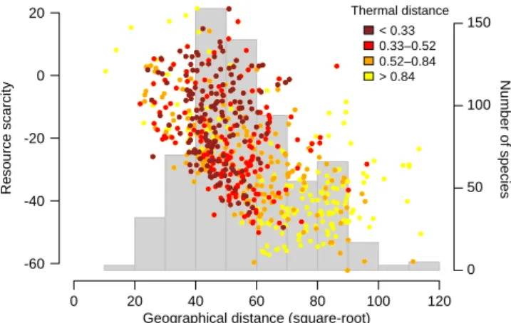
For 91% of migratory species, migration seems to result in a net benefit in access to available resources (i.e. nega-tive values in our measure of resource scarcity; Fig. 1). The magnitude of this benefit increases with the distance trav-elled between the breeding and non-breeding grounds as indicated by the strong negative relationship (correlation
coefficient ρ = –0.54) between geographical distance and
resource scarcity, supporting the hypothesis that species travel further to gain better access to available resources (i.e. lower resource scarcity values; Fig. 1). The species that bet-ter track temperature conditions concentrate at inbet-termediate points along this trade-off (Fig. 1 and Supplementary mate-rial Appendix 1 Fig. A3A), travelling intermediate distances for relatively moderate gains in access to resources, these intermediate distances being also the norm across all migra-tory species (histogram in Fig. 1). This result contrasts with what would have been expected if species travelled longer dis-tances to better track temperature conditions. We also found a slightly negative relationship between tracking temperature conditions and better access to resources (Supplementary material Appendix 1 Fig. A3B), indicating that species whose migration allows them to have high gains in access to resources tend to experience substantially different tempera-ture conditions between their breeding and non-breeding seasons (and also travel longer distances; Fig. 1). We did not
find, however, relationships between habitat distance and the other variables, apart for a slightly positive but not signifi-cant trend with geographical distance (Supplementary mate-rial Appendix 1 Fig. A3C). In other words, habitat tracking does not seem to affect the distance separating the breeding and non-breeding grounds of migratory species, the degree to which they track temperature conditions, or the access to resources.
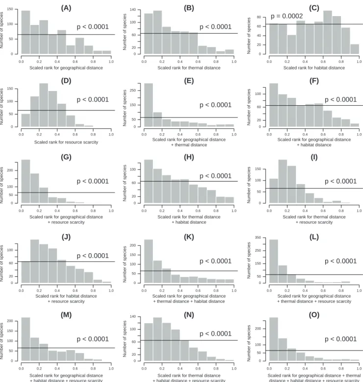
Overall, observed migrations tend to perform better than most of the simulated alternatives for geographical distance, thermal distance and resource scarcity, either considered separately or in combination (Fig. 2). Indeed, we found in all cases involving these variables a frequency distribution of the scaled ranks of the observed migration among alterna-tives significantly skewed towards low values (Fig. 2; for all two-sample Kolmorov–Smirnov tests p-values < 0.0001). This pattern became more pronounced when several vari-ables where combined, suggesting additive effects of multiple variables (Fig. 2). In fact, all frequency distributions of ranks for combinations of these three variables were significantly skewed towards low values when compared to frequency dis-tributions of ranks for subsets of variables (i.e. single vari-ables, or combinations two variables when compared to the three variables together; Supplementary material Appendix 1 Table A1), which indicates that, when considered, each of these variables (geographical distance, thermal distance and resource scarcity) improved the ranks of observed migrations across species. Habitat distance, however, did not significantly improve the ranks of species’ migrations when compared to alternative options (i.e. when habitat distance was included, it did not result in a frequency distribution of ranks that was
more skewed towards low values) for any of the combinations of variables (Fig. 2 and Supplementary material Appendix 1 Table A1). The best (most parsimonious) combination of variables was therefore the one will all variables except habitat distance. This combination was then used for generating the maps (Fig. 3 and 4) and it is the focus of our discussion.
We found strong spatial patterns in the extent to which species’ migratory ranges seem to perform under our model-ling framework, i.e. in terms of the combination of geograph-ical distance, thermal distance and resource scarcity, given geographical constraints (Fig. 3 and 4). Species that appear to perform well are mainly intra-continental migrants, thus with relatively short migration distances (Fig. 3A), whereas species with moderate performances are often inter-continental migrants with longer migration distances (Fig. 3B). The species with the worst performances tend to migrate very long distances between breeding grounds at high northern lati-tudes and non-breeding grounds in the southern hemisphere (Fig. 3A, B and 4C).
Discussion
Our results provide support to the hypothesis that migra-tion allows species to track a temperature regime through-out the year (Fig. 2). This appears to somewhat contradict the results obtained previously by Boucher-Lalonde et al. (2014) and by Laube et al. (2015). However, their analy-ses applied a different method for studying niche track-ing in migratory birds. Indeed, these authors quantified the overlap between environmental envelopes representing the breeding and non-breeding niches of migrants; having found little overlap (no better than the null expectation from randomisation models), they concluded that migra-tion does not result in niche-tracking. But their measure considers as equivalent all species whose seasonal niches do not overlap at all, even if those species differ substantially in the distance between their niches. They also only com-pared observed migrations to the alternative scenario of no migration at all and to a randomisation of migratory species’ ranges. In contrast, we use in this study a more general null model, comparing the observed migrations to alternative simulated migrations. Our result that the observed thermal distance across seasons (computed using the Earth Mover’s Distance; Kranstauber et al. 2016) appears to perform well when compared the alternative options (Fig. 2B) thus provide evidence for tracking of temperature conditions via migration. Whereas our approach explicitly takes into account seasonal variation in temperature as well as spatial variation in temperature across species’ ranges, it does not fully consider within-season temporal variation in tempera-ture, other than by taking into account the minimum tem-perature within season in addition to the average. However, Quintero and Wiens (2013) found that climatic variation between sites across a species’ range strongly correlates with temporal niche breadths, which indicate that it might not be necessary to use both.
0 50 100 150
0 20 40 60 80 100 120
Geographical distance (square-root)
Resource scarcity -60 -40 -20 0 20 Number of specie s Thermal distance < 0.33 0.33–0.52 0.52–0.84 > 0.84
Figure 1. Relationships between the geographical distance separat-ing the breedseparat-ing and non-breedseparat-ing ranges, the year-round availabil-ity of surplus primary productivavailabil-ity and temperature difference between the breeding and non-breeding seasons (thermal distance) across migratory species. Resource scarcity measures the opposite of the year-round availability of surplus primary productivity, and was used for convenience throughout the analyses. Each point repre-sents a species, positioned in terms of its values for inter-seasonal geographical distance and resource scarcity. The relationship is coloured according to inter-seasonal thermal distance to obtain a three-dimensional plot. The background histogram indicates the number of species for each class of geographical distance.
Tracking of temperature conditions was not perfect (thermal distances were never zero) and several species appear not to track a temperature regime at all (Fig. 2B). This observation is in line with previous studies that found that some migratory species follow their niche throughout the year while others switch niche seasonally (Martínez-Meyer et al. 2004, Nakazawa et al. 2004), and suggests that other factors contribute to determining
migration destinations of birds. In addition, the degree to which migratory species track temperature conditions increased with increasing the geographical distance travelled (Fig. 1 and Supplementary material Appendix 1 Fig. A3A), in contrast with previous findings (Laube et al. 2015).
Our results also support the hypothesis that migration allows birds to escape local competition and reach areas
0.0 0.2 0.4 0.6 0.8 1.0 0 50 100 150 Number of specie s
Scaled rank for geographical distance
(A) p < 0.0001 0.0 0.2 0.4 0.6 0.8 1.0 0 20 60 100 140 Number of specie s
Scaled rank for thermal distance
(B) p < 0.0001 0.0 0.2 0.4 0.6 0.8 1.0 0 20 40 60 80 Number of specie s
Scaled rank for habitat distance
(C) p = 0.0002 0.0 0.2 0.4 0.6 0.8 1.0 0 50 100 150 Number of specie s
Scaled rank for resource scarcity
(D) p < 0.0001 0.0 0.2 0.4 0.6 0.8 1.0 0 50 150 250 Number of specie s
Scaled rank for geographical distance + thermal distance (E) p < 0.0001 0.0 0.2 0.4 0.6 0.8 1.0 0 20 60 100 Number of specie s
Scaled rank for geographical distance + habitat distance (F) p < 0.0001 0.0 0.2 0.4 0.6 0.8 1.0 0 50 100 200 Number of specie s
Scaled rank for geographical distance + resource scarcity (G) p < 0.0001 0.0 0.2 0.4 0.6 0.8 1.0 0 20 60 100 Number of specie s
Scaled rank for thermal distance + habitat distance (H) p < 0.0001 0.0 0.2 0.4 0.6 0.8 1.0 0 50 100 150 Number of specie s
Scaled rank for thermal distance + resource scarcity (I) p < 0.0001 0.0 0.2 0.4 0.6 0.8 1.0 0 20 60 100 Number of specie s
Scaled rank for habitat distance + resource scarcity (J) p < 0.0001 0.0 0.2 0.4 0.6 0.8 1.0 0 50 100 150 200 Number of specie s
Scaled rank for geographical distance + thermal distance + habitat distance
(K) p < 0.0001 0.0 0.2 0.4 0.6 0.8 1.0 0 50 150 250 350 Number of specie s
Scaled rank for geographical distance + thermal distance + resource scarcity
(L) p < 0.0001 0.0 0.2 0.4 0.6 0.8 1.0 0 50 100 150 200 Number of specie s
Scaled rank for geographical distance + habitat distance + resource scarcity
(M) p < 0.0001 0.0 0.2 0.4 0.6 0.8 1.0 0 20 60 100 140 Number of specie s
Scaled rank for thermal distance + habitat distance + resource scarcity
(N) p < 0.0001 0.0 0.2 0.4 0.6 0.8 1.0 0 50 100 200 Number of specie s
Scaled rank for geographical distance + thermal distance + habitat distance + resource scarcity
(O)
p < 0.0001
Figure 2. Frequency distributions of the scaled ranks of each species’ observed migration among alternative simulated options. The black horizontal lines indicate the uniform expectation under a random null model. The p-values in each histogram correspond to the Kolmogorov– Smirnov test of whether the observed distribution is left-skewed compared to the uniform distribution.
where they have better access to resources (Lack 1954, 1968, Fretwell 1980). Indeed, we found that for the large majority of species (91%), migration allows them to experience a net surplus in NDVI over the year (negative resource scarcity; Fig. 1). Accordingly, a previous study found that regions with a higher seasonal surplus in resources have higher richness in breeding migrants (Somveille et al. 2015). We also found that, overall, species tend to trade-off between the benefits in terms of better access to resources and the costs of travel-ling (Fig. 1). The species reaping the higher benefits in terms of accessing a surplus of resources tend to travel the longest distances (Fig. 1), and often experience substantially different temperature conditions between the two seasons (Fig. 1). Most species, however, tend to be relatively good at track-ing thermal conditions closely throughout the year, dotrack-ing so by travelling intermediate geographical distances and having moderate gains in terms of access to resources (Fig. 1).
Our results provide no evidence that habitat constrains migratory destinations, at least as measured in terms of habitat openness related to tree cover. Indeed, habitat distance varies independently of other variables, providing no evidence of a trade-off between them (Supplementary material Appendix 1 Fig. A3). Moreover, it did not improve the results for the
null model whatever the combination of variables (Fig. 2 and Supplementary material Appendix 1 Table A1). This suggests that the constraints imposed by species’ ecologies and adap-tations to habitat openness do not play a major role in the selection of their migratory destinations. It is however pos-sible that habitat selection plays a role at a finer spatial scale, within broad species’ seasonal geographical ranges.
Taken together, tracking temperature conditions, resource availability and geographical distance explained much of the observed variability in migration destinations among migra-tory land birds, when their individual geographical con-straints were taken into account. Indeed, we found for the great majority of species that their observed combination of breeding and non-breeding grounds performs very well (in terms of those three factors) when compared to alterna-tive migration destinations. Overall, these results agree with those previously obtained by Somveille et al. (2015) who analysed spatial patterns of migratory bird diversity. Indeed, the results of this study indicate that migration allows birds to benefit from spatially-variable seasonal resource sur-pluses while escaping the costs of residing in a seasonal climate (e.g. thermoregulation during harsh winters; Kendeigh 1969) given the constraints of the costs incurred by migration itself Figure 3. Global patterns in the apparent performance of species’ migrations in relation to the alternative options available to them. Colours represent the average scaled ranks for the combination of thermal distance, resources scarcity and geographical distance per hexagon, for the breeding (A) and the non-breeding (B) seasons. Richness in migratory bird species per season (C, D) is also presented for comparative purposes.
(e.g. in terms of energy and mortality; Sillett and Holmes 2002, Wikelski et al. 2003, Newton 2006, Klaassen et al. 2014, Lok et al. 2015). Here, we further propose that, within this common set of constraints, the spatial variability in the observed species migrations (i.e. their different combination of breeding and non-breeding grounds) emerges because of two additional (species’ specific) factors. First, the thermo-regulation cost of switching temperature regimes between the breeding and non-breeding seasons, leading migratory species to track temperature conditions throughout the year and across space. Second, individual species’ migratory
destinations are conditioned by the set of options available to them, given their geographical location and the context (geography, climate and resources) of their potential migra-tory destinations.
Overall, we found that the combination of these drivers and constraints goes a long way towards explaining observed migrations, making it particularly interesting to understand the situations when it failed to do so. Most of the species that perform poorly when compared to other alternative migra-tion opmigra-tions (scaled rank ≥ 0.5) are long-distance migrants (Fig. 3C). Consistent with this result, for these species the simulated migration options that appear to perform better than observed correspond to shorter-distance migrations (Supplementary material Appendix 1 Fig. A4–A6). A vast majority of these species (31 out of 38) are waders (suborder Charadrii), often breeding in the Arctic tundra and spending the non-breeding season in coastal areas and on islands of the southern Hemisphere (indicated by high average ranks along the coasts of continents and islands in Fig. 3B; less so in Fig. 4C as the centroid of coastal ranges may well appear inland). Some of the other species with poor apparent per-formance have atypical migrations, such as Eleonora’s falcon
Falco eleonorae migrating between the Mediterranean Basin
and Madagascar (Fig. 4C).
It is not surprising that we could not explain the migra-tion of species with specific ecologies given the simple way in which we measured each of the three cost-benefit factors we investigated. First, by quantifying the cost associated with tracking temperature conditions as varying linearly with seasonal thermal distance, we did not take into account the complexities of species’ physiological tolerances (e.g. endo-therms exhibit a thermal ‘comfort zone’ where energetic demands are minimal, and outside of which the metabolic cost for thermoregulation increases; Porter and Kearney 2009). Second, by measuring access to resources based on a general remote sensing indicator of productivity (NDVI), we necessarily failed to capture resources that are not well explained by primary terrestrial productivity, such as inver-tebrates in the intertidal zone exploited by coastal waders, or the late summer abundance in small migratory birds that are key to Eleonora’s falcons in their Mediterranean breeding grounds (Del Hoyo et al. 1992–2011). Third, our proxy for species’ competition was simply based on NDVI (i.e. assum-ing the season with minimum NDVI limits the number of resident species that can compete for the surplus of resources during the other season), but this does not take into account the ecologies, adaptations and abundance of competing spe-cies, rather treating all species as equal, and equally abun-dant everywhere. In future studies, incorporating results from local field studies might help improve the way competition is taken into account in such large-scale analyses. Fourth, by measuring inter-seasonal geographical distance as the great circle distance between the centroids of the seasonal ranges, we treated each species as a single population migrating between two points. In practice, migration routes seldom fol-low a straight line (e.g. they may circumvent mountains or water bodies, or adjust to the quality of stopovers; Berthold Figure 4. Connections between the breeding and non-breeding
ranges of species according to the apparent performance of their migration in relation to the alternatives available to them. Lines indicate the great circle distances between the centroids of breeding (red points) and non-breeding (blue points) geographical ranges for the 640 migratory bird populations analysed in this study. We
pres-ent separately species that appear to perform well ((A), n = 337),
moderately well ((B), n = 263) and poorly ((C), n = 43) in terms of
scaled ranks for the combination of thermal distance, resources scar-city and geographic distance.
2001, Newton 2008, Kranstauber et al. 2015), and for many species different populations migrate separately (Irwin and Irwin 2005, Trierweiler et al. 2014). Fifth, we assumed that the cost of migration increases linearly with migration dis-tance, but factors such as barriers and winds are likely to affect this cost (Lok et al. 2015). Furthermore, long-distance migrants likely have adaptations to improve flight efficiency (Bishop et al. 2015) and so we may well be overestimating the migratory costs for these species, explaining why they appear to perform badly under our framework. Finally, our approach for evaluating how the costs-benefits variables influence the geographic location of species’ contemporary ranges ignores the evolution of migratory routes and ranges over time. In other words, we assumed that species would find the best possible range, without considering the constraints of how their migratory behaviour would have had to change through time (i.e. we assumed that species’ current ranges are at equi-librium with the environment). Given the high mobility of birds (Newton 2008), and the ability of individual popula-tions to change their migratory behaviour over ecological timescales in response to climate change (Berthold et al. 1992, Sutherland 1998, Gilbert et al. 2016), this logic might not be overly unrealistic at a global level, but it is certain to fail to explain a number of peculiarities in the ranges of indi-vidual species and could be a reason why some species appear to perform badly in our analysis
These limitations are expected to add to the unexplained variability in our results, making it all the more remarkable that our simple measures of tracking temperature conditions, geographical distance and access to resources could explain so well species’ migratory destinations. This suggests that these three costs-benefits factors reflect key mechanisms driving the distribution of migratory birds in space and time. Indeed, we found that the species constituting the bulk of the global richness patterns in migratory bird species (i.e. peak in breed-ing migrants around 50°N and the peak in non-breedbreed-ing migrants in the southern part of the northern Hemisphere par-ticularly in central America and south-east Asia; Fig. 3C, D) generally perform very well under our modelling framework (Fig. 3A, B and 4A), which thus seems to capture the main processes shaping the strong spatial features in the global dis-tribution of migratory birds (Somveille et al. 2015). Those species that appear to perform poorly tend to be distributed outside of these high richness areas, either migrating longer distances or with atypical migration destinations (Fig. 3B and 4C), suggesting that our measures of cost and benefit are too rudimentary, or that other facets of costs and benefits need to be considered. For example, we implicitly considered competition with residents (via resource scarcity), but not competition with other migrant species, yet the benefits of a particular combination of breeding and non-breeding desti-nations will also depend on how many other migrants follow the same strategy. Species appearing to choose an apparently low performance migration strategy may thus be simply avoiding overly crowded migration destinations and prefer-ring instead areas with fewer migrants. Other inter-specific relationships, such as predation (McKinnon et al. 2010) and
parasitism (Altizer et al. 2011), may also influence the costs and benefits of particular migratory destinations. Taking into account the interactions between species, and notably com-petition between migrants, would have required a dynamic mechanistic model – as each species’ strategy would be dependent on what the other species are doing – which was beyond the scope of this study.
Although we focused on species as the taxonomic units, our results may also shed light on the factors potentially under-pinning the differences in migratory destinations observed across populations of the same species (Trierweiler et al. 2014). We focused our analyses on species with < 20% over-lap between their breeding and non-breeding ranges (46% of all migratory bird species) in order to minimise the difficulty of not being able to distinguish resident from migratory pop-ulations, and so future studies including intra-specific infor-mation on migratory destinations are needed to investigate the generality of our findings.
Our results provide a strong basis for predicting how human-induced environmental changes may affect migra-tory species in the future. We predict, for example, that a species will tend to shorten its migration route if changes in environmental conditions (e.g. due to climate change) and/ or in resources (e.g. because of artificial food supply) bring closer together suitable breeding and non-breeding grounds, as indeed is already being observed in nature (Berthold and Querner 1981, Berthold et al. 1992, Gilbert et al. 2016).
In summary, our framework provides a simple but coherent explanation for bird migration, contributing to explaining this fascinating phenomenon both in its generality (why do birds migrate?) and in its specificity (why do particular species select particular migratory destinations?), as well a tool for predict-ing how migratory species will respond to global change. Acknowledgements – We are grateful to BirdLife International, NatureServe and all the volunteers who collected and compiled the data on the distribution of bird species. We thank Rhys Green, Mike Brooke, Kevin Gaston, Bill Sutherland, Stuart Marsden, an anonymous editor and four anonymous referees for stimulating discussions and/or comments, which have contributed to improving this manuscript.
Funding – MS’s PhD project was funded by an Entente Cordiale scholarship and an Edward Grey Inst. postdoctoral fellowship.
References
Altizer, S. et al. 2011. Animal migration and infectious disease risk. – Science 331: 296–302.
Barnagaud, J.-Y. et al. 2012. Relating habitat and climatic niches in birds. – PLoS One 7: e32819.
Berthold, P. 2001. Bird migration: a general survey. – Oxford Univ. Press.
Berthold, P. and Querner, U. 1981. Genetic basis of migratory behavior in European warblers. – Science 212: 77–79.
Berthold, P. et al. 1992. Rapid microevolution of migratory behaviour in a wild bird species. – Nature 360: 668–670. Bilcke, G. 1984. Residence and non-residence in passerines:
BirdLife International and NatureServe 2012. Bird species distribution maps of the world. – BirdLife International, Cambridge, and NatureServe, Arlington.
Bishop, C. M. et al. 2015. The roller coaster flight strategy of bar-headed geese conserves energy uring Himalayan migrations. – Science 347: 250–254.
Boucher-Lalonde, V. et al. 2014. Does climate limit species richness by limiting individual species’ ranges? – Proc. R. Soc. B 281: 20132695.
Channan, S. et al. 2014. Global mosaics of the standard MODIS land cover type data. – Univ. of Maryland and the Pacific Northwest Laboratory, College Park, MD, USA.
Chen, I. et al. 2011. Rapid range shifts of species of climate warming. – Science 333: 1024–1026.
Cox, G. W. 1961. The relation of energy requirements of tropical finches to distribution and migration. – Ecology 42: 253–266. Dalby, L. et al. 2014. Seasonality drives global-scale diversity
patterns in waterfowl (Anseriformes) via temporal niche exploitation. – Global Ecol. Biogeogr. 23: 550–562.
Del Hoyo, J. et al. 1992–2011. The handbook of the birds of the world. – Lynx Edicions.
Fick, S. and Hijmans, R. 2017. Worldclim 2: new 1-km spatial resolution climate surfaces for global land areas. – Int. J. Climatol. 37: 4302–4315.
Fretwell, F. 1980. Evolution of migration in relation to factors regulat-ing bird numbers. – In: Keast, A. and Morton, E. (eds), Migrant birds in the Neotropics. Smithsonian Inst. Press, pp. 517–527. Gilbert, N. I. et al. 2016. Are white storks addicted to junk food?
Impacts of landfill use on the movement and behaviour of resident white storks (Ciconia ciconia) from a partially migrating population. – Mov. Ecol. 4: 7.
Gomez, C. et al. 2016. Niche-tracking migrants and niche-scitching residents: evolution of climatic niches in New World warblers (Parulidae). – Proc. R. Soc. B 283: 20152458.
Helle, P. and Fuller, R. J. 1988. Migrant passerine birds in European forest successions in relation to vegetation height and geograph-ical position. – J. Anim. Ecol. 57: 565–579.
Herrera, C. M. 1978. On the breeding distribution pattern of european migrant birds: Macarthur’s theme reexamined. – Auk 3: 496–509. Hurlbert, A. H. and Haskell, J. P. 2003. The effect of energy and
seasonality on avian species richness and community composition. – Am. Nat. 161: 83–97.
Hutchinson, G. E. 1957. Concluding remarks. – Cold Spring Harbor Symp. Quant. Biol. 22: 415–527.
Irwin, D. E. and Irwin, J. H. 2005. Siberian migratory divides. – In: Greenberg, R. and Marra, P. (eds), Birds of two worlds. The John Hopkins Univ. Press, pp. 27–40.
Janzen, D. 1967. Why mountain passes are higher in the tropics. – Am. Nat. 101: 233–249.
Kendeigh, S. C. 1969. Tolerance of cold and Bergmann’s rule. – Auk 86: 13–25.
Klaassen, R. H. G. et al. 2014. When and where does mortality occur in migratory birds? Direct evidence from lon-term satel-lite tracking of raptors. – J. Anim. Ecol. 83: 176–184. Kranstauber, B. et al. 2015. Global aerial flyways allow efficient
travelling. – Ecol. Lett. 18: 1338–1345.
Kranstauber, B. et al. 2016. Similarity in spatial utilization distribu-tions measured by the Earth Mover’s Distance. – Methods Ecol. Evol. 8: 155–160.
Lack, D. 1954. The natural regulation of animal numbers. – Oxford Univ. Press.
Lack, D. 1968. Bird migration and natural selection. – Oikos 19: 1–9.
Laube, I. et al. 2015. Niche availability in space and time: migration in Sylvia warblers. – J. Biogeogr. 42: 1896–1906.
Lok, T. et al. 2015. The cost of migration: spoonbills suffer higher mortality during trans-Saharan spring migrations only. – Biol. Lett. 11: 20140944.
Martínez-Meyer, E. et al. 2004. Evolution of seasonal ecological niches in the Passerina buntings (Aves: Cardinalidae). – Proc. R. Soc. B 271: 1151–1157.
McKinnon, L. et al. 2010. Lower predation risk for migratory birds at high latitudes. – Science 327: 326–327.
Nakazawa, Y. et al. 2004. Seasonal niches of nearctic-neotropical migratory birds: implications for the evolution of migration. – Auk 121: 610–618.
NASA’s Earth Observatory 2014. Global maps. – <http://earthob-servatory.nasa.gov/GlobalMaps/> accessed 10 March 2014. Newton, I. 1995. Relationship between breeding and wintering
ranges in Palaearctic-African migrants. – Ibis 137: 241–249. Newton, I. 2006. Can conditions experienced during migration
limit the population levels of birds? – J. Ornithol. 147: 146–166. Newton, I. 2008. The migration ecology of birds. – Academic Press. Pigot, A. L. et al. 2010. The environmental limits to geographic
range expansion in birds. – Ecol. Lett. 13: 705–715.
Porter, W. P. and Kearney, M. 2009. Size, shape, and the thermal niche of endotherms. – Proc. Natl Acad. Sci. USA 106: 19666–19672.
Quintero, I. and Wiens, J. 2013. What determines the climatic niche width of species? The role of spatial and temporal climatic variation in three vertebrate clades. – Global Ecol. Biogeogr. 22: 422–432.
Rubner, Y. et al. 2000. The Earth Mover’s Distance as a metric for image retrieval. – Int. J. Comput. Vis. 40: 99–121.
Sahr, K. et al. 2003. Geodesic discrete global grid systems. – Cartogr. Geogr. Inform. Sci. 30: 121–134.
Sillett, T. S. and Holmes, R. T. 2002. Variation in survivorship of a migratory songbird throughout its annual cycle. – J. Anim. Ecol. 71: 296–308.
Somveille, M. et al. 2013. Mapping global diversity patterns for migratory birds. – PLoS One 8: e70907.
Somveille, M. et al. 2015. Why do birds migrate? A macroeco-logical perspective. – Global Ecol. Biogeogr. 24: 664–674. Somveille, M. et al. 2016. A global analysis of bird plumage patterns
reveals no association between habitat and camouflage. – PeerJ 4: e2658.
Sutherland, W. J. 1998. Evidence for flexibility and constraint in migration systems. – J. Avian Biol. 29: 441–446.
Tingley, M. W. et al. 2009. Birds track their Grinnellian niche through a century of climate change. – Proc. Natl Acad. Sci. USA 106: 19637–19643.
Trierweiler, C. et al. 2014. Migratory connectivity and population-specific migration routes in a long-distance migratory bird. – Proc. R. Soc. B 281: 20142897.
West, G. C. 1958. Seasonal variation in the energy balance of the tree sparrow in relation to migration. – Auk 77: 306–329. Wikelski, M. et al. 2003. Costs of migration in free-flying songbirds.
– Nature 423: 704. Supplementary material (Appendix ECOG-03531 at < www.