HAL Id: hal-01806208
https://hal.archives-ouvertes.fr/hal-01806208
Submitted on 3 Nov 2020HAL is a multi-disciplinary open access archive for the deposit and dissemination of sci-entific research documents, whether they are pub-lished or not. The documents may come from teaching and research institutions in France or abroad, or from public or private research centers.
L’archive ouverte pluridisciplinaire HAL, est destinée au dépôt et à la diffusion de documents scientifiques de niveau recherche, publiés ou non, émanant des établissements d’enseignement et de recherche français ou étrangers, des laboratoires publics ou privés.
The Greenhouse Gas Climate Change Initiative
(GHG-CCI): Comparison and quality assessment of
near-surface-sensitive satellite-derived CO2 and CH4
global data sets
M. Buchwitz, M. Reuter, O. Schneising, H. Boesch, S. Guerlet, B. Dils, I.
Aben, R. Armante, P. Bergamaschi, T. Blumenstock, et al.
To cite this version:
M. Buchwitz, M. Reuter, O. Schneising, H. Boesch, S. Guerlet, et al.. The Greenhouse Gas Climate Change Initiative (GHG-CCI): Comparison and quality assessment of near-surface-sensitive satellite-derived CO2 and CH4 global data sets. Remote Sensing of Environment, Elsevier, 2015, 162, pp.344 - 362. �10.1016/j.rse.2013.04.024�. �hal-01806208�
1
The Greenhouse Gas Climate Change Initiative (GHG-CCI): comparison and quality
1
assessment of near-surface-sensitive satellite-derived CO
2and CH
4global data sets
2 3
M. Buchwitz,1,*, M. Reuter1, O. Schneising1, H. Boesch2, S. Guerlet,3, #, B. Dils4, I. Aben3, R. Armante6, P. 4
Bergamaschi10, T. Blumenstock7, H. Bovensmann1, D. Brunner8, B. Buchmann8, J. P. Burrows1, A. Butz7, A. 5
Chédin6, F. Chevallier9, C. D. Crevoisier6, N. M. Deutscher1, 16, C. Frankenberg11,20, F. Hase7, O. P. Hasekamp3, 6
J. Heymann1, T. Kaminski12, A. Laeng7, G. Lichtenberg5, M. De Mazière4, S. Noël1, J. Notholt1, J. Orphal7, C. 7
Popp8, §, R. Parker2, M. Scholze12,13, R. Sussmann7, G. P. Stiller7, T. Warneke1, C. Zehner14, A. Bril15, D. Crisp11, 8
D. W. T. Griffith16, A. Kuze17, C. O’Dell18, S. Oshchepkov15, V. Sherlock19, H. Suto17, P. Wennberg20, D. Wunch20, 9
T. Yokota15, Y. Yoshida15 10
11
1. Institute of Environmental Physics (IUP), University of Bremen, Bremen, Germany
12
2. University of Leicester, Leicester, United Kingdom.
13
3. SRON Netherlands Institute for Space Research, Utrecht, Netherlands.
14
4. Belgian Institute for Space Aeronomy (BIRA), Brussels, Belgium.
15
5. Deutsches Zentrum für Luft- und Raumfahrt (DLR), Oberpfaffenhofen, Germany.
16
6. Laboratoire de Météorologie Dynamique (LMD), Palaiseau, France.
17
7. Karlsruhe Institute of Technology (KIT), Karlsruhe and Garmisch-Partenkirchen, Germany.
18
8. Swiss Federal Laboratories for Materials Science and Technology (Empa), Dübendorf, Switzerland.
19
9. Laboratoire des Sciences du Climate et de l'Environment (LSCE), Gif-sur-Yvette, France.
20
10. European Commission Joint Research Centre (EC-JRC), Institute for Environment and Sustainability (IES),
21
Air and Climate Unit, Ispra, Italy.
22
11. Jet Propulsion Laboratory (JPL), Pasadena, California, United States of America.
23
12. FastOpt GmbH, Hamburg, Germany.
24
13. University of Bristol, Bristol, United Kingdom.
25
14. European Space Agency (ESA), ESRIN, Frascati, Italy.
26
15. National Institute for Environmental Studies (NIES), Tsukuba, Japan.
27
16. University of Wollongong, Wollongong, Australia.
28
17. Japan Aerospace Exploration Agency (JAXA), Tsukuba, Japan.
29
18.Colorado State University (CSU), Fort Collins, Colorado, United States of America.
30
This document is the accepted manuscript version of the following article:
Buchwitz, M., Reuter, M., Schneising, O., Boesch, H., Guerlet, S., Dils, B., … Yoshida, Y. (2015). The Greenhouse gas climate change initiative (GHG-CCI): comparison and quality assessment of near-surface-sensitive satellite-derived CO2 and CH4 global data sets. Remote Sensing of Environment, 162, 344-362. https://doi.org/10.1016/j.rse.2013.04.024
This manuscript version is made available under the CC-BY-NC-ND 4.0 license http://creativecommons.org/licenses/by-nc-nd/4.0/
2
19. National Institute of Water and Atmospheric Research (NIWA), Lauder, New Zealand.
31
20. California Institute of Technology, Pasadena, California, United States of America.
32
#) Now at: Laboratoire de Météorologie Dynamique (LMD), Institut Pierre-Simon Laplace, Paris, France.
33
§) Now at: National Museum of Natural History, Smithsonian Institution, Washington, DC, USA, and
Harvard-34
Smithsonian Center for Astrophysics, Cambridge, Massachusetts, USA.
35 36
*) Corresponding author: Michael Buchwitz, Institute of Environmental Physics (IUP), University of Bremen,
37
FB1, Otto Hahn Allee 1, 28334 Bremen, Germany, Phone: +49-(0)421-218-62086, Fax: +49-(0)421-218-62070,
38 E-mail: Michael.Buchwitz@iup.physik.uni-bremen.de. 39 40
Abstract
41The GHG-CCI project is one of several projects of the European Space Agency’s (ESA) Climate Change
42
Initiative (CCI). The goal of the CCI is to generate and deliver data sets of various satellite-derived Essential
43
Climate Variables (ECVs) in line with GCOS (Global Climate Observing System) requirements. The “ECV
44
Greenhouse Gases” (ECV GHG) is the global distribution of important climate relevant gases – atmospheric CO2
45
and CH4 - with a quality sufficient to obtain information on regional CO2 and CH4 sources and sinks. Two
46
satellite instruments deliver the main input data for GHG-CCI: SCIAMACHY/ENVISAT and
TANSO-47
FTS/GOSAT. The first order priority goal of GHG-CCI is the further development of retrieval algorithms for
48
near-surface-sensitive column-averaged dry air mole fractions of CO2 and CH4, denoted XCO2 and XCH4, to
49
meet the demanding user requirements. GHG-CCI focusses on four core data products: XCO2 from
50
SCIAMACHY and TANSO and XCH4 from the same two sensors. For each of the four core data products at
51
least two candidate retrieval algorithms have been independently further developed and the corresponding data
52
products have been quality-assessed and inter-compared. This activity is referred to as “Round Robin” (RR)
53
activity within the CCI. The main goal of the RR was to identify for each of the four core products which
54
algorithms should be used to generate the Climate Research Data Package (CRDP). The CRDP will essentially
55
be the first version of the ECV GHG. This manuscript gives an overview of the GHG-CCI RR and related
56
activities. This comprises the establishment of the user requirements, the improvement of the candidate retrieval
57
algorithms and comparisons with ground-based observations and models. The manuscript summarizes the final
58
RR algorithm selection decision and its justification. Comparison with ground-based Total Carbon Column
3
Observing Network (TCCON) data indicates that the “breakthrough” single measurement precision requirement
60
has been met for SCIAMACHY and TANSO XCO2 (< 3 ppm) and TANSO XCH4 (< 17 ppb). The achieved
61
relative accuracy for XCH4 is 3-15 ppb for SCIAMACHY and 2-8 ppb for TANSO depending on algorithm and
62
time period. Meeting the 0.5 ppm systematic error requirement for XCO2 remains a challenge: approximately 1
63
ppm has been achieved at the validation sites but also larger differences have been found in regions remote from
64
TCCON. More research is needed to identify the causes for the observed differences. In this context GHG-CCI
65
suggests taking advantage of the ensemble of existing data products, for example, via the EnseMble Median
66
Algorithm (EMMA).
67 68
Keywords: SCIAMACHY, GOSAT, Greenhouse gases, Carbon dioxide, Methane, Climate Change
69
70
1. Introduction 71
Carbon dioxide (CO2) is the most important anthropogenic greenhouse gas (GHG) contributing to
72
global warming (Solomon et al., 2007). Despite its importance, our knowledge of the CO2 sources and
73
sinks has significant gaps (e.g., Stephens et al., 2007, Canadell et al., 2010) and despite efforts to 74
reduce CO2 emissions, atmospheric CO2 continues to increase at a rate of approximately 2 ppm/year
75
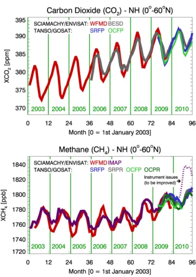
(Figure 1 top panel; see also Schneising et al., 2011, and references given therein; for a detailed 76
discussion of Fig. 1 see Sect. 4). An improved understanding of the CO2 sources and sinks is needed
77
for reliable prediction of the future climate of our planet (Solomon et al., 2007). This is also true for 78
methane (CH4, Figure 1 bottom panel). Atmospheric methane levels increased until about the year
79
2000, were rather stable during ~2000-2006, but started to increase again in recent years (Rigby et al., 80
2008, Dlugokencky et al., 2009, Schneising et al., 2011, Frankenberg et al., 2011). Unfortunately, it is 81
not well understood why methane was stable in the years before 2007 (e.g., Simpson et al., 2012) nor 82
why it started to increase again at a rate of approximately 7-8 ppb/year (Schneising et al., 2011). 83
Global satellite observations sensitive to near-surface CO2 and CH4 variations can contribute to a
84
better understanding of the regional sources and sinks of these important greenhouse gases. 85
Information on GHG surface fluxes (emissions and uptake) can be obtained by inverse modeling of 86
4
surface fluxes (e.g., Chevallier et al., 2007, Bergamaschi et al., 2009), where satellite observations are 87
compared with predictions of a (chemistry) transport model (e.g., Figure 2) and satellite minus model 88
mismatches are minimized by modifying the surface fluxes used by the model. This requires satellite 89
retrievals to meet challenging requirements, as small errors of the satellite-retrieved atmospheric GHG 90
distributions may result in large errors of the inferred GHG surface fluxes (e.g., Meirink et al., 2006, 91
Chevallier et al., 2005). Instead of direct optimization of surface fluxes it is also possible to optimize 92
(other) model parameters used to model the fluxes, as done in Carbon Cycle Data Assimilation 93
Systems (CCDAS) (e.g., Kaminski et al., 2010, 2012) or other approaches (e.g., Bloom et al., 2010). 94
The goal of the GHG-CCI project is to generate the Essential Climate Variable (ECV) Greenhouse 95
Gases (GHG) as defined by GCOS (Global Climate Observing System): “Distribution of greenhouse 96
gases, such as CO2 and CH4, of sufficient quality to estimate regional sources and sinks” (GCOS,
97
2006). In order to get information on regional GHG sources and sinks, satellite measurements must be 98
sensitive to near-surface GHG concentration variations. Currently only two satellite instruments 99
deliver (or have delivered until recently) measurements which fulfill this requirement: SCIAMACHY 100
on ENVISAT (March 2002 – April 2012) (Bovensmann et al., 1999) and TANSO-FTS on-board 101
GOSAT (launched in January 2009) (Kuze et al., 2009). Both instruments perform (or have 102
performed) nadir observations of reflected solar radiation in the near-infrared/short-wave-infrared 103
(NIR/SWIR) spectral region, covering the relevant absorption bands of CO2 and CH4. They also cover
104
the O2 A-band spectral region to obtain “dry-air columns” needed for computing GHG dry-air column
105
averaged mole fractions and/or to obtain information on clouds and aerosols. These two instruments 106
are therefore the two core sensors used by GHG-CCI and the near-surface-sensitive column-averaged 107
dry air mole fractions of atmospheric CO2 and CH4, denoted XCO2 (in ppm) and XCH4 (in ppb), are
108
the core data products of GHG CCI. In addition, other sensors or viewing modes are also used (e.g., 109
MIPAS/ENVISAT and SCIAMACHY solar occultation mode for stratospheric CH4 profiles and
110
IASI/METOP for mid/upper tropospheric CO2 and CH4 columns) as they provide additional
111
constraints for atmospheric layers above the planetary boundary layer. The focus of the first two years 112
5
of the GHG-CCI project (September 2010 – August 2012) was to develop existing retrieval algorithms 113
further, in order to improve the accuracy of the retrieved GHG data products. 114
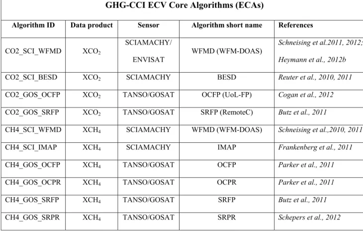
The focus of GHG-CCI lies on ECV Core Algorithms (ECAs) and their core data products XCO2 and
115
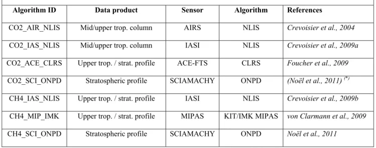
XCH4, which is also the focus of this manuscript. Other algorithms, referred to as Additional
116
Constraints Algorithms (ACAs), are algorithms to retrieve CO2 and/or CH4 information from satellite
117
data which have no or only little near surface sensitivity but are sensitive to GHG variations in upper 118
layers (the ACAs are listed in Table 3 and further discussed in Section 6). 119
Several existing candidate ECAs were selected at the outset of the project for ongoing development, 120
and have been iteratively improved upon through the course of the algorithm inter-comparison and 121
validation activity. This activity is referred to as “Round Robin” (RR) exercise within the CCI. 122
The goal of the RR was to determine which ECA performs best to generate a given GHG-CCI core 123
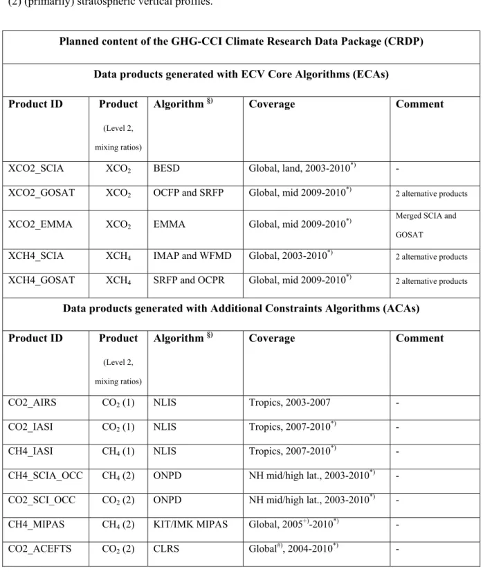
data product. The selected ECAs will be used in the third year of this project to generate the Climate 124
Research Data Package (CRDP), which will essentially be the first version of the ECV GHG. The 125
description of the RR approach and its results is the focus of this manuscript. Note that previous 126
publications focused on individual algorithms and their data product. Only recently have results 127
obtained using different algorithms been compared, most notably by Oshchepkov et al., 2012, for 128
TANSO/GOSAT XCO2. This manuscript is therefore one of the first focusing on inter-comparisons.
129
This manuscript is structured as follows: Section 2 presents an overview of the GHG-CCI project 130
followed by a description of the user requirements in Section 3. In Section 4 the retrieval algorithms 131
are briefly described. The main part of this manuscript is Section 5 where the RR approach and its 132
main results are presented and discussed. Section 6 provides a short overview of the Additional 133
Constraints Algorithms (ACAs) also used within GHG-CCI but not the focus of this manuscript. 134
Section 7 gives a short overview of the Climate Research Data Package (CRDP) to be generated using 135
the selected algorithms. A summary and conclusions are given in Section 8. 136
6 2. GHG-CCI project overview
137
The GHG-CCI project covers all aspects needed to generate the ECV GHG and to assess its quality 138
and usefulness. This includes the use of appropriate satellite instruments (primarily 139
SCIAMACHY/ENVISAT and TANSO/GOSAT to generate global XCO2 and XCH4 time series),
140
calibration aspects (related to "Level 0-1 processing", primarily for SCIAMACHY), and development 141
and application of retrieval algorithms to convert the satellite-measured spectra into atmospheric CO2
142
and CH4 information ("Level 1-2 processing"). Also included is the analysis of the resulting global
143
data sets, including validation and user assessments, focusing on inverse modeling of regional surface 144
fluxes (i.e., "Level 2-4 processing"). Note that the fluxes (Level 4 products) will most likely be 145
derived from Level 2 data rather than from (spatio-temporally averaged and potentially gap-filled) 146
Level 3 data products, as Level 2 data contain more information than those at Level 3 and usually 147
benefit from better error characterization. 148
Level 1 data (i.e., geolocated and calibrated radiances) are input data for CCI (i.e., Level 0-1 149
processing is covered by other projects). SCIAMACHY Level 0-1 processing experts are part of the 150
GHG-CCI team in order to provide expertise and to ensure that the findings of the study feed back to 151
improve future Level 1 data products if necessary. Close links have been established with the GOSAT 152
team at JAXA for GOSAT Level 1 data access, expertise and feedback. 153
The SCIAMACHY and TANSO Level 1 data products are de-facto used as Fundamental Climate Data 154
Records (FCDRs, see GCOS, 2006) despite the fact that no dedicated inter-calibration or merging 155
efforts are currently foreseen. Consistency between the time series of the two GHG-CCI core satellites 156
is addressed at the level of the Level 2 data products. Ideally, an ECV data product or Thematic 157
Climate Data Record (TCDR) of a given quantity should be a single merged data record obtained from 158
all available appropriate sensors such as SCIAMACHY and TANSO for satellite-derived XCO2.
159
However, within the present initial stage of this project only first steps in this direction have been 160
carried out (see Section 5). 161
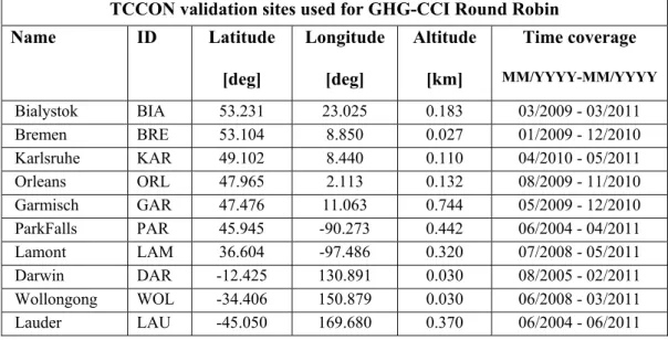
The ground-based validation of the “satellite-derived” XCO2 and XCH4 data products largely relies on
162
the Total Carbon Column Observing Network (TCCON) (Wunch et al., 2010, 2011a) as this network 163
7
has been designed and developed for this purpose. Methods to also use data from other sources in the 164
future (e.g., NDACC (see Sussmann et al., 2013), GAW) are being developed in parallel. Aircraft 165
observations, e.g., HIPPO (e.g., Wofsy, 2011, Wecht et al., 2012), are also interesting, but have not yet 166
been used directly (indirectly some of these data have been used via the calibration of TCCON, see 167
Sect. 5.2.1). 168
A dedicated GHG-CCI Climate Research Group (CRG) has been set up to represent the users of the 169
satellite-derived CO2 and CH4 data products and to provide expertise on inverse modeling of surface
170
fluxes, CCDAS and other user related aspects. A strong link exists between GHG-CCI and the EU FP7 171
GMES project MACC-II (Monitoring of Atmospheric Composition and Climate - Interim 172
Implementation, http://www.gmes-atmosphere.eu/) that provides feedback on the data quality. 173
Key activities carried out in the first two years of this project were the establishment of the user 174
requirements (Section 3), the further development of retrieval algorithms (described briefly in Section 175
4) and data processing and data analysis with the goal of identifying which algorithms perform best 176
(“Round Robin” (RR)). The description of these RR activities and their results is the focus of this 177
manuscript (Section 5). In the third year of this project the selected algorithms will be used to generate 178
the CRDP (see Section 7), which will subsequently be validated and assessed by users. 179
3. User requirements 180
An important initial activity carried out in this project was the establishment of the user requirements. 181
They have been formulated in detail in the GHG-CCI User Requirements Document (URD) (Buchwitz 182
et al., 2011a). The requirements are based on peer-reviewed publications primarily prepared in the 183
context of existing or planned satellite missions and GHG-CCI CRG user expertise and experience 184
with existing satellite data. 185
Most critical are the requirements on random and systematic errors listed in Table 1. The most 186
challenging requirement is the one on biases for XCO2. The threshold requirement is 0.5 ppm because
187
even errors of a few tenths of a ppm can result in large errors of the inferred CO2 surface fluxes when
188
used as input data for inverse modeling schemes (e.g., Chevallier et al., 2005). However, to what 189
8
extent systematic errors result in biases of the inferred fluxes depends on the spatio-temporal pattern 190
of the systematic errors. A global bias, even if considerably larger than the required 0.5 ppm, would 191
not be critical because it can easily be detected and corrected ad hoc. Most critical are state-dependent
192
systematic errors, which result in regional-scale (~1000 km) biases on medium time scales (~ 193
monthly), because they will likely be missed by bias-correction schemes. As the overall impact of the 194
atmospheric concentration error on the surface flux error depends on the spatio-temporal pattern of the 195
concentration error, the values listed in Table 1 have to be interpreted with care. The requirements 196
reflect what the GHG-CCI users would like to see achieved. The utility of the data can ultimately only 197
be determined by careful analysis. The numbers listed in Table 1serve to give a rough indication of the 198
required uncertainties but should not be over-interpreted. 199
The requirements for XCH4 are also challenging but somewhat less demanding than those for XCO2.
200
The main reason is that XCH4 is more variable compared to XCO2 relative to its background value on
201
the spatio-temporal scales relevant for the satellite retrievals (e.g, Frankenberg et al., 2005, 2011, 202
Meirink et al., 2006, Bergamaschi et al., 2009, Schneising et al., 2011, 2012). 203
4. Retrieval algorithms 204
In this section, a brief overview of each retrieval algorithm used for the GHG-CCI RR is given. The 205
reader is referred to peer-reviewed publications for details. All algorithms used within the GHG-CCI 206
RR are also described in the GHG-CCI Algorithm Theoretical Basis Document (ATBD) (Reuter et al., 207
2012a). 208
The ECV Core Algorithms (ECAs) generate one or more of the four GHG-CCI core data products, 209
XCO2 (in ppm) and XCH4 (in ppb) from SCIAMACHY and TANSO (each of the four combinations is
210
a separate product). An overview of these algorithms is given in Table 2 and briefly described in the 211
following sub-sections. Results obtained with all ECAs are shown in Fig. 1: the top panel shows 212
northern hemispheric (NH) time series of XCO2 and the bottom panel XCH4 time series. As can be
213
seen, the various XCO2 time series (generated with the various algorithms described in the following
214
sub-sections) are similar but not exactly identical. There are clear differences, e.g., a difference of the 215
seasonal cycle amplitude, between the two SCIAMACHY algorithms WFMD (Schneising et al., 2011, 216
9
Heymann et al., 2012b) and BESD (Reuter et al., 2011) likely due to sub-visual cirrus clouds not 217
explicitly considered by WFMD. Differences are also due to the different spatial sampling of the 218
various data products. From Figure 1 it can therefore typically not be concluded which data product is 219
the most accurate. This requires, for example, a careful comparison with independent accurate ground-220
based observations (see Section 5.2). However, one obvious problem can be identified: the 221
SCIAMACHY XCH4 product generated with the IMAP algorithm (Frankenberg et al., 2011) suffers
222
from a significant high bias (relative to several other TANSO/GOSAT XCH4 data products) during the
223
year 2010 (highlighted by the dotted line). This problem is related to SCIAMACHY detector 224
degradation issues which are not yet properly dealt with by the SCIAMACHY radiometric calibration 225
nor compensated by the IMAP algorithm (note that the second SCIAMACHY XCH4 algorithm
226
WFMD (Schneising et al., 2011) has not yet been applied to 2010 data; the WFMD time series covers 227
only the years 2003-2009). As will be discussed in more detail below, the most challenging problems 228
addressed within GHG-CCI are related to achieving the required accuracy: for XCO2 this is a
229
challenge because of demanding user requirements and for XCH4 the most important challenge was to
230
deal with the progressive SCIAMACHY detector degradation in the spectral region needed for 231
methane retrieval which started in October 2005 (see Schneising et al., 2011, and Frankenberg et al., 232
2011, for a detailed discussion). 233
4.1 Full Physics (FP) and Proxy (PR) algorithms 234
Within GHG-CCI, two types of ECAs can be distinguished: The “Full Physics” (FP) algorithms and 235
the light path “Proxy” (PR) algorithms (see also Schepers et al., 2012). 236
FP algorithms model all relevant physical effects such as scattering by aerosols and clouds and have 237
corresponding elements as part of the state vector, which contains all parameters which are to be 238
retrieved. The FP algorithms obtain the dry air column-averaged mole fraction (needed to compute the 239
dry air column-averaged mole fractions of the GHG, i.e., XCO2 and/or XCH4) either from the
240
retrieved surface pressure or using meteorological information. 241
10
The PR algorithms are based on computing the dry air column-averaged mole fraction using a 242
“reference gas”, which has to be much less variable than the gas of interest on the relevant spatio-243
temporal scales. The PR method is used for XCH4 retrieval using CO2 as a reference gas. The XCH4 is
244
essentially obtained from computing the ratio of the retrieved CH4 column and the retrieved CO2
245
column. The advantage of this method is that it is potentially very fast, accurate and robust (as several 246
systematic errors cancel in the CH4/CO2 column ratio). The disadvantage is that a correction is needed
247
for CO2 variability, typically based on a global model (see, e.g., Frankenberg et al., 2005, 2011, Parker
248
et al., 2011, Schneising et al., 2009, 2011, Schepers et al., 2012). 249
4.2 SCIAMACHY XCO2 algorithms
250
The Weighting Function Modified (WFM) Differential Optical Absorption Spectroscopy (DOAS) 251
algorithm (WFM-DOAS or WFMD) has been developed to retrieve vertical columns of several 252
atmospheric gases including the GHGs discussed in this manuscript (Buchwitz et al., 2000). During 253
the last decade, this algorithm has been significantly improved and used to generate global multi-year 254
XCO2 and XCH4 data sets from SCIAMACHY (Buchwitz et al., 2005, 2007; Schneising et al., 2008,
255
2009). Within GHG-CCI, WFMD has been further improved and used to generate long-term 256
consistent time series (Schneising et al., 2011, 2012, Heymann et al., 2012a, 2012b). WFMD has been 257
implemented as a fast look-up table (LUT) based retrieval scheme to avoid time consuming radiative 258
transfer (RT) simulations. WFMD is a least-squares method using a single constant atmospheric prior 259
(e.g., single constant CO2 and CH4 mixing ratio profiles, a single aerosol scenario, no clouds). WFMD
260
can process one orbit of SCIAMACHY observations in a few minutes on a single workstation. 261
Aerosols and cirrus clouds are only treated approximately by considering spectrally broad band effects 262
by a low-order polynomial and by post-processing filtering. Overall, this results in small but 263
significant biases, especially for XCO2 (Heymann et al., 2012a). Recently, an improved version of
264
WFMD has been developed for SCIAMACHY XCO2 retrieval (Heymann et al., 2012b, see also
265
Figure 2) and the XCO2 data set generated with this latest version has been used for the GHG-CCI RR.
266
For SCIAMACHY XCH4 retrieval, the WFMD version described in Schneising et al., 2011, 2012, has
267
been used (see below). 268
11
The Bremen Optimal Estimation DOAS (BESD) FP algorithm was specifically developed for accurate 269
and precise SCIAMACHY XCO2 retrieval considering aerosols and clouds thereby overcoming
270
limitations of the WFMD algorithm (Reuter et al., 2010, 2011). In contrast to WFMD, BESD is not 271
based on a LUT scheme but uses on-line RT model simulations. BESD is therefore computationally 272
much more demanding. Also, unlike WFMD, BESD is based on Optimal Estimation (OE, Rodgers, 273
2000) and aerosol and cirrus parameters are state vector elements and retrieved in addition to XCO2.
274
4.3 TANSO XCO2 algorithms
275
Both GHG-CCI TANSO XCO2 retrieval algorithms are FP algorithms: the University of Leicester’s
276
(UoL) OCO (Orbiting Carbon Observatory, Crisp et al., 2004) FP (“UoL-FP” or OCFP) algorithm 277
(Cogan et al., 2012, Parker et al., 2011) and the RemoteC (or SRON Full Physics (SRFP)) algorithm 278
(Butz et al., 2011). Both algorithms are based on adjusting parameters of a surface-atmosphere state 279
vector and other parameters to the satellite observations, but differ in many details (different RT 280
models, different inversion schemes (OE or Tikhonov-Phillips), different schemes for aerosol 281
modeling and inversion, use of different pre-processing and post-processing steps, etc.) as discussed in 282
Cogan et al., 2012, Parker et al., 2011, and Butz et al., 2011. 283
4.4 SCIAMACHY XCH4 algorithms
284
For SCIAMACHY XCH4 retrievals, PR algorithms are used: WFMD (Schneising et al., 2011, see
285
above) and IMAP (Iterative Maximum A Posteriori) DOAS (Frankenberg et al., 2011). These 286
algorithms were already well developed when GHG-CCI started but had essentially only been applied 287
to retrieve XCH4 from the first three years of the ENVISAT mission (e.g., Schneising et al., 2008).
288
Within GHG-CCI, this time series has been significantly extended. The key challenge was (and partly 289
still is, see Figure 1) to deal with the significant detector degradation in the spectral region needed for 290
methane retrievals after 2005 (see Frankenberg et al., 2011, and Schneising et al., 2011, for details). 291
12 4.5 TANSO XCH4 algorithms
292
To overcome the key limitation of the XCH4 PR algorithms, namely the need to correct the retrieved
293
XCH4 for CO2 variations using a model, FP algorithms are also used within GHG-CCI, but only for
294
TANSO. TANSO has higher spectral resolution than SCIAMACHY which is exploited to also retrieve 295
scattering parameters in addition to CH4. Two TANSO XCH4 FP retrieval algorithms are being used
296
within GHG-CCI, which are also used for TANSO XCO2 retrieval (see above), OCFP (Parker et al.,
297
2011) and SRFP (Butz et al., 2011), in addition to the two PR algorithms OCPR (Parker et al., 2011) 298
and SRPR (Schepers et al., 2012). 299
5. Round Robin approach and results 300
In this section an overview of the GHG-CCI Round Robin (RR) activities is given which have been 301
carried out in the first two years of this project. 302
5.1 Round Robin approach 303
The ultimate goal of the GHG-CCI RR was to identify which algorithms and corresponding data 304
products to use for generating the CRDP. This comprised the further development of existing retrieval 305
algorithms with the goal of meeting the challenging user requirements, the application of these 306
algorithms to generate global multi-year XCO2 and XCH4 sets, the comparison with ground-based
307
reference data and inter-comparisons of the data products generated with the competing ECAs. 308
The selection procedure for ECAs and ACAs is described in the GHG-CCI Round Robin Evaluation 309
Protocol (RREP, Buchwitz et al., 2011b). Initially the plan was to develop a score-based selection 310
scheme, i.e., to compute a single number for each algorithm / data product (the higher the number, the 311
better the algorithm), mainly based on satellite – ground-based observation differences. However, this 312
was not pursued because a scientifically sound basis for the classification could not be established. 313
Instead a set of Figures of Merit (FoM), mostly based on differences between satellite and ground-314
based observations, have been defined (see RREP, Buchwitz et al., 2011b) and evaluated. However, as 315
explained in the RREP and also shown in this manuscript, the comparison with the ground-based 316
observations is only one component for the final selection primarily because of the sparseness of the 317
13
ground-based network (see Section 5.2). Another major component of the selection procedure was the 318
analysis of (global and regional) maps and time series, including comparisons with global state-of-the-319
art models, and inter-comparisons of the data products generated with the different candidate 320
algorithms. Note that “blind testing” has not been used as it would have been possible to identify the 321
algorithms/products by using some of their characteristics such as averaging kernels and spatial 322
coverage. Some key results of this RR activity are presented here including a summary of the main RR 323
decision results given in Section 5.6 for ECAs and Section 6 for ACAs. 324
According to the initial ESA specification of the CCI RR exercise it was required to evaluate 325
“algorithms”. However, complex algorithms such as the ones used within GHG-CCI can hardly be 326
evaluated, especially not in terms of identifying “the best one” in terms of smallest biases when 327
applied to real data. Simulated retrievals have been performed (see, e.g., Buchwitz et al., 2011c, 328
2012a, and references given therein) but only for the individual algorithms and not in a consistent 329
manner. This would have been a major activity incompatible with the CCI schedule especially if the 330
goal would have been to obtain a better understanding of the differences between the data products 331
obtained from the real observations. In this context it has not been identified that any of the algorithms 332
suffer from obvious shortcomings. All XCO2 algorithms, for example, use different approaches to
333
mitigate biases due to scattering by aerosols and (thin) clouds, but it is virtually impossible to identify 334
a priori, e.g., based on a description of the algorithms and the simulation results, which of the
335
approaches will result in the smallest XCO2 or XCH4 biases when applied to real data.
336
What has been evaluated in detail are the end products, i.e., the quality of the XCO2 and XCH4 data
337
products. This means that primarily data products have been evaluated during RR but not algorithms. 338
As shown in this manuscript, this is not a trivial task, e.g., due to the sparseness of the TCCON 339
reference data. Therefore, as shown in this manuscript, the RR decisions are not only based on 340
comparisons with TCCON. The satellite retrieval team focused on producing the best possible end 341
products. Which input data to use and how to treat them, e.g., in a dedicated pre-processing step, has 342
not been prescribed. Pre-processing steps may be critical for the quality of the end product. This is 343
particularly true if the instrument shows significant degradation as is the case for SCIAMACHY after 344
14
2005 especially in the spectral region needed for methane retrieval. To deal with this, quite different 345
approaches have been used by the two algorithms IMAP (Frankenberg et al., 2011) and WFMD 346
(Schneising et al., 2011, 2012). For example, IMAP uses as input data spectra that have been 347
specifically calibrated at SRON and IMAP also uses a single so-called “Dead and Bad detector Pixel 348
Mask” (DBPM), needed to reject detector pixels which are not useful. In contrast, WFMD uses the 349
official standard SCIAMACHY Level 1 data product with standard calibration and several DBPMs, 350
each optimized for a certain time period, typically covering one or more years (see Schneising et al., 351
2011, for details). 352
Finally, it is important to highlight the preliminary nature of the RR. This is due to the fact that all 353
Level 1 input data and retrieval algorithms are continuously being improved. An algorithm / data 354
product currently identified to be the best one will not necessarily be the best one in the future. GHG-355
CCI therefore needs to be flexible and will aim to consider this in future phases of the CCI. 356
5.2 Comparison with ground-based (TCCON) observations 357
5.2.1 TCCON data and error characteristics 358
The most relevant ground-based observations for the validation of the satellite-derived XCO2 and
359
XCH4 data products are the corresponding data products of the TCCON. The TCCON data products
360
have been obtained from the TCCON website (www.tccon.caltech.edu/; latest access Feb. 2012 using 361
version GGG2009, i.e., not the latest version GGG2012, which was not available for the GHG-CCI 362
Round Robin comparison) or have been provided by the TCCON PIs. The TCCON products have 363
been calibrated to WMO/GAW in situ trace gas measurement scales using aircraft observations 364
(Wunch et al., 2010, Deutscher et al., 2010, Geibel et al., 2012, Messerschmidt et al., 2012). The best 365
independent estimates of the TCCON inter-site comparability to date are provided by these 366
independent aircraft calibration data. While not exhaustive, these demonstrate consistency at the 0.1% 367
level (1-sigma) for XCO2 (~0.4 ppm) and 0.2% for XCH4 (~4 ppb), with no obvious inter-hemispheric
368
differences (Wunch et al., 2010). Nevertheless, the TCCON team recognizes that inter-site 369
comparability needs to be better characterized, especially for methane (e.g., at Darwin and 370
Wollongong, not discussed in the references cited above), and work is in progress to achieve this. The 371
15
systematic and random errors of single TCCON data are therefore typically 0.4 ppm for XCO2
(1-372
sigma) and 4 ppb (1-sigma) for XCH4 (Notholt et al., 2012, based on Wunch et al., 2010). Due to these
373
errors of the TCCON data (but also for other reasons, e.g., non-perfect spatio-temporal co-location) 374
the estimated systematic and random errors of the satellite retrievals as reported here have to be 375
interpreted as upper limit estimates, i.e., the satellite data errors are likely smaller than reported here. 376
5.2.2 Inter-comparison method 377
Different inter-comparison methods have been used, e.g., to ensure robustness of the findings. In 378
addition to the method used and results obtained by the validation team (Notholt et al., 2012), which 379
are summarized in this manuscript, independent inter-comparisons of the satellite data products with 380
TCCON have also been carried out by the satellite data product provider (Buchwitz et al., 2012a). The 381
methods differ by various aspects such as investigated time period and direct comparison or 382
comparison after transformation to common a priori profiles and application of averaging kernels.
383
Each satellite data product provider performed an independent validation of his data product 384
(considering averaging kernels or not) covering the entire time series (to the extent possible given the 385
limitations of the TCCON data, see Tab. 4). In contrast, the validation team has applied the same 386
method to all satellite data products and has, for a given product, only used a time period where data 387
from all competing algorithms were available (SCIAMACHY: XCO2: 2006-2009; XCH4: 2003-2009,
388
TANSO: mid 2009-2010). 389
The method used by the validation team is based on a direct comparison of the co-located satellite and 390
TCCON data products. No correction for different a priori profiles and averaging kernels has been
391
applied. Note that it is not trivial to consider averaging kernels for the XCO2 and XCH4 satellite and
392
TCCON retrievals as strictly speaking this requires a reliable estimate of the real atmospheric 393
variability, which is unknown. This aspect is discussed in detail in Wunch et al., 2011b, where the 394
impact of this correction for TANSO XCO2 is discussed at Lamont, USA, where the real variability of
395
the CO2 profiles is obtained using regular aircraft and other observations. For the global data sets this
396
is not possible. Nevertheless, for some of the satellite products, averaging kernels have been applied 397
by the satellite data provider. For example, Reuter et al., 2013, has applied individual averaging 398
16
kernels for all XCO2 products from SCIAMACHY and TANSO by adjusting all retrievals to a
399
common a priori using the Simple Empirical CO2 Model (SECM) described in Reuter et al., 2012b.
400
They found that the adjustments are typically a few tenth of a ppm. Reuter et al., 2012b, estimated the 401
smoothing errors and found that it is typically 0.17 ppm for SCIAMACHY XCO2 and 0.05 ppm for
402
TCCON XCO2. These results indicate that the impact of applying or not applying the averaging
403
kernels for satellite – TCCON comparisons is small. The reason is that the averaging kernels of the 404
TCCON and the satellite data are close to unity and the resulting smoothing error is therefore typically 405
quite small, especially for XCO2. For methane the (relative) smoothing errors are somewhat larger, as
406
methane is more variable. For example, Parker et al., 2011, found that “the mean smoothing error 407
difference included in the GOSAT to TCCON comparisons can account for 15.7 to 17.4 ppb for the 408
northerly sites and for 1.1 ppb at the lowest latitude site”. For the SCIAMACHY XCH4 validation
409
results presented in Schneising et al., 2012, it has been found that applying averaging kernels (by 410
using TM5 model profiles as a common a priori) leads to adjustments of 0.4% (approx. 7 ppb).
411
Overall it has been found that the validation results obtained by the validation team (Notholt et al., 412
2012) and the satellite data provider (Buchwitz et al., 2012a), where averaging kernels have been 413
applied for at least some of the products, agree well, especially for XCO2 (Buchwitz et al., 2012b).
414
The comparison of the various methods used to quantify random and systematic errors of the satellite 415
products (Buchwitz et al., 2012b) indicates that the RR validation results are robust. 416
In the following, the results obtained by the validation team are presented. Detailed results will be 417
reported elsewhere (Dils et al., manuscript in preparation, preliminary title: “The Greenhouse Gas 418
Climate Change Initiative (GHG-CCI): Comparative validation of SCIAMACHY and TANSO-FTS 419
CO2 and CH4 retrieval algorithm products with measurements from the TCCON network”). Therefore
420
we here give only a short overview highlighting major findings. 421
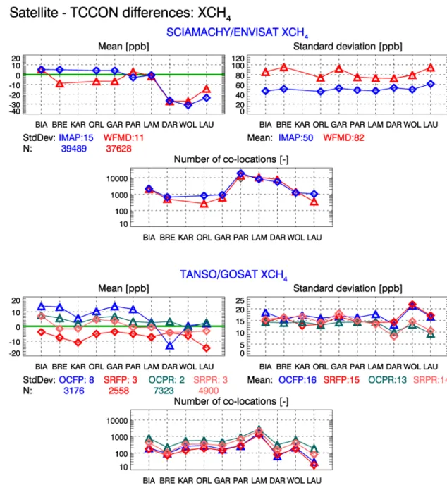
For each product and each TCCON site a number of Figures of Merit (FoMs) have been computed by 422
the validation team. Key results are shown in Fig. 3 for XCO2 and Fig. 4 for XCH4., discussed in detail
423
in dedicated sub-sections below. Shown are comparisons of the four GHG-CCI core data products 424
generated with two or more of the candidate algorithms at the 10 TCCON sites listed in Table 4. The 425
17
results shown in Figs. 3 and 4 have been generated using a spatio-temporal co-location criterion of 2 426
hours and 500 km (for alternative co-location criteria see Notholt et al., 2012). Several numerical 427
values are given, which are also listed in Table 5, computed from satellite minus TCCON differences 428
for each single satellite retrieval and the corresponding TCCON mean value. On the left hand side of 429
Figs. 3 and 4 the mean satellite-TCCON differences are shown for each of the 10 TCCON sites and all 430
four core data products and their corresponding ECAs. For each ECA the standard deviation of the 431
station-to-station bias has been computed (“StdDev”) and the total number of co-located satellite 432
retrievals used for comparison (“N”). The standard deviation of the station-to-station bias is 433
interpreted as a relevant measure of the systematic error (“relative accuracy” or “relative bias”). The 434
standard deviation is more relevant to characterize systematic errors compared to, for example, the 435
mean difference. Most critical is to achieve high “relative accuracy” (or low “relative bias”) not 436
necessarily high “absolute accuracy” (although this would of course be better). For example, a 437
constant offset of the satellite data would not be critical if the data are being used for surface flux 438
inverse modeling (see Section 3) and this is considered by computing the standard deviation. On the 439
right hand side of Figs. 3 and 4 the standard deviations of the satellite-TCCON differences are shown 440
for each TCCON site. They are a measure of the random error (scatter) of the satellite retrievals. The 441
corresponding mean value over all TCCON sites is used to characterize the mean random error (or 442
“precision”) of the corresponding satellite data product. In the following, Figs. 3 and 4 are discussed in 443
more detail for each of the products. 444
5.2.3 Satellite XCO2 comparisons with TCCON
445
The comparison of the two SCIAMACHY XCO2 retrieval algorithms WFMD and BESD with
446
TCCON shows the following (Figure 3, top half): BESD has typically lower systematic errors (0.7 447
ppm) compared to WFMD (1.3 ppm) and also a higher precision (2.3 ppm compared to 5.1 ppm). 448
Ultimately it can be expected that the biases of BESD will be even lower as it has been identified (not 449
shown) that the BESD RR data set suffers from problems related to the SCIAMACHY Level 1 data 450
product used (version 7 consolidation level u, “L1v7u”). This data product was used because it was the 451
latest version available when the final RR data set had to be generated and because it also covers the 452
18
time period after 2009. The previous Level 1 version 6 (L1v6), used by WFMD, does not suffer from 453
these problems but is only available until the end of 2009, where the WFMD data set ends. It has been 454
found that BESD retrievals for selected months using the improved new version L1v7w have much 455
lower biases especially because the many outliers caused by the L1v7u spectra are not present any 456
more (not shown). It is therefore necessary and planned to reprocess the entire SCIAMACHY data set 457
with BESD using L1v7w, e.g., for the generation of the CRDP. A potentially important pro for 458
WFMD for certain applications is the much larger number of data points. 459
The comparison of the two TANSO XCO2 retrieval algorithms OCFP and SRFP with TCCON shows
460
the following (Figure 3, bottom half): The biases depend on site and are typically in the range +/- 1 461
ppm. They are very similar for both algorithms. This is also true for the standard deviation of the 462
difference between the TANSO and TCCON estimates, which is typically in the range 2-3 ppm. The 463
number of co-locations is also nearly identical for both algorithms but varies significantly from site to 464
site, which is true for all comparisons shown in Figs. 3 and 4. 465
As shown in Table 5, the precision requirement for XCO2 is met by all algorithms. WFMD meets the
466
threshold requirement and the other algorithms including BESD even meet the breakthrough 467
requirement. The challenging 0.5 ppm bias requirement has however not yet been met but several 468
algorithms achieve a performance close to the threshold requirement (0.6-0.9 ppm, depending on 469
algorithm). 470
5.2.4 Satellite XCH4 comparisons with TCCON
471
The comparison of the two SCIAMACHY XCH4 retrieval algorithms WFMD and IMAP with
472
TCCON shows the following (Figure 4, top half): Overall, the systematic differences with respect to 473
TCCON vary from site to site from nearly 0 ppb at Lamont to 20-30 ppb at the southern hemisphere 474
(SH) sites Darwin, Wollongong, and Lauder, but are very similar for WFMD and IMAP. The reason 475
for the large differences at these SH sites have not yet been identified. This is probably not due to the 476
TCCON reference data as these differences are larger than the estimated TCCON inter-site 477
comparability (see Sect. 5.2.1) and also the comparison with TANSO XCH4 (see below) does not
478
show this type of systematic deviation (the OCFP results however also show a low bias at the SH sites 479
19
compared to the northern sites esp. at Darwin). Agreement is within +/- 10 ppb if these SH sites are 480
excluded. In order to obtain an estimate of the relative biases (i.e., considering that an overall offset is 481
not critical), the standard deviation of the station-to-station biases has been computed: it amounts to 11 482
ppb for WFMD and 15 ppb for IMAP. The standard deviation of the satellite-TCCON differences, 483
which is a measure of the single measurement precision (1-sigma), is on average 82 ppb for WFMD 484
and 50 ppb for IMAP. Because nearly all TCCON sites started operation after 2005 (see Table 4), i.e., 485
after the loss of important SCIAMACHY methane detector pixels due to detector degradation, the 486
values listed for SCIAMACHY in Figure 4 are not representative for the years 2003-2005. Until the 487
end of 2005 the performance was much better and the corresponding values are listed in curved 488
brackets in Table 5. A possible explanation for the larger scatter (worse precision) of WFMD after 489
2005 is that WFMD is an unconstrained least-squares algorithm whereas IMAP is based on Optimal 490
Estimation and uses detailed CH4 information (as a function of latitude, altitude and time but not
491
longitude) from a global model as a priori information. This raises the question why the precision of
492
the two data products is similar for 2003-2005. This could be related to the fact that only a single 493
DBPM is used by IMAP whereas WFMD has used a DBPM optimized for 2003-2005. Another 494
possible explanation could be the use of differently calibrated input data. As shown in Fig. 4, the 495
number of satellite soundings used varies significantly from site to site, but overall is very similar for 496
WFMD (N=37628) and IMAP (39489) (at least at TCCON sites, for other locations this may not be 497
true, see Figures 9 and 10). 498
The comparison of the four TANSO XCH4 retrieval algorithms (OCPR, OCFP, SRPR, SRFP) with
499
TCCON shows the following (Figure 4, bottom half): The biases depend on the TCCON site but are in 500
the range +/- 15 ppb. The estimated relative bias is best for OCPR (2 ppb) and worst for OCFP (8 501
ppb). OCPR has the largest number of data points (followed by SRPR). The number of data points is 502
higher for the PR algorithms (OCPR and SRPR) compared to the FP algorithms (OCFP and SRFP). 503
The FP algorithm with the lowest relative bias is SRFP (3 ppb). The PR algorithm with the lowest 504
relative bias is OCPR (2 ppb). The standard deviation of the satellite – TCCON differences are nearly 505
identical for all four algorithms. 506
20
As shown in Table 5, the SCIAMACHY XCH4 product for 2003-2005 meets the threshold precision
507
requirement (but not for 2006 and later years due to the detector degradation). In contrast, the TANSO 508
XCH4 has a much higher precision and even the breakthrough precision requirement is met by all
509
algorithms. All TANSO XCH4 algorithms meet the relative accuracy (relative bias) user requirement -
510
some are close to or even better than the goal requirement. For SCIAMACHY this is only true for 511
2003-2005. 512
Concerning the final RR algorithm selection decision, it is important not to over-interpret the 513
numerical values listed in Table 5 due to the sparseness of the TCCON sites. For this and other 514
reasons, the TCCON comparisons presented and discussed in this section are only one key component 515
of the GHG-CCI RR activities. Therefore, more comparisons have been conducted, for XCO2 and
516
XCH4, as described in the following.
517
5.3 Inter-comparison of XCO2 data products
518
Within GHG-CCI two algorithms have been further developed to retrieve XCO2 from SCIAMACHY,
519
namely WFMD and BESD, and two algorithms to retrieve XCO2 from TANSO, namely OCFP and
520
SRFP. In addition, there are three non-European TANSO algorithms presented and discussed in the 521
peer-reviewed literature whose data products have also been used for comparison: (i) the official 522
operational TANSO algorithm (v02.xx) developed at the National Institute for Environmental Studies 523
(NIES) in Japan (Yoshida et al., 2011; in the following referred to as “NIES” algorithm), (ii) a 524
scientific algorithm called PPDF (Pathlength Probability Density Function) also developed at NIES 525
(Bril et al., 2007, Oshchepkov et al., 2008, 2009, 2011, 2012), and (iii) NASA/JPL’s ACOS 526
(Atmospheric CO2 Observations from Space) v2.9 algorithm (O’Dell et al., 2012, Crisp et al., 2012).
527
The global XCO2 data products from all 7 algorithms have been inter-compared within GHG-CCI
528
(Reuter et al. 2013, Buchwitz et al., 2012a). The analysis revealed the following: The various satellite 529
XCO2 data products all capture the expected large scale variations of atmospheric CO2 such as the
530
time dependent north-south gradient (Figures 5 and 6, discussed below) and the CO2 increase and
531
seasonal cycle (Figure 1) but exhibit differences in the spatio-temporal pattern which – depending on 532
region and time – may exceed the relative bias user requirement of 0.5 ppm. 533
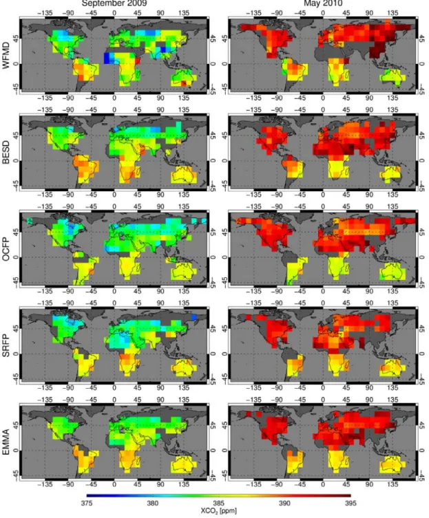
21
Typical examples are shown in Figures 5 and 6. Figure 5 shows comparisons of the four GHG-CCI 534
XCO2 algorithms (BESD, WFMD, SRFP, OCFP). Figure 6 shows the GHG-CCI algorithms as well as
535
the three non-European algorithms mentioned above (ACOS (v2.9), PPDF (NIES PPDF-D), and NIES 536
(v02.xx)) for the two months September 2009 and May 2010. Also shown is the ensemble data 537
product generated with the EnseMble Median Algorithm (EMMA) algorithm, discussed below, 538
TCCON XCO2, and XCO2 from NOAA’s CO2 assimilation system CarbonTracker (CT) (Peters et al.,
539
2007). As can be seen, all satellite retrieval algorithms capture the north-south XCO2 gradient, which
540
is significantly different for the two months shown, in good to reasonable agreement with TCCON and 541
CarbonTracker (Figure 6). As can also be seen, differences between the data products often exceed 0.5 542
ppm, particularly at locations remote from TCCON sites (e.g., Sahara, South America, Africa). As 543
discussed in Section 5.2, it appears virtually impossible to use TCCON to determine which algorithm 544
performs best, at least for TANSO. For SCIAMACHY it has been shown that BESD outperforms 545
WFMD in terms of single measurement precision and bias not however in terms of number of 546
observations, which is significantly higher for WFMD. It is also likely that a “best data product” for 547
all conditions does not exist at present as each retrieval algorithm is expected to have its strengths and 548
weaknesses. Therefore, which algorithm performs best may depend on the spatio-temporal interval of 549
interest. Clearly, more research is needed to understand the differences between the various XCO2 data
550
sets shown in Figures 5 and 6. One approach to further assess the relative quality of the various 551
satellite-derived global XCO2 data sets is to compare them with their median. This approach is
552
presented in the following section. 553
5.3.1 Comparison with ensemble median (EMMA) 554
In this section we aim at answering two related questions: (i) How to determine which data product is 555
likely “the best”, if the largest differences are at locations remote from validation sites? (ii) Which data 556
product should be used for inverse modeling of surface fluxes if all products differ and if it is not clear 557
which product would give the most reliable results? To answer these questions we use the median of 558
the various XCO2 products. The situation appears to be similar to that for climate modeling: it is not
559
clear which “model” is the best and (remote from validation sites) there is no truth to compare with. A 560
22
promising approach to deal with this is to make use of the fact that several state-of-the-art algorithms 561
and corresponding XCO2 data products are available, i.e., an ensemble of data products, which can be
562
exploited. This is the underlying idea of the EnseMble Median Algorithm (EMMA, Reuter et al., 563
2013). As described in more detail below and in Reuter et al., 2013, EMMA computes the median of 564
an ensemble of individual XCO2 data products, which can be used for comparison with the individual
565
data products, e.g., to identify outliers. However, the EMMA XCO2 product has also been generated to
566
be useful as a stand-alone XCO2 data product for inverse modeling and other applications.
567
The strength of using an ensemble of satellite data products was highlighted at the end of the first year 568
of the GHG-CCI project (Buchwitz et al., 2011c), when biases (0.5%) between Bialystok TCCON 569
XCO2 and co-incident satellite data were identified in the majority of algorithms participating in the
570
GHG-CCI. This bias occurred due to an empirical correction of known magnitude, to account for a 571
laser-sampling bias in the FTS data before September 21, 2009, inadvertently being applied in the 572
wrong direction. A bias in XCH4 in the early part of the Bialystok time series that occurred due to
573
missing fits in one of the CH4 micro-windows was also brought to light by comparisons to the
574
ensemble of satellite retrievals. The identification and quantification of these biases would most likely 575
not have been possible with a single algorithm / data product, due to difficulty in proving that such 576
relatively small differences are not due to possible retrieval algorithm issues. 577
A detailed description of EMMA is presented in Reuter at al., 2013. Therefore here only a short 578
overview is given. The presented version of EMMA (v1.3a) uses the 7 individual satellite XCO2
579
products shown in Figs. 6 and 7 and generates a Level 2 product (i.e., a product containing the XCO2
580
of the individual satellite soundings including uncertainty estimate and other information such as 581
averaging kernels) using the median in each 10ox10o monthly grid cell (“voxel”). In short, EMMA
582
works as follows: For each voxel, the mean XCO2 value is computed for each of the 7 individual data
583
products. The median of the 7 mean values determines which of the individual satellite Level 2 data 584
products is used for the EMMA data product for that voxel (if a certain voxel is not covered by all 7 585
data products, a smaller number of data products is used). Using the median has several advantages 586
compared to, for example, using the mean value. A key aspect is that the median is robust with respect 587
23
to outliers. Using the median essentially removes outliers. This is of critical importance as each of the 588
individual data products appears to suffer from outliers but where they appear and when is not known 589
a priori and depends on the algorithm. Of at least equal importance is that the GHG-CCI users need a
590
Level 2 data product (individual soundings) and not a Level 3 data product (e.g., gridded monthly 591
averages). Furthermore, the use of an ensemble of data products possibly permits the generation of 592
more reliable uncertainty estimates, obtained from a combination of the ensemble scatter and the 593
reported uncertainties of the individual algorithms (which are primarily estimates of the random 594
uncertainty). This would in particular be important to get a handle on the systematic error component 595
of the uncertainty, which is very difficult (if not impossible) to reliably quantify for each algorithm 596
individually. For an ensemble, this would strictly speaking require that the median is bias free which is 597
unlikely to be the case. Nevertheless, the spatio-temporal intervals where the various data products 598
disagree are very likely intervals where the data products need to be used with care. In any case, 599
reliable XCO2 error estimates of the satellite retrievals are of critical importance for the user of the
600
GHG-CCI atmospheric data products. 601
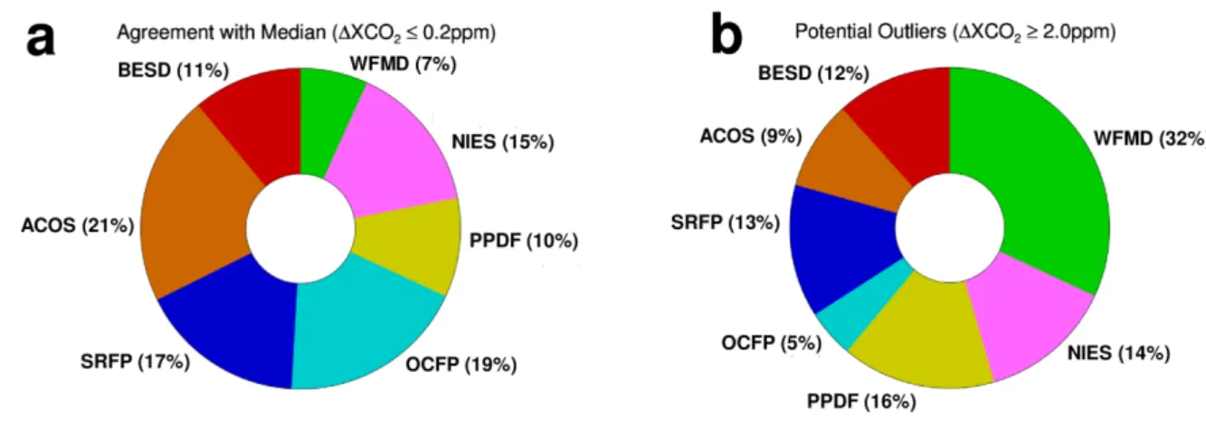
Figures such as Figure 6 also permits the determination of which of the data sets agree and which 602
disagree. For example, the EMMA product, but also most of the individual TANSO products and 603
SCIAMACHY/BESD, agree well or at least reasonably with each other as well as with TCCON and 604
CarbonTracker (see green and yellow smileys), whereas this is not always true for the two very fast 605
algorithms WFMD and PPDF (see red smileys). Figure 7 shows pie charts indicating the overall 606
agreement and disagreement of each of the individual algorithms with the median. The results are 607
consistent with the already reported findings, e.g., better performance of BESD compared to WFMD 608
and similar performance of the TANSO XCO2 algorithms.
609
A large number of other comparisons of the individual data products and the EMMA product with 610
TCCON but also with CarbonTracker have been carried out. Figure 8 shows, as an example, a 611
comparison of the amplitude of the XCO2 seasonal cycle. As can be seen, all satellite data shown
612
suggest that the seasonal cycle is underestimated by CarbonTracker by ~1.5 +/- 0.5 ppm peak-to-peak. 613
Using only a single data product it would be difficult to “prove” that such a relatively small difference 614
24
(~0.3% of the total column) is significant and not caused by or at least significantly influenced by 615
retrieval issues (see, e.g., the discussion given in Schneising et al., 2011, on this topic). Using an 616
ensemble of data products based on more than one satellite and using several essentially independent 617
algorithms allows one to draw more confident conclusions with respect to the interpretation of satellite 618
– model XCO2 differences than would be possible using a single data product only. Within GHG-CCI
619
it is therefore planned to continue the efforts on EMMA in addition to further developing the 620
individual algorithms. 621
5.4 Inter-comparison of SCIAMACHY XCH4 data products
622
The multi-year global retrievals obtained from the two SCIAMACHY XCH4 algorithms, WFMD and
623
IMAP, have been compared with one another. Figure 9 shows, as a typical example, a comparison of 624
one month (August 2005) of the global WFMD and IMAP data products (Figure 10 shows the 625
corresponding results for July 2009; results for other months are shown in Buchwitz et al., 2012a). As 626
can be seen, the monthly XCH4 maps generated with the two algorithms show – depending on region -
627
similar but also significantly different patterns. Both maps show higher methane concentrations over 628
the Northern Hemisphere (NH), where most of the methane sources are located, compared to the 629
Southern Hemisphere (SH). Both data sets agree reasonably well (within typically +/- 10 ppb) over 630
most parts of the SH land areas but over some areas WFMD XCH4 can be up to approximately 20 ppb
631
higher. Over the NH the situation appears to be more complex. Both data sets show elevated methane 632
over large parts of China, south-east Asia and India, but the patterns are not identical, with WFMD 633
being higher over south-east Asia and lower over parts of India compared to IMAP. WFMD and 634
IMAP not only use differently calibrated input data (standard versus non-standard calibration) and 635
different retrieval methods (least squares versus OE), but also different post-processing quality 636
filtering schemes. The latter is reflected by differences in spatial coverage (e.g., WFMD methane is 637
not restricted to land observations only) and number of retrievals over a given region (see right hand 638
side panels of Figure 9). The data density differs significantly depending on region. Typically WFMD 639
has many more data points over the Sahara and other areas in the ~10o-40oN latitude range but also 640
over mid/northern Australia and the mid/western part of the US, whereas IMAP has higher data 641
25
density over South America and mid/high northern latitudes. Large differences between the two data 642
sets are also visible over large parts of northern Africa, where IMAP methane is higher (by approx. 40 643
ppb) and Greenland, where WFMD methane is higher (by approx. 40 ppb). The reasons for the 644
differences have not yet been identified. It has also not yet been assessed to what extent inferred 645
regional methane fluxes would differ depending on which data set is used as input data for inverse 646
modeling of regional methane fluxes. Significant differences can be expected as the regional 647
differences exceed the bias threshold requirement of less than 10 ppb. The discussion also shows that 648
depending on region the differences can be significantly larger than the estimated biases listed in Table 649
5, which are based on the analysis of the satellite data at TCCON sites only. Clearly, more research is 650
needed to understand the differences between the two SCIAMACHY methane data sets discussed in 651
this section. 652
5.5 Inter-comparison of TANSO XCH4 data products
653
Within GHG-CCI, four TANSO XCH4 retrieval algorithms have been further developed and used to
654
generate global data sets which have been inter-compared and compared with TCCON retrievals and 655
global model data (Buchwitz et al., 2012a). The four retrieval algorithms are the FP and PR algorithms 656
developed by SRON (SRFP, SRPR) and Univ. Leicester (UoL; OCFP and OCPR algorithms). 657
For the PR algorithms, which are based on the retrieval of ratios of the CH4 to CO2 columns, followed
658
by a model-based CO2 correction to compute XCH4, the column ratios have been compared as well as
659
the final XCH4 product. As expected, it has been found that the agreement between the ratios is
660
typically somewhat better compared to the XCH4 products due to differences between the model-based
661
CO2 correction as used by SRON and UoL (see Buchwitz et al., 2012a, for details). Overall and in line
662
with the discussion presented in Section 5.2, it has been found that the two PR products agree nearly 663
equally well with the TCCON ground-based observations. A direct comparison of the two data 664
products at TCCON sites is also shown in Figure 11 indicating agreement within typically 10 ppb (1-665
sigma). Nevertheless, inspection of global maps also reveals significant differences, depending on 666
region and time. Qualitatively, this is similar to the results found for the SCIAMACHY data sets 667
discussed in the previous section, but the differences shown in Figure 11 for TANSO are significantly 668