HAL Id: hal-00772180
https://hal.archives-ouvertes.fr/hal-00772180
Submitted on 17 Sep 2020
HAL is a multi-disciplinary open access
archive for the deposit and dissemination of
sci-entific research documents, whether they are
pub-lished or not. The documents may come from
teaching and research institutions in France or
abroad, or from public or private research centers.
L’archive ouverte pluridisciplinaire HAL, est
destinée au dépôt et à la diffusion de documents
scientifiques de niveau recherche, publiés ou non,
émanant des établissements d’enseignement et de
recherche français ou étrangers, des laboratoires
publics ou privés.
Nutrient trapping in the equatorial Pacific: The ocean
circulation solution
Olivier Aumont, James C. Orr, Patrick Monfray, Gurvan Madec, Ernst
Maier-Reimer
To cite this version:
Olivier Aumont, James C. Orr, Patrick Monfray, Gurvan Madec, Ernst Maier-Reimer. Nutrient
trapping in the equatorial Pacific: The ocean circulation solution. Global Biogeochemical Cycles,
American Geophysical Union, 1999, 13, pp.351-369. �10.1029/1998GB900012�. �hal-00772180�
GLOBAL BIOGEOCHEMICAL CYCLES, VOL. 13, NO 2, PAGES 351-369, JUNE 1999
Nutrient trapping in the equatorial Pacific' The ocean
circulation
solution
O. Aumont, J. C. Orr, and P. Monfray
Laboratoire des Sciences du Climat et de l'Environnement, Gif sur Yvette, France
G. Madec
Laboratoire d'Oc6anographie Dynamique et de Climatologie, CNRS/ORSTOM/UPMC
Universit6 Paris VI, Paris, France E. Maier-Reimer
Max Planck Institut flit Meteorologie, Hamburg, Germany
Abstract. Nutrient trapping is a chronic problem found in global carbon cycle models with particle-only remineralization schemes. It is defined as the excess of subsurface nutrient concentrations relative to observations and occurs principally in the eastern equatorial Pacific. Previous studies reduced excess simulated nutrients by increasing the complexity of modeled biogeochemistry, i.e., by adding pools for
nutrients (and carbon) either in dissolved
organic form or as plankton. Conversely,
our study suggests that deficiencies in modeled circulation fields from global coarse- resolution ocean models are mostly responsible. This new interpretation stems
from our use of an ocean general circulation model with higher resolution, which
offers a more realistic equatorial circulation. We used the same biogeochemical
model Hamburg ocean carbon cycle model, version 3, as in some of the previous
studies.
Our model-predicted
distribution
of PO•- in the equatorial
Pacific
agrees
reasonably well with the observations both at the surface and in the subsurface.
Subsurface
PO•- concentrations
in our model's
eastern
equatorial
Pacific
exceed
observations
by, at most, 15%, unlike coarser-resolution
models. Improvement is
due to enhanced meridional resolution (0.5 ø) near the equator, which allows the
model to simulate a vigorous equatorial undercurrent that brings in low-nutrient water from the western basin. Furthermore, the model upwells no nutrient-rich abyssal water into the surface equatorial Pacific. Our results suggest that dissolved organic carbon plays a minor role in the carbon budget of the equatorial Pacific.
1. Introduction
The equatorial Pacific provides the largest source of CO2 from the ocean to the atmosphere. The wind- driven equatorial divergence drives the upwelling of
CO2-rich subsurface water to the surface, thereby in-
ducing
an outgassing
of 0.4-0.9 PgCyr -• [Gammon
et al., 1985; Wong et al., 1993], mostly in the eastern
and central Pacific. The corresponding large subsurface
supply of nutrient maintains intense biological activity,
perhaps representing up to 58% of the global new pro- duction [Chavez and Barber, 1987]. Presumably, the
Copyright 1999 by the American Geophysical Union.
Paper number 1998GB900012.
0886-6236/99/1998GB900012512.00
351
equatorial Pacific's new production could be even higher if the high levels of surface nutrients, abnormal for most
of the ocean, could be used more efficiently. Production appears limited in the equatorial Pacific owing to an in-
sufficient
supply
of iron [Coale et al., 1996]. The equa-
torial Pacific is known for large interannual variability in ocean circulation and air-sea fluxes of CO•. When
upwelling weakens during E1 Nifio-Southern Oscillation
(ENSO) warm events, this source of CO• may almost completely vanish [ Wong et al., 1993].
Global coarse-resolution ocean models coupled to sim-
ple biogeochemical models have been used to improve understanding of the ocean•s carbon cycle [Najjar, 1990;
Bacastow and Maier-Reimer, 1991; Najjar et al., 1992; Maier-Reimer, 1993; Anderson and $armiento, 1995; Yamanaka and Tajika, 1996; Six and Maier-Reimer,
:]52 AUMONT ET AL.: NUTRIENT TRAPPING: A DYNAMIC SOLUTION
ocean general
circulation
models (OGCMs) to repro-
duce the large-scale features of observed tracers such
as •4C, previous
attempt
s have failed when it comes
to
simulating realistic nutrients near the equator with a simple particle-only remineralization scheme. All such forward models have simulated excess nutrient concen-
trations below areas of intense biological production;
model-predicted
nutrients
exceed
obs•?vations
by at
least 50% (1.5 •umolL
-•), particularly
in the eastern
equatorial Pacific [Bacastow and Maier-Reimer, 1990;
Najjar et al., 1992;
Maier-Reimer,
1993; Yamanaka
and
Tajika, 1997]. This flaw, termed "nutrient
trapping"
by Najjar [1990],
results
from a positive
feedback
be-
tween intense production induced by the upwelling of nutrient-rich abyssal waters and remineralization of or- ganic matter within the divergence.
To remedy this model artifact, efforts have focused on apparent oversimplifications in modeled biogeochem- istry. The first proposed biogeochemical remedy for nu- trient trapping was motivated by new measurements of surprisingly large concentrations of dissolved organic
carbon
(DOC) [Suzuki
et al., 1985;
$ugimura
and Suzuki,
1988]. Ocean
modelers
who added a large, long-lived
DOC pool to their particle-only models did indeed find substantial reduction in nutrient trapping [Najjar,
1990; Bacastow
and Maier-Reimer, 1990; Najjar et al.,
1992; Anderson
and $armiento, 1995]. Adding a DOC
pool decreases the amount of nutrients exported to
depth by particles. Because
it is long lived, much of
the DOC is exported laterally away from the problem- atic equatorial Pacific. Analytical problems were even-
tually shown
to be the cause
of the high measured
DOC
[Suzuki,
1993]. Modelers
had to find another
solution
to the nutrient-trapping artifact.
Six and Maier-Reimer [1996] have proposed
a sec-
ond solution to nutrient trapping. They have also sug-
gested
that an oversimplified
ocean biogeochemistry
is
to blame. To improve matters, their new biogeochemi-
cal model includes interactions between phytoplankton and zooplankton, as well as a reservoir of semilabile DOC having a much shorter lifetime than that used
previously. As a result, in the eastern equatorial Pacific
Ocean, the presence of a large standing stock of zoo-
plankton reduces primary production and resulting ex- port production. Additionally, a significant part of the
organic matter is exported laterally as DOC away from the divergence. Combination of both factors (zooplank- ton grazing and horizontal DOC transport) reduces ac-
cumulation of nutrient below the divergence.
Another possibility, that faulty model circulation fields
may cause nutrient trapping has not been explored pre-
viously with simulations in OGCMs, which, by defini- tion, predict a three dimensional (3-D) ocean circula- tion field. However, Matear and Holloway [1995] sug- gest that the OGCM circulation fields may be partly
to blame. Simulated subsurface nutrient concentra-
tions in their adjoint model become more realistic when they stipulate that the 10 Sv upwelling in their origi- nal advection field, taken from the Hamburg large-scale
geostrophic (LSG) model [Maier-Reimer et al., 1993],
is replaced by downwelling. That coarse-resolution models overpredict equatorial upwelling has been sug-
gested for some time [Toggweiler et al., 1991]. Although Matear and Holloway [1995] seem to have identified one
potential problem, more refined OGCM's are needed to determine the causes of this and other circulation defi- ciencies, which may contribute to nutrient trapping.
With such in mind, we have compared simulations from two very different OGCMs that have both used one common biogeochemistry. For our study, we implanted
the Hamburg ocean carbon cycle model (HAMOCC3) developed by Maier-Reimer [1993] in OPA (Ocean Par-
all•lis•), an ocean general circulation model developed at the Laboratoire d'Oc•anographie Dynamique et de Climatologie (LODYC) in Paris. Then we compared our results to those obtained previously, with runs of
HAMOCC3 in the LSG model from Maier-Reimer [1993].
We found that the OPA-HAMOCC3 model produces little nutrient trapping (model predictions exceed ob-
served
PO4
•- by 15%, at most);
the LSG-HAMOCC3
combination [Maier-Reimer, 1993] produces larger ex- cesses (up to 100%). In the equatorial Pacific, OPA's
high resolution and its prognostic parameterization of vertical turbulence provide circulation fields that are more realistic. Critical features exhibited by OPA, but
not by other coarse-resolution global OGCMs, include
(1) little upwelling of deep water to the surface and (2) a
strong and narrow equatorial undercurrent. To demon- strate how the artifact of nutrient trapping is sensitive to model resolution, we present results from a sensitivity test that varied the horizontal eddy viscosity coefficient.
2. Model Description
In this study, the ocean's preindustrial state is simu-
lated by implanting HAMOCC3 [Maier-Reimer, 1993]
into a tracer-transport model driven by 3-D advective and diffusive fields predicted by the OGCM known as
OPA [Delecluse et al., 1993]. Here we outline the im-
portant aspects of both the physical and biogeochemical models.
2.1. Ocean General Circulation Model
The OGCM used here was first developed a decade
ago [Andrich, 1988]. Known as OPA, it has been mod- ified for use as a regional [Blanke and Delecluse, 1993; Maes et al., 1997] and global-scale model [Marti, 1992;
Delecluse et al., 1993; Madec and Imbard, 1996; Guil-
yardi and Madec, 1997]. OPA solves the primitive equa- tions discretized on a C grid [Arakawa and Lamb, 1977]
using the classical Boussinesq and rigid lid approxima-
AUMONT ET AL.- NUTRIENT TRAPPING- A DYNAMIC SOLUTION 353
onal, which ensures a second-order numerical accuracy
[Marti et al., 1992]. The grid is distorted in the northern
hemisphere so that the northern singularity is shifted to be over Asia. Horizontal grid spacing varies between 0.5 ø and 2 ø with its higher meridional resolution in the
equatorial regions as a means to better resolve fine-
scale features important in equatorial dynamics. The model has 30 vertical levels, among which 10 are lo- cated in the top 100 m. The model is driven with the
monthly
mean
climatology
of wind stress
[Hellerman
and Rosenstein, 1983]. Heat fluxes and water fluxes are from Oberhiiber [1988]. Additionally, temperature
T and salinity $ are restored at the surface toward cli-
matological values [Levitus, 1982] using a damping time
constant of 12 days.
Effects of nonresolved subgrid-scale movements on
the large-scale circulation are parameterized by horizon-
tal and vertical eddy diffusivities and viscosities. The horizontal eddy viscosity coefficient is imposed by the
resolution. It is set to be equal to 4x10⁴ m 2 s -1 ev-
erywhere, except between 20øS and, 20øN, where it is
gradually
reduced
to attain 2000 m 2 s -1 at the equa-
tor. This reduction accounts for the ratio between the
typical scale of the eddies and the horizontal spacing, which is smaller when near the equator than in higher latitudes. The horizontal eddy diffusivity coefficient is
constant
everywhere
at 2000 m 2 s -•. Vertical eddy dif-
fusivity is not defined a priori. Instead, OPA includes a
prognostic model of the turbulence based on the equa-
tions of the turbulent kinetic energj• (TKE) model pro- posed by Gaspar et al. [1990] and adapted to OPA by Blanke and Delecluse [1993]. Thus OPA predicts turbu-
lence and computes vertical eddy diffusivity and viscos-
ity coefficients throughout the water column, i.e., within
the mixed layer as well as below.
Because of OPA's relatively high horizontal and verti-
cal resolution, it is run in a semidiagnostic mode; T and
$ are restored toward the climatological values of Levi-
tus [1982] not only at the surface (where this restoration •s part of the boundary conditions) but also through-
out most of the ocean. The restoring time constant
used varies with depth from 50 days at 15 m (level 2 of OPA) to 1 year in the deep ocean. This approach
is conceptually similar to the technique used by Togg-
weiler et al. [1989] in their "robust-diagnostic" version of the Geophysical Fluid Dynamics Laboratory (GFDL)
model. Practically, though, there are major differences. In OPA, T and $ are always restored in the first level,
but below that, restoration is relaxed in four areas: (1)
in the mixed layer, which is thus predicted prognosti-
cally, (2) in the equatorial regions, where small errors
in observed density would lead to large errors in model-
predicted velocity fields [Fufio and Imasato, 19911, (3)
in the high latitudes, where measurements are rare and
biased toward summer values, and (4) along ocean-land
boundaries to allow the model to reconstruct its own boundary currents.
Here we have used a tracer-transport (offiine) ver- sion of OPA developed by Marti [1992]. This model
uses monthly mean fields of advection, turbulence, T, and $, as predicted by the on-line model. Advective
transport of tracers is computed according to the MP-
DATA scheme of $molarkiewicz [1982, 1983], and $mo- larkiewicz and Clark [1986]. Although expensive, this scheme is little diffusive and positive definite (that is, it avoids negative tracer concentrations).
2.2. Carbon-Cycle Model
The biogeochemical model HAMOCC3 [Maier-Reimer
1993] is coupled to OPA. Our first priority was to keep
HAMOCC3 in its original state in order to allow a rigor- ous comparison of our results with results from Maier-
Reimer [1993]. Although some minor adaptations were
necessary, their effect is negligible as discussed below.
We have made three changes in HAMOCC3 when we implemented it in OPA. First, the number of the sim- ulated tracers has been reduced to 7 instead of the 20 included in the original model. This change was performed in order to reduce the computing cost of
the combined OPA-HAMOCC3 model. Second, we
computed the piston velocity using the formulation
from Wanninkhof [1992] instead of using a constant value as in the work by Maier-Reimer [1993]. How- ever, changes in the piston velocity do not affect the
predicted distribution of phosphate. Third, we did not
keep HAMOCC3's simple sedimentation model in OPA
because a much longer integration would be necessary
to equilibrate the model (tens of thousands of years in- stead of several thousand years).
For more efficient use, we included only the seven
prognostic tracers necessary for the computation of the
different biogenic fluxes of carbon: dissolved inorganic
carbon
(DIC), alkalinity,
02, calcite,
PO•-, particulate
organic carbon (POC), and dissolved silicate. These
fluxes are divided into two components; the soft tissue
pump and the hard tissue counterpump. The soft tissue pump is reduced, in the model, to the export produc-
tion (EP), defined simply as the part of the primary
production transported out of the euphotic zone. EP is computed as
EP_r015__0
Zm T + 10 [eo•-] + P0
T+2
([PO•-])[PO•-]
(1)
where r0 is the maximum productivity rate, I is a nor-
malized light factor, Zm is the mixed layer depth, T is temperature (degrees Celsius), and P0 equals 0.02
/•mol P L -•. Export production
in nutrient-poor
water
is reduced by a simple Michaelis-Menten kinetics for-
354 AUMONT ET AL.' NUTRIENT TRAPPING: A DYNAMIC SOLUTION
[Dugdale,
1967].
In HAMOCC3,
PO•- is chosen
as the
limiting nutrient to avoid complexities associated with nitrogen cycling. The thickness of the euphotic zone is set to 50 m globally. The light factor I is defined as the integration of the cosine of the solar angle over the day length, normalized to be comprised between 0 and 1. Cloud cover is ignored in this computation. The max-
imum production efficiency r0 is set to 0.25/month as chosen by Maier-Reimer [1993] to adjust his model out-
put to fit the observed surface phosphate distribution. The significance of the chosen value for r0 is that, at
most,
25% of local
PO4
•- can be removed
each
month
from the surface by biological activity. The intensity of the hard tissue counterpump is deduced from export
production via the rain ratio (organic C/CaCO3 ratio) [Broecker and Peng, 1982]. This ratio depends on T and the local concentration of dissolved silicate. The maximum value of the rain ratio is set in HAMOCC3
to 0.35.
POC produced in the euphotic zone is exported in-
stantaneously below 100 m. The vertical profi!e of the
POC flux is described according to a power law function
z -ø's [Berger
et al., 1987]. In HAMOCC3, denitrifica-
tion is not considered. Thus the remineralization of the organic matter is restricted to regions with sufficient
oxygen
(>_ I/•mol L -1 ). Otherwise,
POC is preserved
and transported by advection and diffusion.
At the sea surface, the ocean exchanges CO2 and 02
with the atmosphere. The net flux from air to sea F is proportional to the difference between the partial pres- sure of the gas in air Pa and that in surface seawater p,.
F - ka(P• - P,) (2)
where k is the gas transfer velocity (in ms-l), c• is
the gas solubility
(mot
m -3 •uatm
-1). Instead of using
a constant coefficient as did Maier-Reimer [1993], we
computed the piston velocity of CO2 by using equa-
tion (8) from Wanninkhof [1992], a quadratic function
of wind speed that includes a chemical enhancement at low wind speeds. We used a climatology of the
monthly mean wind speeds and variances [Boutin and Etcheto, 1997] derived from special sensor microwave images (SSM/I) wind speeds [Wentz, 1002]. The re- sulting gas exchange coefficient K (K - ks) for CO2
has been
scaled
so that its gtobai
mean
value
equals
0.061 mot m -2 •uatm
-1 yr -1 deduced
from 14C observa-
tions [Broecker et al., 1985]. The piston velocity of 02
is is computed according to the formulation from Liss
and Merlivat [1986].
Besides the numoer of b•ogeoc,,em•cm •' ' • ' • tracers and the formulation of the piston velocity, we made a third change in HAMOCC3. The simple parameterization of
the sedimentation processes was eliminated because the
long timescales associated with the sediments, on aver-
age, 45,000 years [Maier-Reimer, 1993], require very
long model integrations that were beyond our means. However, fluxes between the ocean and the sediments as predicted by the original version of HAMOCC3 cou- pled to the LSG model are quite small, particularly for
organic matter [Maier-Reimer, 1993]. Omitting these
fluxes should not significantly alter modeled tracer dis- tributions, especially that of phosphate in the upper equatorial Pacific Ocean.
2.3. Initial Conditions and Model Integration Simulations are initialized with uniform distributions
of tracers.
PO43-
concentration
is set to 2.1 /•molL
-1
, the observed global mean computed from Conkright
et al. [1994]. Dissolved inorganic carbon is set to be 2350/•mol L -1 . Total alkalinity is initialized to 2374
/•eqkg
-1 [Takahashi
et al., 1981]. Preindustrial
atmo-
spheric pCO2 is fixed at 278 ppm.
True steady state is reached when the globally and
annually averaged air-to-sea flux of CO2 is zero. Since,
in theory, this would require an infinitely long integra-
tion, we chose
a small threshold
value (0.05 PgC yr-1),
below which the model was considered to be at equilib- rium. To speed simulations, we used our recently devel-
oped technique,
DEGINT [Aumont
et al., 1998], which
accelerated off-line simulations described here by a fac-
tor of 20. At equilibrium, the model's annual mean air-
to-sea COe flux, integrated globally, is 0.05 PgC yr -1.
3. Results
3.1. Simulated Equatorial Pacific Dynamics
Intense currents of limited meridional extent char-
acterize equatorial dynamics in the Pacific. OPA's en-
hanced meridional resolution in this region improves the
equatorial dynamics relative to other coarse-resolution
global models. Below we discuss the main dynamic fea- tures of OPA that play a role in controlling the distri-
bution of the biogeochemical tracers.
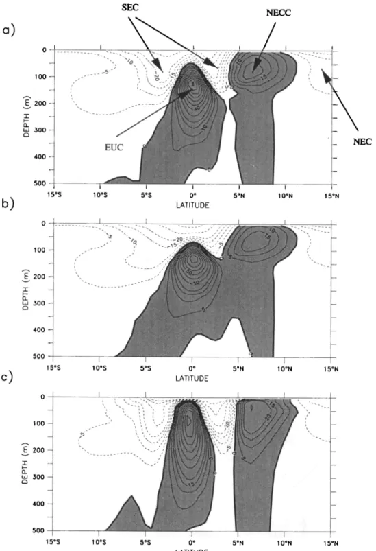
Figure I shows a section of the zonal velocity field
along 150øW. , This section reveals that equatorial cur-
rents in OPA compare reasonably well with the observa-
tions of Wyrtki and Kilonsky [1984]. In particular, OPA
is able to simulate a vigorous equatorial undercurrent
(EUC) centered at the equator, whose speed exceeds
I ms -1. The model maximum
speed
of 1.4 ms -1 at
140øW
is close
to that observed
(1.6 m s -i) [Qiao and
Weisberg,
1997]. Below
the EUC, observations
[Wyrtki
and Kilonsky, 1984] show the presence of a geostrophic
westward current, the equatorial intermediate current
(EIC), whose speed can reach 0.15 ms -1. The model
does not clearly reproduce the EIC. However, we know of no model that is able to reproduce such a current on an annual mean. OPA simulates a stronger EIC dur-
ing boreal summer. In August, simulated speeds reach
AUMONT ET AL.: NUTRIENT TRAPPING: A DYNAMIC SOLUTION 355
SEC
NECC
,..
,:
,,
'200
'
'
'
•00400
500 100 •200 •00 400 500 15øS 10øS 5øS 0 ø 5øN 10øN 15øNC )
LATITUDE
100 - 200- 300- 400 -- 500 15øS I 1 I I 10øS 5øS 0 o 5ON 10øN 15øN I ATITt Jl-)FFigure 1. Annual mean distribution of zonal velocities (cms -x) simulated by the Ocean Par- all•lis• model (OPA) along 150øW in the near surface for (a) the standard simulation, (b) case
HV, and (c) case CVD. Positive speeds indicate eastward flow.
which, incidentally, is of roughly the same magnitude
as that offered by Wyrtki and Kilonsky [1984] as the annual mean.
At the surface, the south equatorial current (SEC),
flowing westward, exhibits two distinct maxima, one
north and one south of the equator (Figure 1). The SEC's double maximum is due to frictional effects of
the EUC, which flows in the opposite direction and splits the SEC below the surface. The SEC is limited to the upper 200 m and is more rapid in the north.
AUMONT ET AL.: NUTRIENT TRAPPING- A DYNAMIC SOLUTION 357 5' N
-•
E
q
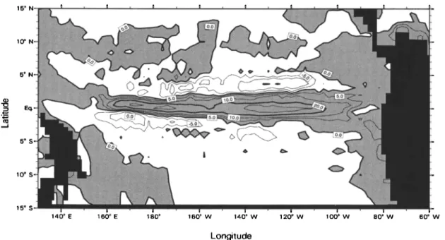
5 ø S 10 ø S 15 ø S 140 ø E 160 ø E 180 ø 160 ø W 140 ø W 120 ø W 100 ø W 80 ø W 60 ø W LongitudeFigure 3. Modeled
annual
mean
vertical
velocities
(in 10
-6 ms -•) in the equatorial
Pacific
at
50 m. Contour levels are drawn at 0, 5, 10, 20, and 30x10 -6 ms -•.
The associated vertical transport equals 38.6 Sv at 50
m for the area within 170øE to 100øW and 5øS to 5øN. Observed values range from 37 to 51 Sv [Wyrtki, 1981].
The equatorial divergence in OPA exhibits large sea-
sonal variability with distinct maxima in April-May and October-November, as in the observations [Poulain, 1993]. Along the Peruvian coast, northward wind stress
forces coastal upwelling between 2øS and 15øS. In this
area, OPA transports 3.8 Sv upward toward the surface
in agreement
with the observed
4 Sv [Wyrtki, 1963].
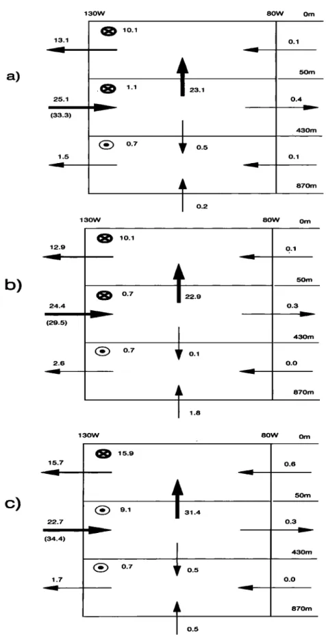
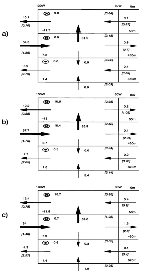
To help diagnose tracer distributions in the equato-
rial Pacific, we determined the model's annual mean
water transport budget for the upper eastern Pacific Ocean (Figure 4a). This region is exactly where coarse- resolution models develop nutrient trapping [Najjar et al., 1992; Maier-Reimer, 1993]. Laterally, the region is de- fined as that between 130øW and 80øW and between
5øS and 5øN. Vertically, we further divided this region
into three zones' (1) the surface euphotic zone located in the top 50 m; (2) the intermediate zone between 50 and 423 m, which is affected by the EUC; and (3) the deep zone (423-870 m), where nutrient trapping is at
its maximum. The equatorial divergence upwells 23.1
Sv of middepth waters into the productive surface zone.
More than half of that is transported westward by the SEC out of the region defined above; the rest escapes meridionnally.
The divergence is fed by water from the core of the
__
EUC, which
itself
advects
33.3 Sv into the
' domain.
The
water flux at 130øW is substantially less (25.1 Sv) be-
cause in that region, the middepth box also includes the
lower part of the westward flowing SEC. At 80øW, the
EUC nearly vanishes owing to continuous upwelling and
subsequent poleward divergence near the surface. The
meridional geostrophic loss of water is small (1.1 Sv).
Across the EUC, there is no input of water from the deep ocean. The deepest box correspond to the domain that should be affected by the EIC. Associated trans- port is 1.5 Sv, about I order of magnitude too small relative to annual mean estimates of Wyrtki and Kilo-
nsky [1984].
3.2. Simulated
PO43-
Figure 5 shows the annually averaged distribution of
surface
PO43-
as taken from the top 5 m in the Na-
tional Oceanographic Data Center (NODC) world at- las [Conkright et al., 1994] and the top 10 m simulated
by OPA. Maximum
simulated
PO43-
concentrations
are
found in the Peruvian upwelling, where they exceed 1
pmolL -•, in agreement with observations. Upwelled
waters are transported northward and westward. Ow- ing to the westward transport both in the model and observations, the Peruvian upwelling appears to feed
the divergence
with substantial
PO43-
. However,
it re-
quires about 10 months for the water to move from the Peruvian coast to where the divergence is at its maxi-
mum (120øW), as determined from the modeled zonal velocity of 10 cm s -• in this region. Thus most of the
upwelled
PO43-
is consumed
in the model
by biota be-
fore it reaches the divergence, because in that region modeled production efficiency is close to its maximum
AUMONT ET AL.- NUTRIENT TRAPPING: A DYNAMIC SOLUTION 357
1
1
140 ø E 160 ø E 180 ø 160 ø W 140 ø W 120 ø W 100 ø W 80 ø W 60 ø W
Longitude
Figure 3. Modeled
annual
mean vertical
velocities
(in 10
-6 ms -1) in the equatorial
Pacific
at
50 m. Contour levels are drawn at 0, 5, 10, 20, and 30x 10 -6 ms -1.
The associated vertical transport equals 38.6 Sv at 50
rn for the area within 170øE to 100øW and 5øS to 5øN. Observed values range from 37 to 51 Sv [Wyrtki, 1981].
The equatorial divergence in OPA exhibits large sea-
sonal variability with distinct maxima in April-May and October-November, as in the observations [Poulain, 1993]. Along the Peruvian coast, northward wind stress
forces coastal upwelling between 2øS and 15øS. In this area, OPA transports 3.8 Sv upward toward the surface
in agreement
with the observed
4 Sv [Wyrtki, 1963].
To help diagnose tracer distributions in the equato- rial Pacific, we determined the model's annual mean
water transport budget for the upper eastern Pacific Ocean (Figure 4a). This region is exactly where coarse- resolution models develop nutrient trapping [Najjar et al., 1992; Maier-Reimer, 1993]. Laterally, the region is de- fined as that between 130øW and 80øW and between
5øS and 5øN. Vertically, we further divided this region
into three zones: (1) the surface euphotic zone located in the top 50 m; (2) the intermediate zone between 50 and 423 m, which is affected by the EUC; and (3) the deep zone (423-870 m), where nutrient trapping is at
its maximum. The equatorial divergence upwells 23.1
Sv of middepth waters into the productive surface zone.
More than half of that is transported westward by the SEC out of the region defined above; the rest escapes meridionnally.
The divergence is fed by water from the core of the
EUC, which
itself
advects
33.3
Sv into the domain.
The
water flux at 130øW is substantially less (25.1 Sv) be-
cause in that region, the middepth box also includes the
lower part of the westward flowing SEC. At 80øW, the
EUC nearly vanishes owing to continuous upwelling and
subsequent poleward divergence near the surface. The
meridional geostrophic loss of water is small (1.1 Sv).
Across the EUC, there is no input of water from the deep ocean. The deepest box correspond to the domain that should be affected by the EIC. Associated trans- port is 1.5 Sv, about I order of magnitude too small relative to annual mean estimates of Wyrtki and Kilo-
nsky [1984].
3.2. Simulated
PO4
•-
Figure 5 shows the annually averaged distribution of
surface
PO4
•- as taken from the top 5 rn in the Na-
tional Oceanographic Data Center (NODC) world at-
las [Conkright et al., 1994] and the top 10 rn simulated
by OPA. Maximum
simulated
PO•- concentrations
are
found in the Peruvian upwelling, where they exceed 1
•umolL -1, in agreement with observations. Upwelled
waters are transported northward and westward. Ow- ing to the westward transport both in the model and observations, the Peruvian upwelling appears to feed
the divergence
with substantial
PO4
•- . However,
it re-
quires about 10 months for the water to move from the Peruvian coast to where the divergence is at its maxi-
mum (120øW), as determined from the modeled zonal velocity of 10 cms -1 in this region. Thus most of the
upwelled
PO4
•- is consumed
in the model
by biota be-
fore it reaches the divergence, because in that region modeled production efficiency is close to its maximum
358 AUMONT ET AL.' NUTRIENT TRAPPING: A DYNAMIC SOLUTION a)
b)
13.1 25.1 (33.3) 1.5 12.9 24.4 (29.5) 2.6 130W 80W Om 10.1 0.7 130Wt23.1
0.5 0.1 50m 0.4 430m 0.1 870m 0.2 80W Om 10.1 0.7 0.7t22.9
0.1 50m 0.3 430m 0.0 870m 130W 80W Omc)
15.7 22.7 (34.4) 1.7 15.9 0.7 31.40.5
0.5
0.6 50m 0.3 430m 0.0 870mFigure 4. Water mass budget in the upper eastern equatorial Pacific Ocean for (a) the standard simulation in OPA, (b) case HV, and (c) case CVD. Region limits are 80øW-130øW, 4.7øS -
4.7øN, and 0-870 m. Circled crosses indicate transport out of the domain; circled dots represent
transport into the domain. Numbers in parentheses denote the transport associated with the
AUMONT ET AL.- NUTRIENT TRAPPING: A DYNAMIC SOLUTION 359 15 ø
a)
5 • N 5 • S' 10øS- 15•S -120øE 140øE 160øE 180 ø 160øW 140øW 120øW 100øW 80*W 60øW
b)
Longitude15ø
I v ' I , I , I , I I / , I [ I ,
10 •,5
ø
N
'
(•
E 120 ø E 140 ø E 160 ø E 180 ø 160 • W 140 ø W 120 ø W 100 ø W 80 ø W 60 ø1W LongitudeFigure 5. Annual
mean
distribution
of PO4
•- (•umol
L -1 ) at the sea
surface
in the equatorial
Pacific,
showing
(a) observations
from Conkright
et al. [1994]
and (b) output from OPA. Contours
are given
for every
0.1 •umol
L -1 .
105øW, the model simulates a second maximum. Also located there is the model's local maximum in vertical velocity.
Both modeled
and observed
distributions
of PO4
•-
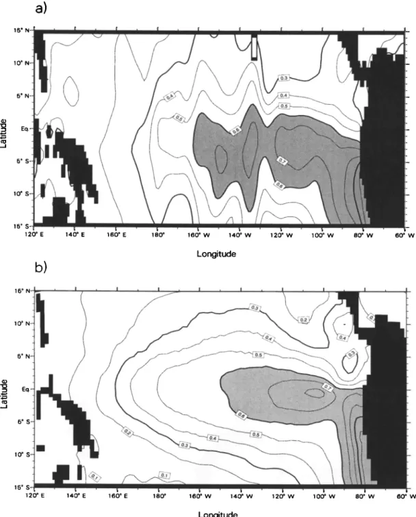
are asymmetrical with respect to the equator. East of 150øW, maximum surface concentrations are located mainly in the southern hemisphere. Lower values in
the northern hemisphere, noticed previously for nitrate
[Toggw½iler ½t al., 1991], are due to the NECC, which
brings in waters with lower nutrient concentrations from
the western
Pacific
[Toggweiler
and Carson,
1995].
Figure
6 shows
sections
of observed
PO4
•- and mod-
eled total phosphorus concentrations along the equator
in the Pacific ocean. In the model, we consider total
phosphorus
(PO4•-+POP)
because
the model's
lack of
oxygen in the eastern Pacific ocean produces a large pool of unreminoralized POC [Maier-Reimer, 1993, Fig- ures 14a and 14b]. Total P can be defined as that P
:]60 AUMONT ET AL.: NUTRIENT TRAPPING: A DYNAMIC SOLUTION a) loo 0.4. 0.6 300 ;- ... i•,•>.::..::• z•,. •:' •:• •:,'•:• 300 •-•.' ..a:.•- -•:•:./•• ß ..,' . .•:•.:-•:•:.:•:<•:•,• - ... ?;'•{. •:• .•:•;•:-:'•
ß
, :•.
z.4
'•'•--•,•%•••-•/•,.--
•/••
--'2•.-•
....
'• ....
-,•.•'-•
...
125" S 150" S 175" S 160" W 135" W 11• W 85" W 60" W b) LONGITUDE o 1-.6•100
•
0.4 06
•
0.8
0.8
0.B
200 10 1.0 _ ' - - ' • • • 2.•-• •'•"• •oo • ß - •. ,.,.•:•'•-: • - ,- .•:..•:•:..:•..:½•.::.:....;.•:m:::::: •,. ,•:• ... r-. ... • .... • B •' .•:•.- ... • •:: .:•: .:<:< ::•---½.... ... • ........
'
".<-:< ....
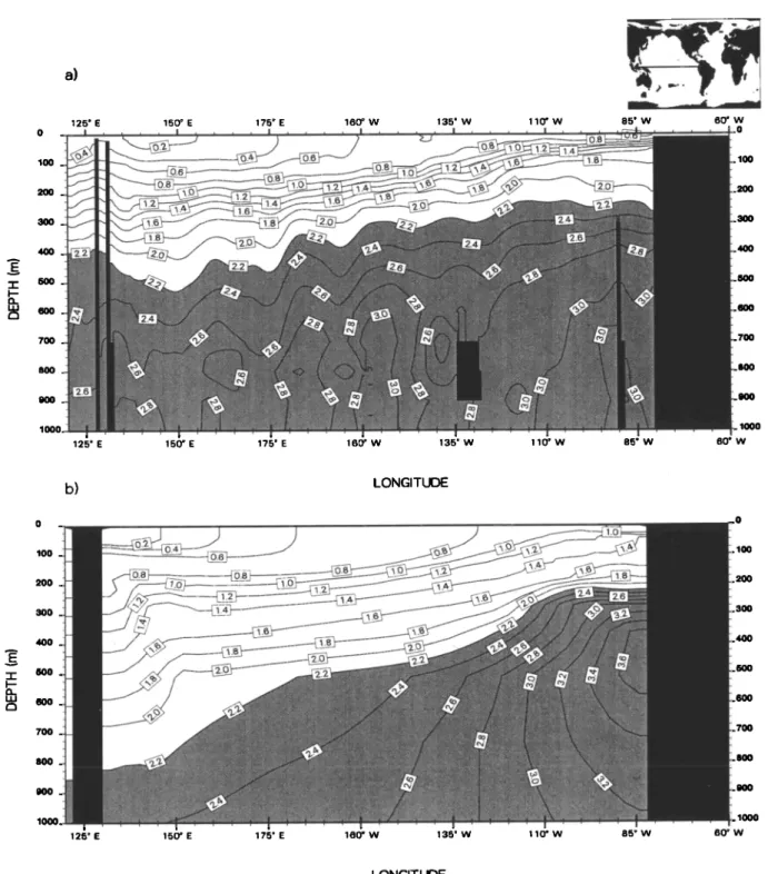
,•:- ,- ,... ,•.:•/• ... ..•..< : •:•. • •:. ,. .. , . :• ... :•' .+•:. . , < .... : ... --... :::: : :•::j,..•: :• :•'" -a. '-•:' . .. :'::":• ' ,4: :,-- .. :-:': ... ., ========================== 125 ø E 150 ø E 175 ø E 160 ø W 135 ø W 110 ø W 85 ø W lOO 200 300 4OO 5OO 6OO 700 8OO 8OO lOOO 60" w LONGITUDEFigure õ. Annual
mean
distribution
of PO4
•- (/•molL
-1 ) in the upper
1000m
of the water
column along the equator in the Pacific, showing (a) observations from Conkright et al. [1994], (b) standard case, (c) case HV, and (d) case CVD. For the model, total phosphorus is considered
instead
of PO4
•- alone,
as explained
in the text. Black
areas
in Figure
6a correspond
to the
bathymetry but also to regions where data are unavailable.
which is potentially available for biological consump- tion. To infer the sensitivity of the total P distribu-
tion to this lack of oxygen, we made a test (not shown) with the model where remineralization occurs even af- ter waters become anoxic. The total P distribution is
nearly unchanged. Considering previous modeling ef-
forts, it is remarkable that OPA-HAMOCC3 exhibits
only a minor case of nutrient trapping. At 800 m,
the model's maximum concentration
is 3.4 /•molL -1
, about 0.4 /•mol L -1 higher than in the obervations.
AUMONT ET AL.- NUTRIENT TRAPPING: A DYNAMIC SOLUTION 361 lOO 200 300 400 500 600 700 800 900 lOO 200 300 400 500 600 700 800 900 1000 c) 1.0
12õøE Iõ0øE 17õ•E 160øW 13õøW 110øW 8õøW LONGITUDE
d)
12õøE IõO;E 17õ•E 160•W 13õøW 110=W
,100 200 400 500 700 800 900 lOOO w lOO .200 300 500 600 700 800 900 lOOO 6o • w LONGITUDE Figure 6. (continued)
In comparison, the difference between modeled and ob-
served concentrations exceeds 2.5/•mol L -z in the work
of Maier-Reimer
[1993]
and 1.5/•mol
L -1 in the work of
Najjar et al. [1992] at about the same depth. Since we
use the same biogeochemical model as MaieroReimer
[1993], the improvement must be due to the different
modeled circulation, particularly the different equato-
rial dynamics. Causes of the improvement are examined below.
On its way eastward, the EUC is progressively en-
riched
in PO4
•- owing
to export
production
from
above.
Originating in the far western Pacific Ocean, the EUC
advects
water
having
lower
PO4
•- concentrations
into
waters
enriched
in PO4
•- . Thus
the EUC dilutes
mid-
362 AUMONT ET AL.: NUTRIENT TRAPPING: A DYNAMIC SOLUTION
depth waters that are brought to the surface by the di-
vergence. As a consequence, the undercurrent is largely
responsible for the sharp vertical gradient between 50 and 400 m. The model's vertical gradient is weaker than observed, in part because the simulated EUC ex- tends too deeply; that is, there is no EIC (see section
3.1). The model's poorly constrained remineralization
scheme may also be somewhat responsible.
3.3. PO43-
Budget
To better understand why OPA exhibits little nu- trient trapping, we constructed a phosphorus budget for the eastern equatorial Pacific (Figure 7a), divid- ing the region into the same three vertical layers as
for the water mass budget (Figure 4). The EUC's
role in this budget seems a paradox, as noted by Tog-
gweiler and Carson [1995]. On one hand, the EUC is
the major supplier of water and nutrients, advecting
34.3 kmo! P s -1 into the upwelling system; on the other hand, the EUC dilutes nutrient concentrations of the
waters upwelled toward the surface because its source
is in the west,
where
PO43-
concentrations
are, on aver-
age, 0.6 pmol L -1 lower than in the intermediate zone
of the eastern equatorial Pacific.
Of the 42.1 kmolPs -1 brought into the interme-
diate box by the EUC and export production from
above,
three fourths (31.5 kmol P s -1) is upwelled
into
the productive zone. The.remaining one fourth (8.9
kmol P s -1) is advected
latitudinally;
75% of that is lost
by transport to the south. Some of this southward out- flow eventually feeds into the Peru upwelling. Such is consistent with observations that indicate that waters upwelled off the coast of Peru originate from the lower
part of the EUC [Wyrtki, 1963; Lukas, 1986; Toggweiler et al., 1991].
In the euphotic
zone,
about 2/3 (19.9 kmolP s -1) of
the PO43-
upwelled
from
the midlayer
box
exits
the sur-
face box laterally. Lateral loss is divided nearly equally between transport by the westward flowing SEC and meridional transport across the southern and northern
edges. Toggweiler and Carson [1995] found a some-
what lower amount, about 50%, leaving the surface box by lateral export, after summing transport of ni-
trate (30%) and organic matter (20%). Concerning the
remaining
one third (11.7 kmolP s -1) of the phospho-
rus that leaves the euphotic zone in OPA-HAMOCC3, it is exported into deeper layers by sinking particles. The mean POC export rate was estimated to be 3
mmol
C m -2 d -1 by Murray et al. [1994]
at 120 m along
140øW,
using
the 234Th
method
[Buesse!er
eta!., 1992].
At the same depth and location, the modeled export
production
is 6.6 mmol
C m -2 d -1, which is more than
2 times higher. However, fluxes of organic matter in this region exhibit a large temporal variability, and •tata-based estimates are relatively uncertain. POC
export estimates at the same location can be signifi-
cantly higher according to Murray et al. [1996], who used information from both 234Th and drifting sedi-
ment traps. Their export estimates range from 2 and
30 mmol C m -2 d -1 during September 1992, a period characteristic of non-E1 Nifio conditions.
Fluxes into and out of the deep box are much smaller. In OPA, there is little input of phosphorus from the deep ocean. None of that makes it across OPA's strong EUC. Such minimal upwelling is remarkable for coarse- resolution global models but not for high-resolution re-
gional
models
[Toggweiler
and Carson,
1995]. This lack
of upwelled deep phosphorus was expected in view of
the water mass budget. Phosphorus entering the deep
box by transport or export production leaves it through the deep box's western limit.
Observational and modeling studies [Tsuchiya, 1981; Toggweiler et al., 1991; Blanke and Raynaud, 1997] have
shown that most of the water entering into the equato- rial Pacific's source zone for the EUC derives from the southern hemisphere. To better determine its source in
OPA, we analyzed
nutrient t•ansport in the area be-
tween 5øS and 5øN and 130øE and 150øE (not shown), where the EUC originates. We found that of the 16
kmol P entering that box every second, roughly 70% de-
rives from the southern hemisphere, mostly transported
by the New Guinea Undercurrent (NGUC).
3.4. Sensitivity Tests
O PA has two peculiarities that have the potential to contribute to its improved ability to match observed phosphate. First, OPA's 0.5 ø meridional resolution near the equator is enhanced relative to the roughly 4 ø resolution used by other global-scale, coarse-resolution models. Second is OPA's prognostic parameterization
of vertical turbulence (TKE) throughout the water col-
umn. OPA's semidiagnostic forcing is unimportant here
because OPA is completely prognostic in the equatorial
region. The combination of higher resolution and the TKE model of vertical turbulence are together respon- sible for the absence of substantial nutrient trapping in OPA. To determine the contribution of each factor, we performed two sensitivity tests with the on-line version
of OPA (Table 1).
For the first test, we increased the equatorial hori-
zontal viscosity
coefficients
used
in OPA (2000 m 2 s -i)
by a factor of 20 to their extratropical value (40,000
m 2 s -1). We term this as case
HV. Such
an experiment
is motivated by the use of large horizontal eddy viscosity coefficients in coarse-resolution models, as required to
avoid numerical problems (i.e., to simulate smooth solu-
tions). Owing to such high viscosity, simulated horizon-
tal speeds in coarse-resolution models are often underes-
timated, particularly the speed of the EUC [Toggweiler et al., 1989]. However, our case HV is not exactly equiv-
AUMONT ET AL' NUTRIENT TRAPPING' A DYNAMIC SOLUTION 363
a)
b)
10.1 [0. 76] 34.3 [1.56] 3.9 [2. 73] 12.2 [0.88] 37.7 [1.75] 7.7 [2.85] •OW 80W Om 9.8 [0.84] -11.7 (•) 8.9 7.8 • 0.6 31.5 [2.18] 1.4 0.9 0.1 [0.87] 50m 0.9 130w 430m (•) 10.5 -13 10.4 8.7 1.6 [3.22]0.6
35.9 0.4 [3.59] 870m 80W Om 0.2 [1.05] [3.09] [0.95] 0.1 50m [2.52] 0.0 5.4 [3.34] [3.14] [2.94] 430m 0.2 [3.98] 870m 130w 80w omc)
12.4 [0. 78] 34 [1.46] 4.3 [2.57] (•) 15.7 -11.9 (•) 0.7 39.67.9
(•) 0.6 0.3 [0.86] 1.4 [1.98] [3.02] 1.9 [2.98] 0.4 /0.9] 1.3 430m 0.1 870mFigure 7. Annual mean total phosphorus budget for the upper 870 rn in the eastern equato-
rial Pacific Ocean for (a) the standard case, (b) case HV, and (c) case CVD. Fluxes units are
kmolP s -x. Circled
crosses
(dots) represent
meridional
outfluxes
(influxes).
The number
at the
bottom left of each box represents the net flux related to biological activity. Italicized, bracketed
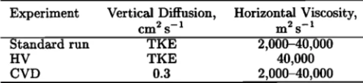
364 AUMONT ET AL.: NUTRIENT TRAPPING: A DYNAMIC SOLUTION
Table 1. Summary of the Dynamic Experiments.
Experiment Vertical Diffusion, Horizontal Viscosity,
cm 2 s- 1 m 2 s- 1
Standard run TKE 2,000-40,000
HV TKE 40,000
CVD 0.3 2,000-40,000
TKE denotes the pronostic model of vertical tubulence pro-
posed by Gaspar et al. [1990] and by Blanke and Delecluse
[1993].
First and second
values
for horizontal
viscosity
coeffi-
cients are their values at the equator and outside the tropical
regions, respectively.
alent to a decrease of the resolution. Much poorer res- olution alters equatorial dynamics simply because the grid size is too large to correctly resolve, meridionally, the fine-scale equatorial currents such as the EUC or the NECC. Thus our case HV infers only some of the
changes due to using a coarser resolution; a full coarse-
resolution model would perform more poorly.
In the second sensitivity test, OPA was run without the prognostic parameterization of vertical turbulence. Instead, one vertical diffusion coefficient is defined a
priori as equal to 0.3 cm
2 s -• everywhere
within the
ocean. We term this as case CVD. Both sensitivity tests were performed with the on-line version of OPA. Resulting monthly averaged dynamic fields were used to drive the off-line version of the model, as in our standard
run.
Figure I includes sections of the zonal velocity field for both sensitivity tests. In case HV, zonal currents, especially the EUC and the NECC, are, on average, slower than in the standard case. Along 150øW, the
maximum speed of the EUC is about 0.85 ms -• in- stead of about I m s-• in the standard case. A decrease in the intensity of the EUC was also found in a simi-
lar experiment by Maes et al. [1997]. Consequently,
the predicted SEC does not present the two distinct
maxima both observed and simulated in the standard
case. Instead, th.e SEC reaches its maximum speed right
at the equator. In case CVD, abandon of the TKE scheme produces a much more intense SEC. Weaker
near-surface vertical mixing decreases the Ekman layer
depth and thus the vertical dissipation. Consequently,
horizontal near-surface velocities are stronger [Blanke and Delecluse, 1993]. On the other hand, vertical mix-
ing below the mixed layer is more intense in case CVD than in the standard case. The core of the EUC is then slower and shallower [Blanke and Delecluse, 1993]. Fur-
thermore, this current extends about 50 m deeper than in the standard case. At the surface, both sensitivity tests predict a zonal velocity field that does not com- pare as well with the drifter-derived climatology from
Reverdin et al. [1994] as does the field simulated in the standard case (Figure 2). In particular, the SEC pre-
dicted in case HV does not exhibit a minimum along the equateur, which results from an EUC that is too slow. In case CVD, zonal speeds of the SEC are too high.
They can exceed 0.8 m s -• , whereas in the climatology, maximum speeds are about 0.4 m s -•.
Figure 4 includes the water mass budgets for both sensitivity tests. In case HV, water fluxes exhibit two major differences relative to those from the standard case. First, the EUC is weaker, bringing in 29.5 Sv instead of 33.3 Sv for the standard case. This decrease is not apparent in the total mass transport between 50 and
430 m because the deepest part of the westward flowing
$EC is also slower in case HV (Figure 1). Secondly, in case HV, upwelling from the deep ocean (i.e., at the
base of deep box) increases ninefold, to 1.8 Sv. In case
(•VD, the most
noticeable
difference
is the 36% increase
in upwelling at 50 m. Such a result might be expected,
given the study by Blanke and Delecluse [1993] who
show a 66% increase of the near-surface upwelling at
the equator in a tropical Atlantic version of OPA, when
a more classical Richardson number based sch'•me is
used instead of TKE to describe vertical turbulence. The slower horizontal near-surface velocities with the TKE scheme leads to a weaker near-surface upwelling. In the surface box, the zonal mass transport at 130øW is not substantially different from that of the standard case, despite a much faster SEC. In fact, the shallower
EUC compensates this increased eastward transport. In
the intermediate box, the larger vertical extent of the
EUC explains the slightly increased eastward transport
relative to the standard case, despite slower maximum zonal velocities.
Figure 6 includes an equatorial section of total phos- phorus for each of the two sensitivity runs. Case HV exhibits a substantial increase in nutrient trapping. For example, total phosphorus concentrations exceed 4.4
•molL -• at 400 m along the American coast; in the
standard run, total P concentrations reach, at most,
3.7 •molL -• . Since the EUC is weaker, upwelled
waters are more efficiently enriched in nutrients from remineralization of sinking particles. As a consequence, mean phosphorus concentration in the intermediate box
is 0.34 •mol L -• higher
than in the standard
case
(Fig-
ure 7b). Case HV's P-enriched EUC causes P transport
by that current to be 19% higher, despite the lower EUC
intensity. Thus waters upwelled to the surface in case HV have a much higher nutrient content. Resulting
higher export production (+ 11%) and the larger inflow
of nutrient-rich waters from the deep ocean explain in- creased nutrient trapping.
For case CVD, there is no increase in nutrient trap- ping. Surprisingly, maximum phosphorus concentra-
tions (3.4 •umol
L -1 ) are even lower than in the stan-
dard case (3.7 •molL -• ). Such a result is difficult
to explain using the Najjar et al. [1992] analysis (Fig- ure 8), which suggests that a more intense near-surface
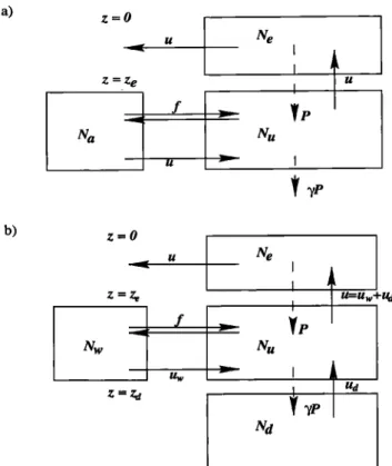
AUMONT ET AL.: NUTRIENT TRAPPING: A DYNAMIC SOLUTION 365 a) z=O Z -'Z e b) z=O
z=z•
•yp
I U=Uw+U
d
Figure 8. (a) Box model redrawn from Najjar et al. [1992] to determine processes involved in nutrient trap-
ping. N•, Ne, and Na represent the nutrient concentra-
tions (t•molm
-a) of the upwelled
waters,
the euphotic
zone, and the region from which the upwelled waters
originate (ambient waters), respectively. P is the pro-
duction
exported
below the euphotic
zone (mols
-•); 7
is the fraction of P that is not remineralized within the divergence zone; u is the intensity of the divergence
(m a s -•); and f is the mixing intensity
between
the up-
welled
waters
and the ambient
waters
(m a s -•). (b) Our
revised version of the box model. The reservoir corre- sponding to the ambient waters (formerly with nutri-
ent concentration Na) has been split into two separate
reservoirs that act in an opposing manner upon nutri- ent trapping. These are the western Pacific and the deep ocean, whose nutrient concentrations are denoted as N•o and Nd, respectively. New advective terms de- scribe transport by the EUC u•o, upwelling of abyssal
waters ud, and near-surface upwelling us, all in units of
m a s -•. Other processes and symbols included in our
revised model are identical to those in Figure 8a.
upwelli. ng, such as found in this case, should increase
nutrient trapping. The nutrient budget (Figure 7c) al-
lows a better understanding. Although near-surface up-
welling is greater, so is the intensity of the EUC because of its larger vertical extent. The EUC's increase in flow
is modest at 130øW (about 5%) but at 150øW, closer to
the source, the EUC is 12% stronger than in the stan-
dard case. As a consequence, the dilution induced by
the EUC is stronger, so that nutrient concentrations of
the upwelled waters are about 0.2/•mol L -1 lower than
in the standard case. Thus, despite greater upwelling,
export production remains almost unchanged (less than
a 2% increase). In the deepest box, the downwelling
(0.5 Sv) of less nutrient rich water than in the stan-
dard case compensates the more than doubled inflow from the deep ocean. Such result shows that different circulations can result in a significant decrease in nu- trient trapping. However the circulation predicted in case CVD is less realistic than in the standard case. Thus a more realistic circulation is a sufiq•ient but not a necessary condition to reduce nutrient trapping.
4. Discussion
4.1. Nutrient Trapping: The Dynamic Solution
Nutrient trapping is highly sensitive to the excess up- welling of abyssal water into the upper equatorial Pa- cific. Our case HV shows that the rate of a model's
abyssal upwelling is linked to its viscosity coefficients,
which are tied to the model's chosen horizontal reso- lution. Coarse-resolution models that simulate nutri-
ent trapping produce excess upwelling of abyssal wa-
ter to the surface tropical Pacific, roughly 4 Sv in the GFDL model [Toggweiler et al., 1991; Toggweiler and
Samuels,
1993] and 10 Sv in the LSG model [Maier-
Reimer et al., 1993]. Coral records
of •4C show that
such upwelling
is unrealistic
[Toggweiler
et al., 1991].
Excess upwelling of abyssal water directly influences nutrient trapping. By bringing up large amounts of
phosphate-rich deep water to the surface equatorial Pa-
cific ocean, deep upwelling of abyssal waters enhances
export production,
which enhances
middepth
PO4
a-
concentrations
and thus the supply
of PO4
•- to the
equatorial divergence. Fewer nutrients are able to es- cape the system.
Nutrient trapping is also related to the intensity of
EUC. Yet the EUC acts indirectly because it lies above
regions where nutrient trapping occurs. By advecting waters originating from the western part of the equa- torial Pacific Ocean, the EUC dilutes the nutrient-rich waters that are upwelled to the surface. In that man- ner, EUC limits the intensity of export production and
thus the amount of nutrient released during remineral-
ization in subsurface waters. Despite stronger near sur-
face upwelling in case CVD, a corresponding increase
of the intensity of the EUC maintained export produc- tion at a level similar to that found in the standard case. Conversely, decreased EUC flow in case HV re-
sults in a substantial increase of phosphorus below the
divergence and, consequently, in a significant increase
(+16%) of export production relative to the standard
case. Coarse-resolution models are capable of produc-
ing only a weak EUC: a maximum speed of less than