Dynamic rate-control and scheduling algorithms for quality-of-service in wireless networks

Dynamic Rate-Control and Scheduling Algorithms for

Quality-of-Service in Wireless Networks

by

Murtaza Abbasali Zafer

B.Tech., Electrical Engineering, Indian Institute of Technology, Madras

S.M., Electrical Engineering and Computer Science, MIT

Submitted to the Department of Electrical Engineering and Computer Science

in partial fulfillment of the requirements for the degree of

Doctor of Philosophy in Electrical Engineering and Computer Science

at the

MASSACHUSETTS INSTITUTE OF TECHNOLOGY

September 2007

@

Massachusetts Institute of Technology 2007. All rights reserved.

Author ...

....

...

Department of Electrical Engineering and Computer Science

June 21, 2007

-- I

I

Certified by...

...

.d...

Eytan Modiano

Associate Professor

Thesis Supervisor

Accepted by..

MASSACHUSETTS INST OF TEOHNOLOGY

CT

I

UIBR ARIES

... ... ... ...

. ....

.. .. ..:

...

...

Arthur C. Smith

Chairman, Department Committee on Graduate Students

Dynamic Rate-Control and Scheduling Algorithms for Quality-of-Service

in Wireless Networks

by

Murtaza Abbasali Zafer

Submitted to the Department of Electrical Engineering and Computer Science

on June 21, 2007, in partial fulfillment of the

requirements for the degree of

Doctor of Philosophy in Electrical Engineering and Computer Science

Abstract

Rapid growth of the Internet and multimedia applications, combined with an increasingly

ubiquitous deployment of wireless systems, has created a huge demand for providing

en-hanced data services over wireless networks. Invariably, meeting the quality-of-service

re-quirements for such services translates into stricter packet-delay and throughput constraints

on communication. In addition, wireless systems have stringent limitations on resources

which necessitates that these must be utilized in the most efficient manner. In this

the-sis, we develop dynamic rate-control and scheduling algorithms to meet quality-of-service

requirements on data while making efficient utilization of resources. Ideas from Network

Calculus theory, Continuous-time Stochastic Optimal Control and Convex Optimization are

utilized to obtain a theoretical understanding of the problems considered, and to develop

various insights from the analysis.

We, first, address energy-efficient transmission of deadline-constrained data over

wire-less fading channels. In this setup, a transmitter with controllable transmission rate is

considered, and the objective is to obtain a rate-control policy for transmitting

deadline-constrained data with minimum total energy expenditure. Towards this end, a deterministic

model is first considered and the optimal policy is obtained graphically using a novel

cu-mulative curves methodology. We, then, consider stochastic channel fading and introduce

the canonical problem of transmitting B units of data by deadline T over a Markov fading

channel. This problem is referred to as the "BT-problem" and its optimal solution is

ob-tained using techniques from stochastic control theory. Among various extensions, specific

setups involving variable deadlines on the data packets, known arrivals and a Poisson arrival

process are considered. Using a graphical approach, transmission policies for these cases

are obtained through a natural extension of the results obtained earlier.

In the latter part of the thesis, a multi-user downlink model is considered which consists

of a single transmitter serving multiple mobile users. Here, the quality-of-service

require-ment is to provide guaranteed average throughput to a certain class of users, and the

objective is to obtain a multi-user scheduling policy that achieves this using the minimum

number of time-slots. Based on a geometric approach we obtain the optimal policy for a

general fading scenario, and, further specialize it to the case of symmetric Rayleigh fading

to obtain closed-form relationships among the various performance metrics.

Thesis Supervisor: Eytan Modiano

Title: Associate Professor

Acknowledgments

As I look back on the years spent at MIT, I recall the moments of fun, play and learning,

that have all together made this an immensely memorable endeavor. I realize the value of

this opportunity and the change it has brought in my life, both in terms of professional

and intellectual development. It is an honor and pleasure to have participated in this

process, and I would like to express gratitude towards everyone and everything that made

this happen.

First and foremost, I would like to profoundly thank my advisor, Prof. Eytan Modiano,

for his invaluable guidance in research and career, and the fun we had as a research group. I

relish the relationship that we have developed over these years and look forward to continue

to seek his advice in the future; I thank him in advance for it. I would also like to express

gratitude to my thesis committee members, Prof. Sanjoy Mitter, Prof. Asuman Ozdaglar

and Prof. Devavrat Shah, for valuable comments and suggestions on the research work. In

the Spring of 2006, it was a pleasure to work with Prof. John Wyatt as a teaching assistant

and I would like to thank him for giving me this opportunity. I really appreciate his belief

in intuition and the wonders it can bring in understanding and solving problems.

The other important part of my experience at MIT was the diverse set of people that I

met and the friendships that I made over these years. I would like to thank all my friends

and colleagues for their support and encouragement. Thanks to Anand Srinivas for adding

'unlimited' humour at and outside of work; I would always cherish his friendship and the

times we spent together. Thanks to my other wonderful office mates, Andrew Brzezinski

and Jun Sun, who were equal partners in the 'crimes' (read 'fun'), that included tennis,

T.T. sessions, lunches, tea/coffee breaks and long 'enlightening' discussions. Thanks to

Zeeshan Syed, Ebad Ahmed, Shashibhushan Borade and Siddhartha Jain for making S&P

inhabitable and a fun place to live in. Thanks also to Sonia Jain, Masha Ishutkina, Dr.

Gil Zussman, Prakash Pottukuchi, S. Krishnakumar, Krishna Jagannathan, Guner Celik,

Ajay Deshpande, Saif Khan, Raj Rao, Siddharth Ray, Jay-kumar Sundararajan, Amit

Deshpande, Rehan Tahir, Saad Zaheer, Danish Maqbool and others, for the enjoyable and

memorable times spent together.

My deepest gratitude is for my parents, Abbas and Mehjabeen Zafer, for their

unwa-vering support, love and encouragement, and above all, the sacrifices they have made for

me; words will never be able to describe my appreciation for them. I would also like to extend my deepest thanks to my brother, Ali Zafer, for all his advices that have and will continue to shape my life. Thanks to my sister, Zainab, for her love and support, and my sister-in-law, Sadaf. My gratitude for my grand-parents and others in the family (especially my aunt Khudammi) who have been an integral part of the support and encouragement that I have received. My deepest thanks to my loving fiancee, Samreen, for her love and support during the latter years at MIT, as I look forward to spending my life with her.

I am grateful to the various funding agencies for their financial support for this re-search work. In particular, this work was supported by NSF ITR grant CCR-0325401,

by DARPA/AFOSR through the University of Illinois grant no. F49620-02-1-0325, by NASA Space Communication Project grant number NAG3-2835, by ONR grant number

Contents

1 Introduction

1.1 Deadline-Constrained Energy-Efficient Rate Control

1.1.1

Problem Overview

1.1.2 Related Work ...

1.1.3

Contributions . . .

1.2 Multi-user Scheduling with

1.2.1

Problem Overview

1.2.2 Related Work . . .

1.2.3

Contributions . . .

1.3 Thesis Organization . . .

. . . .

. . . .

. . . .

Throughput-rate Guarantees .

. . . .

. . . .

. . . .

. . . .

2 Deadline-Constrained Data Transmission

-

Deterministic

2.1 Introduction . . . .

2.2 System Model . . . .

2.2.1

Data Flow Model . . . .

2.2.2 Transmission Model . . . .

2.3 Time-Invariant Power-Rate Function . . . .

2.3.1

Problem Formulation . . . .

2.3.2

Optimality Properties . . . .

2.3.3

Optimal Policy . . . .

2.4 Time-varying Power-Rate Function . . . .

2.4.1

Problem Formulation . . . .

2.4.2 Optimality Properties . . . .

2.5 Chapter Summary . . . .

Setup

27

27

28

28

31

31

32

32

37

44

45

45

3 Stochastic Setup - "BT-problem" 53 3.1 Introduction . . . . 53 3.2 System Model . . . . 54 3.2.1 Transmission Model . . . . 55 3.2.2 Channel Model . . . . 56 3.3 BT-problem . . . . 58

3.3.1 Optimal Control Formulation . . . . 58

3.3.2 Optimality Conditions . . . . 60

3.3.3 Optimal Transmission Policy . . . . 62

3.4 BT-problem with Short-term Power Limits . . . . 68

3.4.1 Problem Formulation . . . . 68

3.4.2 Optimal Policy . . . . 70

3.4.3 Simulation Results . . . . 79

3.5 Chapter Summary . . . . 81

4 Stochastic Setup - Variable Deadlines and Arrivals 83

4.1 Introduction . . . .

83

4.2 Cumulative Curves Generalization . . . .

84

4.2.1 System Model . . . . 84

4.2.2 Problem Formulation . . . . 85

4.2.3 Variable Deadlines Setup . . . . 87

4.2.4 Arrivals with a Single-Deadline Setup . . . . 90

4.2.5 Arbitrary Packet Arrivals - BT-Adaptive Policy . . . . 93

4.3 Stochastic Arrivals . . . . 96

4.3.1 Optimal Control Formulation . . . . 97

4.3.2 Constraint Relaxation . . . . 99

4.3.3 Simulation Results . . . . 103

4.4 Chapter Summary . . . . 106

5 Multi-user Scheduling with Throughput-rate Guarantees 109 5.1 Introduction . . . . 109

5.2 System and Problem Description . . . . 110

5.2.2

Problem Description . . . .

111

5.3 Optim al Policy . . . 113

5.4 Dimensioning . . . 118

5.4.1

Throughput Characterization . . . .

118

5.4.2

Comparison with Random-scheduling Policy . . . .

122

5.5 Simulation Results . . . .

123

5.6 Chapter Summary . . . .

128

6 Conclusion

129

A Proofs for Chapter 2

131

A.1 Proof of Theorem II - Uniqueness . . . . 131

A.2 Proof of Theorem III - Minimal Maximum Power . . . . 132

A.3 Proof of Lemma 5 . . . 133

A.4 Proof of Lemma 7 . . . . 133

A.5 Proof of optimality of the algorithm . . . .

134

A.6 Algorithm for constructing DOP'(t) when A(t) and Dmin(t) are piecewise

con-stant functions . . . .

135

A.7 Proof of Lemma 8 . . . .

137

B Proofs for Chapter 3

139

B.1 Verification Theorem for the BT-problem in Section 3.3 . . . 139

B.2 Proof of Theorem VI - BT-problem . . . . 143

B.3 Proof of Lemma 18 - Existence and Uniqueness of the solution to the ODE in (B.17) ... .. ... 147

B.4

Proof of Lemma 19 - Functions {f2(s)} are the unique solution of the ODE system in (B.21) . . . . 149

B.5

Proof of Lemma 21 - Uniform convergence of (ff)'(s) . . . . 150

B.6 Proof of Theorem VII - Constant Drift Channel, Monomial Case . . . . 154

B.7 Proof of Theorem VIII - Constant Drift Channel, Exponential Case . . . . 154

B.8 Proof of Lemma 10 - Weak Duality . . . . 158

B.10 Proof of Theorem X - BT-problem with Power Constraints and Constant D rift Channel . . . .

B.11 Proof of Theorem XI - Strong Duality . . . .

B.12 Computation of ArJ(x, c, t) given in (3.12) . . . . C Proofs for Chapter 4

C.1 Proof of Theorem XII - Variable Deadlines Case . . . . .

C.2 Proof of Theorem XIII - Arrivals with Single-Deadline

C.3 Boundary Condition for the Poisson Arrivals Problem

C.4 Proof of Lemma 11 . . . .

D Proofs for Chapter 5

D.1 Proof of Lemma 12 . . . . D.2 Proof of Lemma 13 . . . . D.3 Proof of Theorem XV . . . .

D.4 Proof of Lemma 16 . . . .

D.5 Proof of Theorem XVII . . . .

167 .167 . . . . 176 . . . . 184 . . . . 185 187 . . . . 187 . . . . 188 . . . . 190 . . . . 192 . . . . 192 161 162 165

List of Figures

1-1 A schematic diagram of the system model for the deadline-constrained,

energy-efficient, data transmission problem . . . .

19

1-2 Transmission power as a function of the rate and the channel state; (a) fixed

channel state, (b) variable channel state. . . . .

20

1-3 A schematic diagram of the system model for the multi-user scheduling problem. 23

2-1 Data flow model: (a) Fluid arrival model, (b) Packetized arrival model

.

.

29

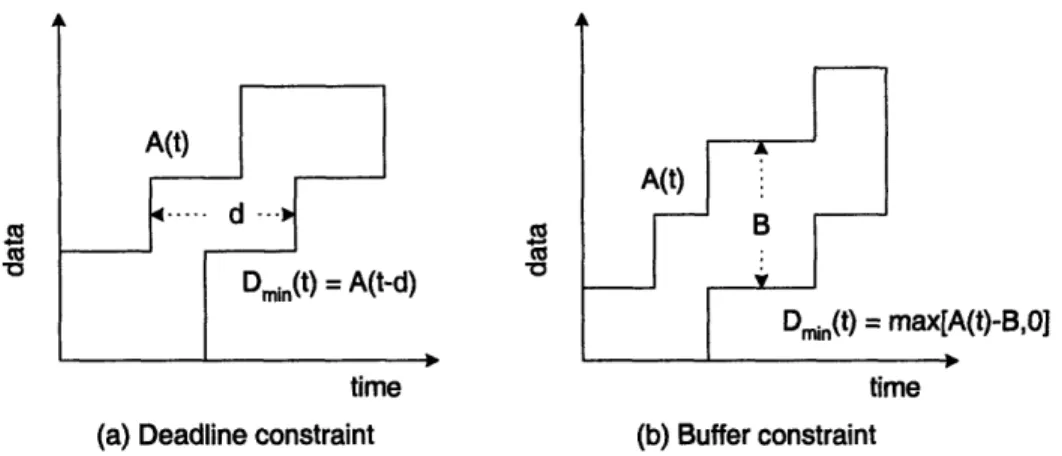
2-2 QoS Examples: (a) Packet deadline constraint of d, (b) Buffer constraint of B. 30

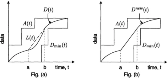
2-3 Figure for Theorem I: (a) an admissible departure curve D(t) and (b) the

new curve D"ew(t). . . . . 35

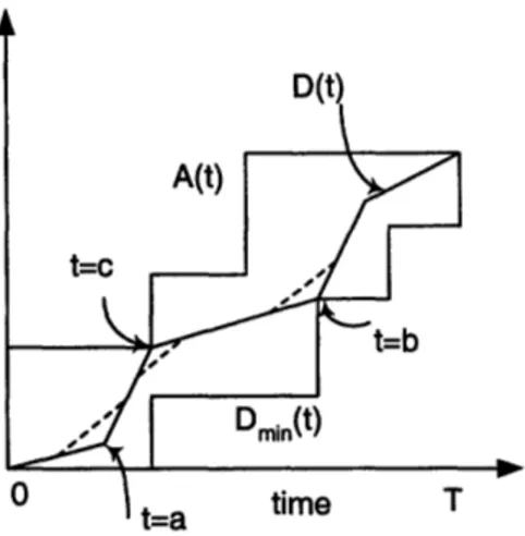
2-4 Example showing violation of Lemmas 2-4. The dotted line shows that D(t)

does not meet the optimality criterion. . . . .

36

2-5 String visualization for the optimal curve, (a) string lying between A(t) and

Dmin(t); (b) D Pt(t) as taut string. . . . . 38

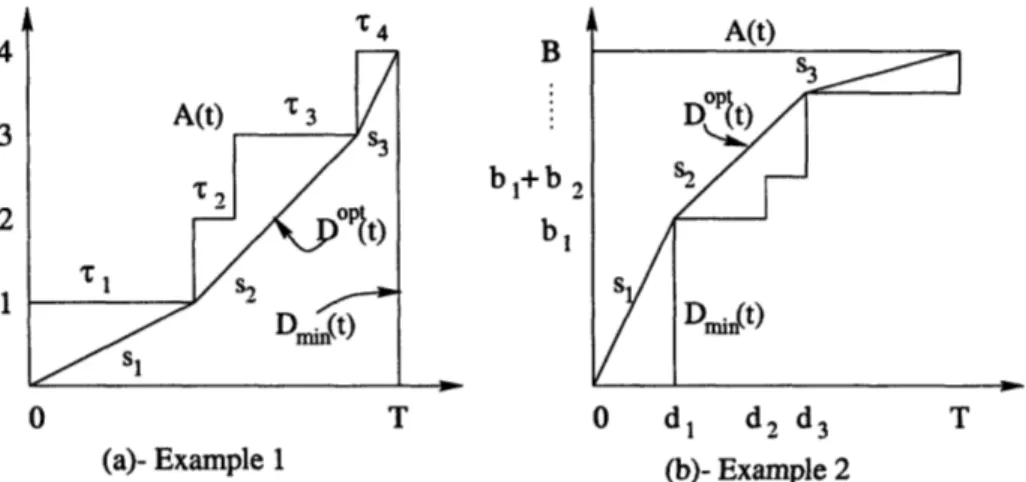
2-6 Curves A(t), Dmin(t) and DOPt (t)

for Examples 1 and 2. . . . .

40

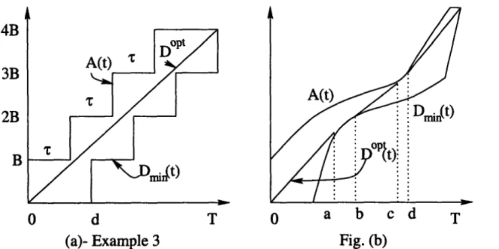
2-7 Curves A(t), Dmin(t) and D ~t(t) for (a) Example 3 and (b) Continuous data

flow. ...

...

41

2-8 Example depicting A(t), Dmin(t) and the constructed D(t). . . . . 43

3-1 Modulation scheme considered in

[40]

as given in the table. The

correspond-ing plot shows the least squares monomial fit, 0.043r2.

67

_{, to the scaled}

piece-wise linear power-rate curve. . . . .

55

3-2 Schematic description of the system for the BT-problem. . . . .

58

3-3 System evolution over time for the BT-problem. . . . .

59

3-4

fb(T

-

t) and fq(T

-

t) plot for the bad and the good channel respectively.

Other parameters include, g(r) = r2_{, T = 10, A = 5, -y = 0.3. . . . . 65}

3-5 Expected energy cost for the optimal and the direct drain (DD) policy. . .

.

65

3-6 Total cost comparison of the optimal and the full power policy. . . . .

79

4-1 Cumulative curves for (a) BT-problem, (b) Variable deadlines case . . . . .

88

4-2 Cumulative curves for the arrivals with a single deadline case. . . . .

91

4-3 Energy cost comparison for Poisson arrival process for (a) different arrival

rate, (b) different sample paths. . . . .

95

4-4 Energy cost versus packet deadline for Poisson arrival process . . . .

95

4-5 Energy cost versus packet size for Uniform arrival process. . . . .

96

4-6 Plot of f(t) forT=10, ro= 1, (= 1, B=1 andg(r)=er -1. . . . . 100

4-7 (a) Comparison of expected energy cost for RP and Optimal policy. (b)

Comparison of rate at t

=

0 as a function of the buffer size x.

. . . .

102

4-8 Plot comparing the expected energy expenditure of RP and DD policies and

the percentage gain ((DDcost-RPcost)*100/DDcost).

. . . .

104

4-9 (a) Comparison of energy expenditure for 100 sample paths at (

=

1. (b)

Comparison of average buffer size over time for

= . . . .

104

5-1 The Z1 region for N = 3, threshold vector i = (al, a2, a3) and Q = R+N

Note that Zf = {F: 0 < ri

aj, Vi = 1, ... , N}.

. . . .

114

5-2 Optimal policy structure for

N = 3, threshold vector

5

= (al, a2, a3) and

Q = R+N. The Zi regions are top truncated pyramids. . . . .

116

5-3 Plot of R/p versus N for the optimal policy for various -y values. . . . .

121

5-4 Plot of R/I versus -y for values of N = 1,2,4,8,14. . . . . 121

5-5 Running time-average of throughput rate for Rayleigh fading with 3 QoS users, R = 200 Kbits/sec. . . . . 124

5-6 Throughput gain, RPt/Rr, for Rayleigh fading with y = 0.3. . . . . 125

5-7 Running time-average of throughput rate for Nakagami fading with fade

pa-rameter m = 0.6, -y = 0.3 and 3

QoS

users . . . . 125

5-8 Throughput gain, RPt

/Rr,

for Nakagami fading with fade parameter m = 0.6 and -y = 0.3. . . . 125

5-9 Comparison of the fraction of slots utilized by the random, OPF, TDMA and

optim al policies. . . . 126

C-1 Proof of Theorem XII for the two packet case, (a) case

B

and

(b) case

_{A20-f(Tl-t)...6}1

. .

168

C-2 Proof of Theorem XIII for the two packet case, (a) case

A2 > A

and (b) case

1

.

.i . . . 177

D Fw t m ff(Ti-t) he.proof.of.Lemma.13 .... . ... 189

Chapter 1

Introduction

Communication technology has advanced rapidly over the last few decades, from

point-to-point telegraphic services to modern wired-telephone and computer networks, and now

expanding to wireless systems. While the earlier telephone systems were designed primarily

for voice communication, present day communication networks handle a large volume of data

traffic which is expected to further grow exponentially, fuelled by the rapid growth of the

Internet and multimedia applications. Data services are expected to expand beyond email

and web-data transfers to more enhanced services such as video and real-time multimedia

streaming, delay-constrained file transfers and Voice-over-IP (VoIP) [1]. To deliver these

services there are various wireless data systems under development that include, for example,

1xEV-DO/HDR [3], 3G/4G and WiMAX systems. Applications involving delay constraints

also arise in other communication systems such as sensor and mobile ad-hoc networks. For

example, in real-time monitoring scenarios using sensor networks, the data collected by

the sensor devices must be transmitted back to a central processing node within a certain

fixed time-interval. Invariably, providing such enhanced Quality-of-Service (QoS) translates

into stricter delay and throughput requirements on communication, thus, introducing new

problems and challenges in addressing these concerns.

As compared to the wire-line networks, communication over wireless channels

inher-ently involves dealing with time-varying and stochastic channel conditions and scarcity of

resources. Time-varying channel conditions arise due to a variety of reasons, most common

being multi-path fading, shadowing and weather conditions in case of satellite

communica-tion [4,5]. Due to the time-varying nature of the channel gain and interference from other

sources, the signal-to-noise power at the receiver fluctuates over time which translates into a time-varying rate at which data can be reliably received for a certain bit-error probability. In addition to the channel variability, wireless systems also have more stringent limitations on resources such as battery energy, bandwidth etc., and therefore it necessitates that these must be utilized in the most efficient manner.

In this thesis, we develop dynamic rate-control and scheduling algorithms to meet quality-of-service requirements on data while making efficient utilization of resources. We adopt a theoretical viewpoint and obtain optimal solutions under various setups, utiliz-ing techniques from Network Calculus [50-53], Continuous-time Stochastic Control the-ory [63-65] and Convex Optimization [66}. In Chapters 2, 3 and 4, we consider a point-to-point wireless link model and treat various formulations in which the objective is to minimize the total transmission energy expenditure when packets have strict deadline constraints. In Chapter 5, we consider a wireless down-link model where there is a single transmitter serv-ing multiple mobile users and the objective is to obtain a multi-user schedulserv-ing policy that minimizes the total time-slot utilization while providing throughput-rate guarantees.

For the remainder of this chapter, we delve into a more detailed overview of the prob-lems addressed in the thesis, outline the related work in the literature and describe our contributions. Finally, we conclude the chapter with an outline of the thesis.

1.1

Deadline-Constrained Energy-Efficient Rate Control

1.1.1 Problem Overview

Energy consumption is an important concern in wireless system design

[2,8-13,21,22,26-28,41, 48] and minimizing the total energy expenditure has numerous advantages in terms

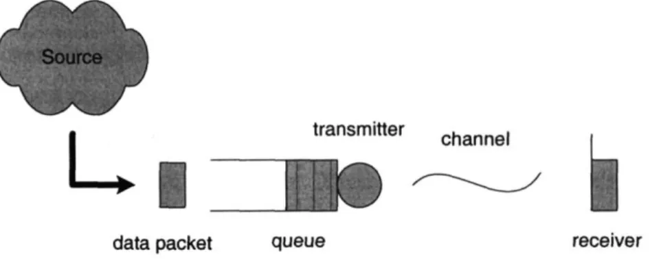
of efficient battery utilization for mobile devices, increased lifetime of sensor devices and mobile ad-hoc networks, and better utilization of limited energy sources in satellites. Since in most scenarios the energy spent for transmission constitutes the bulk of the total energy expenditure, it is imperative to minimize this cost to achieve significant energy savings. The work presented in Chapters 2, 3 and 4, addresses energy-efficient transmission of data over a wireless channel with deadline constraints. Broadly speaking, we consider a point-to-point wireless link model with strict deadline constraints on data transmission and utilize dynamic rate-control to minimize the total transmission energy cost. A schematic diagram

transmitter _channel

data packet queue receiver

Figure 1-1: A schematic diagram of the system model for the deadline-constrained, energy-efficient, data transmission problem

of the setup is shown in Figure 1-1.

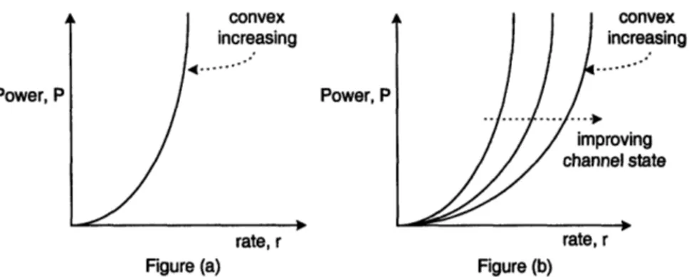
To understand how transmission energy expenditure can be minimized using rate con-trol, we need to look at the power-rate function. The power-rate function defines the relationship that specifies the amount of transmission power required to reliably transmit at a certain rate. Two fundamental aspects of this function, which are exhibited by most encoding/communication schemes and hence are common assumptions in the literature are as follows [4,8-13,21,22,27,29,32,39,401. First, for a fixed bit-error probability and channel state, the required transmission power is a convex function of the data rate, as shown in Figure 1-2(a). This implies, from Jensen's inequality, that transmitting data at low rates, over a longer duration, is more energy efficient as compared to high rate transmission. Second, the wireless channel is time-varying which shifts the convex power-rate curve as a function of the channel state as shown in Figure 1-2(b). As good channel conditions require less transmission power, one can exploit this variability over time by adapting the rate in response to the channel conditions. Thus, we see that by adapting the transmission rate intelligently over time, energy cost can be reduced.

Modern wireless devices are equipped with channel measurement and rate adaptation capabilities [3,4,6,7]. Channel measurement allows the transmitter-receiver pair to mea-sure the fade state using a pre-determined pilot signal while rate control capability allows the transmitter to adjust the transmission rate over time. Such a control can be achieved in various ways that include adjusting the power level, symbol rate, coding scheme, con-stellation size and any combination of these approaches; furthermore, in some technologies the receiver can detect these changes directly from the received data without the need for an explicit rate change control information [7]. In present systems, the transmission rate

Power, P

rate, r

Figure (a) Figure (b)

rate, r

Figure 1-2: Transmission power as a function of the rate and the channel state; (a) fixed

channel state, (b) variable channel state.

can be adapted very rapidly over millisecond duration time-slots [3,4,6], thereby, providing

ample opportunity to utilize rate adaptation to optimize system performance.

Summarizing, for a given transmitter-receiver pair with rate-adaptation capabilities and

the above mentioned power-rate function characteristics, the goal of this research work is

to seek the transmission policy that minimizes the energy expenditure while ensuring that

the strict QoS constraints are met. Throughout the thesis, the terms transmission policy

and rate-control policy will be used interchangeably and they refer to the transmission rate

to be selected for data transmission at a certain time.

1.1.2 Related Work

Transmission power and rate control are an active area of research in communication net-works in various contexts. Power control in cellular CDMA netnet-works has been studied

extensively, but with the primary motivation of mitigating interference and addressing the

"near-far" problem [4,33-35]. Adaptive algorithms for network control have been studied

in the context of network stability [36-40,42-45], wherein, various notions of stability are

addressed, but the primary goal is to ensure that the queue sizes do not grow to infinity.

Scheduling and power control have also been considered in the context of average through-put [46,49,75-77], average delay [8,9,27-29] and packet/call drop probability [30-32]. How-ever, this body of literature considers "average metrics" that are measured over an infinite time horizon and hence do not directly apply for delay constrained/real-time data. Fur-thermore, with strict deadline constraints, adapting the transmission rate simply based on steady state distributions does not suffice and one needs to take into account the system

dynamics over time, thereby, introducing new challenges and complexity into the problem.

Recent work in this direction includes [10-13,20-22,26. The works in [10-12,26] studied

various offline formulations for energy-efficient data transmission by assuming complete

knowledge of the future arrivals and the channel states, and then devised heuristic online

policies using the offline optimal solution. Thus, in this body of work, the sample path was

assumed known for the optimization problem therein. The authors in [13] studied several

data transmission problems using discrete-time Dynamic Programming (DP) [61], however,

the problems that we consider in this work become intractable using this methodology due

to the large state space in the DP-formulation or the well-known "curse of dimensionality".

In [21], the authors considered packet deadlines and transmission over a time-invariant

(non-fading) channel and used filtering techniques to obtain the energy efficient policy, while, the

formulation in [22] allowed energy recovery when the transmitter is in the idle state. As

we see later, the generalized formulation that we consider in Chapter 2 recovers back the

results in [10,21] as special cases.

Job scheduling with deadlines has also been considered in the Operations Research

literature. Recent relevant work here includes [23-25] which deal with scheduling of jobs

(or packets) with hard deadlines, where the service rate is fixed and the goal is to maximize

the number of packets that get served. However, the difference in the system model for our

case is that the service rate (transmission rate) is controllable and there is a power cost

associated with using a particular service rate; furthermore, there is no dropping of packets

and the goal is to minimize the total energy cost of transmission.

1.1.3 Contributions

We consider two different setups for the rate control problem - the Deterministic Setup and the Stochastic Setup. In Chapter 2, we consider the deterministic setup in which all time-variability in the system is known in advance and the goal is to seek the optimal off-line solution. Here, we describe the data flows in and out of the transmitter queue using cumulative curves, namely, the Arrival Curve and the Departure Curve; and model the

quality-of-service (QoS) constraints using a new notion of a Minimum Departure Curve.

Using this framework, we obtain the optimal policy for a general formulation that incor-porates a wide set of QoS constraints in the problem, hence, some of the earlier results in the literature can be recovered as special cases from our general formulation. We also

present a graphical visualization of the problem that provides an intuitive and easy way to understand the optimal minimum-energy transmission policy.

In Chapters 3 and 4, we consider the stochastic setup and begin in Chapter 3 with the following canonical problem (which is referred to as the "BT-problem") - the transmitter has B bits of data in the queue which must be transmitted by deadline T over a time-varying and stochastic channel. The channel state is modelled as a Markov process. And, the objective is to obtain the optimal transmission policy that minimizes the expected total energy expenditure. We consider two different formulations here - first in which there is no maximum power limit and the deadline constraint is a hard constraint, and second in which there is an average short-term power limit and the data left in the queue at time T incurs a penalty cost. Using a continuous-time formulation and techniques from Stochastic Optimal

Control [63-65] theory and Lagrangian Duality [66,68], we obtain the optimal transmission

policy for both these setups. From the closed-form structure of the optimal policy, various useful insights into the data transmission problem and results under special scenarios are also obtained. These are further discussed in detail in that chapter.

Finally in Chapter 4, we extend the above results to more generalized scenarios. First, we consider the variable deadlines setup where the packets in the transmitter queue have distinct individual deadlines and the goal is to serve these packets over a stochastic channel with minimum energy. Second, we consider the arrivals with a single deadline case, where there is a stream of known packet arrivals and a single deadline by which all the data must depart. Using the cumulative curves framework as discussed in Chapter 2 and a decomposition approach, we obtain a transmission policy through an intuitive and a natural extension of the previous results. This policy is shown to be optimal under a specific class of channel models. Using the above results, we also obtain an online energy-efficient policy for the case of arbitrary and unknown packet arrivals to the queue with individual packet deadlines. Lastly, we consider a stream of Poisson packet arrivals to the queue and a single deadline by which they must all be transmitted. In this setup, we obtain an energy-efficient transmission policy in closed-form, and also highlight the various insights that can be drawn from it regarding the effect of statistical knowledge of the packet arrivals on energy expenditure.

We have presented part of the results from Chapter 2 in [14,15], from Chapter 3 in [18,19] and from Chapter 4 in [14,16,17].

- -channel mobile user

mobile usurs

base station

-.

base station

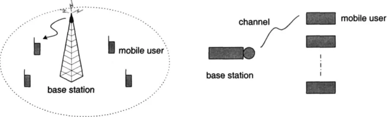
-Figure 1-3: A schematic diagram of the system model for the multi-user scheduling problem.

1.2

Multi-user Scheduling with Throughput-rate Guarantees

1.2.1

Problem Overview

As mentioned earlier, wireless communication inherently involves dealing with time-varying channel conditions. To mitigate the effects of channel fading, much of the early research fo-cus in cellular networks was to use a variety of diversity techniques such as time interleaving of data, frequency hopping and using power-control in CDMA systems [4]. However, with a single base-station serving multiple mobile users one can take advantage of channel fading

by utilizing another form of diversity, which is referred to as Multi-user Diversity [4,80

or Opportunistic Scheduling [75-79]. The main idea behind this technique is that with multiple mobile-users experiencing independent fading, at any given time there will some users with good channel conditions, and the base-station can then select the "best user" for transmission based on achieving certain required objectives.

In this part of the thesis, presented in Chapter 5, we address multi-user scheduling for Quality-of-Service (QoS) traffic that require a certain guaranteed throughput-rate. We consider a single server that represents the base station transmitting to multiple users that represent the mobile handsets. The system operates in a time-slotted manner and in each time-slot the base station can serve only one user. This setup is referred to in the literature as the Wireless Downlink Scenario, where "downlink" refers to the communication link from the base-station to the mobile user. A schematic diagram of the setup is shown in Figure 1-3. We further assume that the set of users are divided into two classes: (i) throughput-rate guaranteed, QoS users and (ii) "best effort" (BE) users. The QoS users in the system represent session applications such as FTP, high data-rate web-browsing,

throughput-constrained data transfers etc., which require the base station to provide a certain long-term data rate on the downlink. In contrast, the BE users represent on-the-fly applications such as email transfers, low priority and latency tolerant data transfers etc., which do not have rate requirements and are short-lived. The goal of this work is to design a scheduling policy that provides the required throughput rates to the QoS users with the least time-slot utilization and maximizes the remaining fraction of time-slots assigned for the BE class.

1.2.2

Related Work

Downlink scheduling is an active area of research in wireless systems and has been studied in different contexts. The work relevant for our study includes [37-39,75-79). In [37-39], the authors studied the problem within the context of queue stability, wherein, the goal was to ensure that the queue sizes do not grow to infinity. The work in [75] studied opportunistic scheduling under a utility maximization framework and presented various formulations with different objective functions. In [76], the authors considered the objective of maximizing the minimum throughput-rate among a set of users and obtained the optimal policy for that setup, while in [77] the framework was extended to include a dynamic user population. In

[78],

the authors assumed multiple simultaneous transmissions employing spread spectrum and considered fairness constraints while in [79] the authors presented algorithms for scheduling users with average delay considerations.

1.2.3

Contributions

As mentioned earlier, we consider a setup where the set of users are divided into two classes

- the QoS users which are guaranteed certain throughput-rates and the BE users which form the low-priority service. The goal is to obtain a multi-user scheduling policy that serves the QoS users with the least time-slot utilization and maximizes the remaining fraction of slots allocated to the BE class. To solve the problem, we adopt a geometric approach and show that the optimal policy satisfies a special structure. The geometric analysis is valid for a general fading model, and hence, is applicable for a wide set of scenarios. Specializing the results to case of Rayleigh fading, we obtain closed-form formulas that relate the achievable throughput-rate guarantee of the QoS users as a function of other system parameters, thus, providing closed-from relationships to understand the various system tradeoffs. Analytical

comparison between the optimal policy and the random-scheduling policy also shows that

gains on the order of ln(N) can be achieved, where N is the number of QoS users. We have

presented part of the results from Chapter 5 in [73,74].

1.3

Thesis Organization

The rest of the thesis is organized as follows. In Chapters 2, 3 and 4, we consider in detail

the various setups for the energy-efficient transmission rate control problem, as described

briefly in Section 1.1. The deterministic case for this problem is treated in Chapter 2 while

the stochastic setup is presented in Chapters 3 and 4. In Chapter 5, we consider in detail

the multi-user scheduling problem with throughput-rate guarantees as discussed briefly in

Section 1.2. Finally in Chapter 6, we conclude the thesis.

Chapter 2

Deadline-Constrained Data

Transmission

-

Deterministic

Setup

2.1

Introduction

Delay constraints and energy-efficiency are important concerns in wireless data transmission, and as discussed in Chapter 1, these concerns arise frequently in real-time data commu-nication. In principle, without energy concerns, strict deadline constraints can always be met by transmitting at high rates, albeit, incurring high transmission energy expenditure. When the transmitter has energy limitations, then as discussed in Chapter 1, one can utilize transmission rate-control to minimize the energy cost. More specifically, since transmission power is a convex function of the rate, data should be transmitted at low rates but ensuring that the deadline constraint is met. And furthermore, as transmission power also depends on the underlying channel state, the rate should be adapted in response to the channel variations.

In this part of the research work, presented in Chapters 2, 3 and 4, we address the question of optimal rate control to serve deadline-constrained data with minimum energy expenditure. We begin in this chapter by considering a deterministic setup, where the time-variability in the system is assumed known in advance. The problem is formulated over a finite-time horizon using a cumulative curves approach and its optimal policy is obtained.

As will be evident later, such an approach provides an appealing graphical visualization

of the problem and the optimal solution. The formulation also generalizes the problems

considered in [10,21] which can be obtained as special cases, as further discussed later.

The rest of the chapter is organized as follows. In the next section, Section 2.2, we

present the data flow and the transmission model. In Section 2.3, we consider the

time-invariant power-rate function while in Section 2.4 the results are generalized to incorporate

the time-varying power-rate function. Finally, in Section 2.5, we conclude the chapter and

summarize the results.

2.2

System Model

We consider a continuous-time setup and assume that the rate can be varied continuously

over time. Clearly, such a model is an approximation of a communication system which

operates in discrete time-slots. However, the assumption is still justified since in practice

the time-slot durations are very short on the order of 1 msec [3], and much smaller than

packet delay requirements which are usually on the order of 100's of msec. An advantage

of such a model is that it makes the problem mathematically tractable and also provides

a simple and intuitive graphical visualization of the optimal solution. In fact, the results

obtained here can be applied to a discrete-time system in a straightforward manner by

simply evaluating the solution at the slot boundaries.

2.2.1 Data Flow Model

To describe the flow of data into the system, we utilize a cumulative curves methodology

[50, 51, 53]. This model applies to a general setting where data could arrive in packets

(packetized model) or in a continuum of bits (fluid model). Let A(t), D(t) and Dmin(t) denote the arrival curve, departure curve and the minimum departure curve respectively. These curves are assumed right-continuous functions and are defined as follows.

Definition

1

(Arrival Curve) An arrival curve A(t), t > 0, t

E

R, is the total number of

bits that have arrived in time interval [0, t].

Definition 2 (Departure Curve) A departure curve D(t), t > 0, t E R, is the total number of bits that have departed (served) in time [0, t].

Fig. (a) time t 0 Fig. (b) time t

Figure 2-1: Data flow model: (a) Fluid arrival model, (b) Packetized arrival model

In case of a fluid arrival model, A(t) is a continuous function, whereas, for a packet

arrival model it is a piecewise-constant function as depicted in Figure 2-1. To ensure that

the transmitter does not transmit more than the data that has arrived to the queue, we

require that D(t)

A(t). We refer to this as the causality constraint. Now, to model the

quality-of-service constraints we introduce a new notion of a "minimum departure curve"

which is defined as follows.

Definition 3 (Minimum Departure Curve) Given an arrival curve A(t), a minimum

departure curve Dmin(t) is a function such that Dmin(t) 5 A(t),Vt > 0, and is defined as the minimum cumulative number of bits that if departed by time t would satisfy the

quality-of-service requirements.

The function Dmin(t) can be viewed as the constraint function, so that in order to

satisfy the QoS requirements the departure curve D(t) must satisfy D(t) Dmin(t). Thus,

in a compact way the QoS and the causality constraints can be expressed as, Dmin(t) <

D(t) 5 A(t), Vt. Note that the definition of Dmin(t) hides the implicitly assumed service

discipline (the order in which data is served), as the above model looks at the data flow

in a cumulative sense. Through a few illustrative examples, we show next that a number

of commonly used QoS constraints with an appropriate service discipline can be modelled

within this framework.

Delay Constraint: Consider an arrival curve A(t) and a constant deadline constraint d on

all the data. It is clear that by setting, Dmin (t) = 0, t E [0, d) and Dmin (t) = A(t - d), t > d,

and following an earliest-deadline-first service discipline, the deadline constraints will be

satisfied. Thus, here, Dmin(t) is simply a time-shifted version of A(t) as shown in Figure

2-(a) Deadline constraint (b) Buffer constraint

Figure 2-2: QoS Examples: (a) Packet deadline constraint of d, (b) Buffer constraint of B.

2(a). Generalizing this, suppose now that the data has variable deadlines and these deadlines are in the increasing order in which the bits arrive. Consider first a packet arrival model and let {t} denote the arrival epochs, {d"} the deadlines and {bf} the sizes of the packets. Then, Dmin(t) is a piecewise constant function with jumps at times

{tf

= t' + dA} and the sizes of the jumps being

{bi'}.

Similarly, for a continuous data arrival model, let d(t) be the general deadline function, where d(t) is the deadline for data arriving at time t. Assuming that h(s) A s

+

d(s) is a monotonically increasing function, the minimum departure curve

is Dmin(t) = 0, t E [0, d(0)) and Dmin(t) = A(h 1l(t)), t > d(0).

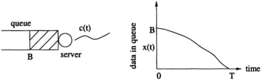
Buffer Constraint: Consider a buffer constraint of B, i.e. the queue size must not exceed

B

Vt > 0. For an arrival curve A(t) and a departure curve D(t) the buffer size at any time t

is given by b(t) = A(t) - D(t). Since b(t) 5 B, we have D(t) max[A(t) - B, 0}. Following

a first-come-first-serve service discipline, it is easy to see that the minimum departure curve must be Dmin(t) = max[A(t) - B, 0] as shown in Figure 2-2(b). It is easy to incorporate a

time varying buffer constraint B(t) as well.

Service- Curve Constraint: The notion of service curves forms an integral part of network

calculus theory [53}. Given a service curve 0(t) and an arrival curve A(t), the minimum departure curve can be obtained as Dmin(t) = A(t) @9 0(t), where ® is convolution in the

min-plus algebra.

Thus, we see that a wide variety of QoS constraints can be abstracted by constructing the appropriate minimum departure curve.

2.2.2

Transmission Model

Let P(t) denote the required transmission power to reliably transmit at rate

r(t)

at time t.

We assume the following power-rate relationship,

P(t) = g(r(t), t) (2.1)

where the function g(r, t) is a convex, increasing function with respect to the first argument

(rate) and g(r, t)

2

0 for r > 0, Vt. The relationship in (2.1) is a general transmission

model for most encoding schemes and has been widely studied in the literature in various

forms [9-13,21,22,27,32]. As a well-known example, the Shannon formula for the power per

bit gives the following relationship, P

=

NoW(2

1

W - 1); in case of other coding schemes

the Shannon formula gives a lower bound on the power per bit.

Given the relationship in (2.1), the transmission energy expenditure of a departure curve

D(t) over time interval [0, T] is given by,

E(D(t)) =

j

g(D'(t), t)dt (2.2)

where D'(t) is the derivative at time t; it gives the transmission rate at that instant' and

the term g(D'(t), t) gives the instantaneous transmission power.

Throughout the paper, our focus will be on the time interval [0, T] for some finite T, and

with finite deadline constraints. Thus, we deal with energy minimization over a finite time

interval rather than considering an infinite time horizon, as done in much of the literature

on power-rate adaptation which studies average performance metrics. Since a departure

curve specifies the transmission rate and vice-versa, we will use the terms departure curve

and transmission policy interchangeably.

2.3

Time-Invariant Power-Rate Function

We first consider the case of a time-invariant power-rate function where P(t) is only a

function of r(t), i.e. P(t)

=

g(r(t)). Such an assumption models a static or a slow fading

wireless channel where over [0, T] the channel gain does not change appreciably over time.

This is a good model for wireless LAN settings and fixed wireless network scenarios.

2.3.1

Problem Formulation

Consider an arrival curve A(t) and assume that this curve is known over the interval [0, T].

Based on the QoS requirements, one can construct the minimum departure curve Dmin(t) as

discussed in Section 2.2. Now given A(t) and Dmin(t) curves, a departure curve D(t) is said

to be admissible if it satisfies both the causality and the QoS constraints; i.e. Dmin (t) <

D(t)

A(t), t E [0, T]. The energy minimization problem is to obtain the admissible

departure curve with the least energy expenditure. Mathematically, this can be stated as

follows,

min E(D (t)) g(D'(t))dt (2.3)

D(t)

_Jo

subject to

Dmin(t) 5 D(t) 5 A(t), t E [0,

T]

D(t) E F

(2.4)

Without loss of generality, we take

Dmin(0) =

0,

Dmin(T) = A(T),

where the last equality

simply states that all the data must depart by T. For admissibility, we also need the

technical requirement that D(t) belongs to the set F, where F consists of all non-decreasing,

continuous functions with bounded right-derivative for all t E

[0, T] and with D(0)

=

0. For

set F, the non-decreasing assumption follows from the cumulative nature of the departure

curves, the continuity assumption is natural as any discontinuity would imply instantaneous

transmission of non-zero amount of data which is practically infeasible and finally, the

bounded right-derivative assumption ensures that the rate and the energy cost in (2.3) are

finite

2

. Furthermore, if one makes the natural assumption that there is no data that arrives

and needs to be transmitted instantaneously, then, admissible departure curves exist.

2.3.2

Optimality Properties

Consider first the following simple example -

the transmitter has B units of data that must

be transmitted by a deadline T. We refer to this as the "BT-problem". This example sheds

important insights into the problem and will also serve as a building block for the general

problem.

2_{Thus, we assume that D'(t) < M,Vt E [0, T], VD(t) E I, where M is chosen large enough such that}

finite-energy practical policies are all included. The curves A(t) and Dmin(t) are also assumed right-continuous with bounded right-derivative for all t E [0, T].

BT-problem: The two curves A(t) and Dmin(t) for this problem are as follows. Since

there are no new arrivals and the queue has B units of data to begin with, the arrival curve

is A(t)

=

B, Vt E [0, T]. Further, there is no minimum data transmission requirement

until the deadline T, at which point all the data must have been sent; hence, we get

Dmin(t) =

0, t E [0, T) and

Dmin(T) =

B. The admissibility criterion specialized to this

case thus becomes 0 < D(t)

<

B and D(T)

=

B. We claim that the optimal policy is

constant rate transmission at rate B/T, i.e. (DQt)'(t) = A and DPt(t) = At, t E

where D (t) denotes the optimal departure curve. To see why this is true consider the

following integral version of Jensen's inequality.

Lemma 1 Let f(t), p(t) be two functions defined for a < t < b such that a < f(t)

0 and

p(t) > 0, with p(t) # 0. Let $(u) be a convex function defined on the interval a < u < /;

then

0 fa

f)p(t)dt

fa $(f)p(t)dt(25

b p(t)dt _{b p(t)dt}

with strict inequality if $() is strictly convex and a

#

b, a

#

/3.

Proof: See [84].

Now, consider an admissible departure curve D(t) and make the following substitution

in the above lemma, p(t)

=

1, $()

= go,

f(

=

D'(), a

=

0 and b

=

T. This gives,

DI

D(t) dt

<

fo

g (D'(t)) dt(26

f

dt

)

f

dt

g (DT

())T

f

g(D'(t))dt

(2.7)

T

0

g(B/T)T < jog(D'(t))dt (2.8)

The left hand side in (2.8) is the total energy cost of the constant rate transmission policy

at rate BIT, while, the right hand side is the total cost of any other admissible departure

curve. The inequality in (2.8) thus proves the optimality claim.

Remark 1 : The result for the BT-problem is fairly intuitive given the convexity property

of the power-rate function. Its practical implication is interesting as it says that for the

time-invariant case there is no gain achieved by a complex variable-rate policy; in fact,

a constant rate policy suffices. Another observation is that when g(-) is strictly convex

the inequality in (2.8) is strict and the constant rate policy is the unique optimal policy. Whereas, for the case of a linear power-rate there is equality in (2.8) and all policies have the same cost.

We now consider the general setup and assume without loss of generality that A(t) > Dmin(t), 0 < t < T. Otherwise, if at some time te there is equality, the problem can be

divided into two sub-problems over time intervals [0, te] and [te, T] and each can be solved independently. The first result, Theorem I, is a generalization of the result for the BT-problem and it gives a criterion for the optimality of a departure curve.

Theorem I (Optimality Criterion) Let D(t) be an admissible departure curve and L(t)

be a straight line segment over [a, b] that joins points D(a) and D(b), 0

<

a < b

<

T. If

L(t) satisfies Dmin(t) L(t) A(t), and, L(t) # D(t), the new departure curve Dnew(t)

constructed as,

Dnew(t)

= D(t), t E [0, a) = L(t), t E [a,b]

=

D(t), t

E

(b, T]

satisfies, E(Dnew(t))

E(D(t)), where the inequality is strict if g(.) is strictly convex.

The above theorem states that if there exists any two points on the curve D(t) that can be joined by a straight line without violating the admissibility constraints, replacing that part of D(t) with the straight line can only lower the energy cost. The implication of this is that whenever admissible, it is optimal to transmit at a constant rate. A schematic diagram depicting this is given in Figure 2-3. Henceforth, the criterion that along a departure curve there does not exist any two points that can be joined by a distinct admissible straight line will be referred to as the "Optimality Criterion".

Proof: First note that since L(t) is admissible, the new curve Dnw(t) is also admissible.

Consider,

E(Dnew(t)) - E(D(t)) = E(L(t)) -

j

g(D'(t),

t)dt (2.9)

Over the interval [a, b], we know from the result for the BT-problem that L(t) has the least energy cost among all departure curves that would transmit (D(b) - D(a)) amount of data

L Dmin(t) _Dmin(t)

a

b time, t

a

b time,

t

Fig. (a)

Fig. (b)

Figure 2-3: Figure for Theorem I: (a) an admissible departure curve D(t) and (b) the new curve Dn'"(t).

result follows.

Remark 2 :(Linear power-rate

function)

An interesting special case arises when the power-rate relationship is linear, i.e. P = nr where n > 0 is a constant. In this case, the inequality in Lemma 1 becomes an equality from which it follows that all departure curves have the same energy cost. Thus, with a linear power-rate curve it does not matter, in terms of energy cost, how the data is transmitted as long as the QoS constraints are met. However, even in the special case of linear power-rate function, we will see next that the departure curve that satisfies the optimality criterion has appealing properties that make it a right candidate for the optimal transmission policy.

Henceforth, we consider the more interesting case of strictly convex g(.) function. The next result shows that the optimal departure satisfying the optimality criterion is unique.

Theorem

II

(Uniqueness) Consider the optimization problem in (2.3) with g(-) being strictly convex. Let D(t) be an admissible departure curve that satisfies the optimality

criterion, then, D(t) is unique and it minimizes the energy cost in (2.3).

Proof: Appendix A.1. U

Throughout now, we will denote the admissible departure curve satisfying the optimality criterion as DOP(t) and later in Section 2.3.3 give an algorithm for constructing D pt(t). We now present the various properties of DPt(t) and start by characterizing the points in time at which the optimal rate changes, i.e. points at which the slope/right-derivative of

t=a

Figure 2-4: Example showing violation of Lemmas 2-4. The dotted line shows that D(t) does not meet the optimality criterion.

DOtP(t) changes, either continuously or in a discrete step. Denoting any such point as to,

the following results follow3.

Lemma 2 At to, DPt(t) either intersects A(t) or it intersects Dmin(t); i.e. we have DOPt (to) =

A(to) or

DPt (to) =

Dmin(to). Note, if there is a discontinuity in A(t) at to

(jump point for packetized data) then DPt (to) = A(to).

Lemma 3 Suppose that at to we have DYPt(to) = Dmin(to), then, the slope change must be

negative.

Lemma

4

Suppose that at to we have D*Pt(to) = A(to) (or A(to)) then the change in slope

must be positive.

The observations in the above lemmas are straightforward and can be easily understood from Figure 2-4. Point t = a corresponds to a point of rate change and it violates Lemma 2.

It is easy to see that around t = a the optimality criterion is violated since an admissible

straight line segment exists (the dotted segment around t = a in the figure). Similarly,

points t = b and t = c correspond to a violation of Lemmas 3 and 4 respectively.

Among other properties, the optimal departure curve DPt(t) has the least maximum transmission-power requirement and the shortest length metric. We first discuss the minimal maximum-power requirement of DPt(t) which states that among all admissible departure

3