HAL Id: hal-02469073
https://hal.archives-ouvertes.fr/hal-02469073
Submitted on 8 Dec 2020
HAL is a multi-disciplinary open access
archive for the deposit and dissemination of
sci-entific research documents, whether they are
pub-lished or not. The documents may come from
teaching and research institutions in France or
abroad, or from public or private research centers.
L’archive ouverte pluridisciplinaire HAL, est
destinée au dépôt et à la diffusion de documents
scientifiques de niveau recherche, publiés ou non,
émanant des établissements d’enseignement et de
recherche français ou étrangers, des laboratoires
publics ou privés.
BGM FASt: Besançon Galaxy Model for big data
R. Mor, A. Robin, F. Figueras, T. Antoja
To cite this version:
R. Mor, A. Robin, F. Figueras, T. Antoja. BGM FASt: Besançon Galaxy Model for big data:
Simulta-neous inference of the IMF, SFH, and density in the solar neighbourhood. Astronomy and Astrophysics
- A&A, EDP Sciences, 2018, 620, pp.A79. �10.1051/0004-6361/201833501�. �hal-02469073�
A&A 620, A79 (2018) https://doi.org/10.1051/0004-6361/201833501 c ESO 2018
Astronomy
&
Astrophysics
BGM FASt: Besançon Galaxy Model for big data
Simultaneous inference of the IMF, SFH, and density in the solar neighbourhood
R. Mor
1, A. C. Robin
2, F. Figueras
1, and T. Antoja
11 Dept. Física Quàntica i Astrofísica, Institut de Ciències del Cosmos, Universitat de Barcelona (IEEC-UB), Martí Franquès 1,
08028 Barcelona, Spain e-mail: [email protected]
2 Institut Utinam, CNRS UMR6213, Université de Bourgogne Franche-Comté, OSU THETA, Observatoire de Besançon, BP 1615,
25010 Besançon Cedex, France
Received 25 May 2018/ Accepted 10 September 2018
ABSTRACT
Aims.We develop a new theoretical framework to generate Besançon Galaxy Model Fast Approximate Simulations (BGM FASt) to address fundamental questions of the Galactic structure and evolution performing multi-parameter inference. As a first application of our strategy we simultaneously infer the initial-mass function (IMF), the star formation history and the stellar mass density in the solar neighbourhood.
Methods.The BGM FASt strategy is based on a reweighing scheme, that uses a specific pre-sampled simulation, and on the assump-tion that the distribuassump-tion funcassump-tion of the generated stars in the Galaxy can be described by an analytical expression. To evaluate the performance of our strategy we execute a set of validation tests. Finally, we use BGM FASt together with an approximate Bayesian computation algorithm to obtain the posterior probability distribution function of the inferred parameters, by automatically comparing synthetic versus Tycho-2 colour-magnitude diagrams.
Results.The validation tests show a very good agreement between equivalent simulations performed with BGM FASt and the stan-dard BGM code, with BGM FASt being ∼104times faster. From the analysis of the Tycho-2 data we obtain a thin-disc star formation
history decreasing in time and a present rate of 1.2 ± 0.2 M yr−1. The resulting total stellar volume mass density in the solar
neigh-bourhood is 0.051+0.002−0.005M pc−3and the local dark matter density is 0.012 ± 0.001 M pc−3. For the composite IMF, we obtain a slope
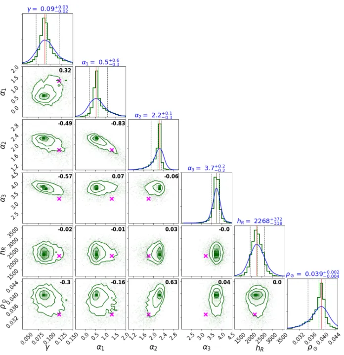
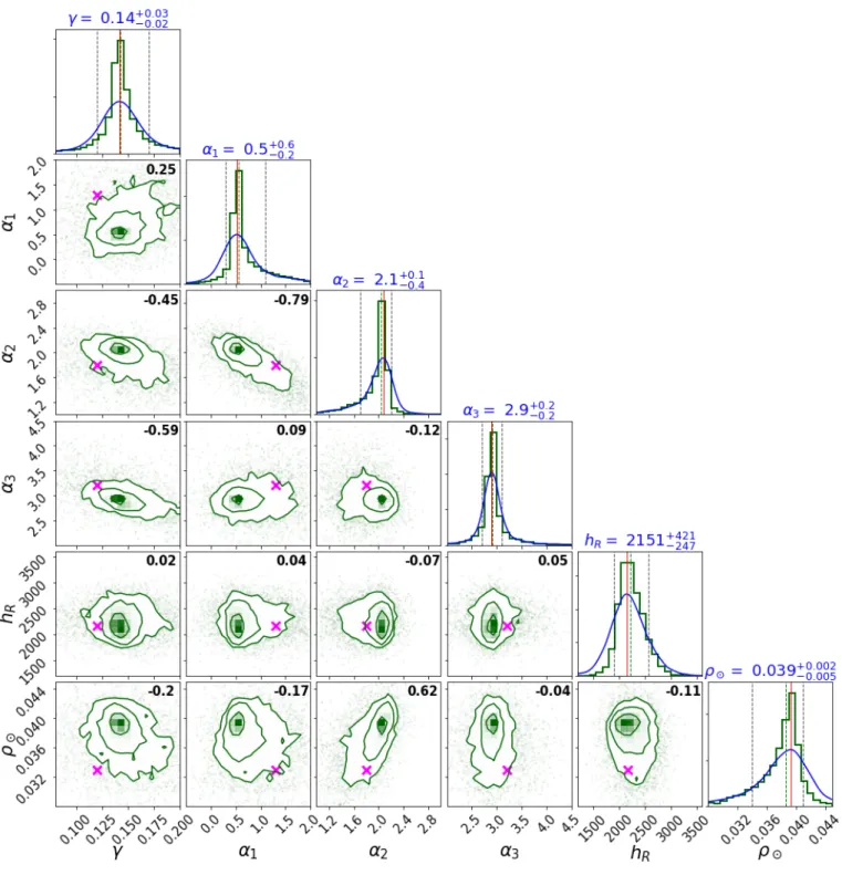
of α2 = 2.1+0.1−0.3in the mass range between 0.5 M and 1.53 M . The results of the slope at the high-mass range are trustable up to
4 M and highly dependent on the choice of extinction map (obtaining α3 = 2.9+0.2−0.2and α3 = 3.7+0.2−0.2, respectively, for two different
extinction maps). Systematic uncertainties coming from model assumptions are not included.
Conclusions.The good performance of BGM FASt demonstrates that it is a very valuable tool to perform multi-parameter inference using Gaia data releases.
Key words. Galaxy: fundamental parameters – solar neighborhood – Galaxy: stellar content – stars: formation – methods: analytical – methods: statistical
1. Introduction
Recently, the astrophysics community has successfully carried out important ground-based and space missions generating very large data sets. Large sky surveys with photometric and astro-metric data, such as Gaia data release 2 (Gaia Collaboration 2018), among others, represent a challenge for Galaxy modelling in terms of both the new types of data and the large amounts of data created. At the same time, new statistical techniques are having a significant effect on modern astronomy. The use of Bayesian statistics for the exploration of large parameter spaces, together with Monte Carlo Markov chains (MCMC) or approx-imate Bayesian computation (ABC), among others, are in rapid development.
Several attempts have been done to generate fast Milky Way simulations (e.g. Girardi et al. 2005; Juri´c et al. 2008;
Sharma et al. 2011orPasetto et al. 2016). It is demonstrated that the Galaxy models fromSharma et al.(2011) andPasetto et al.
(2016) can be used to explore large parameters spaces under machine-learning algorithms, MCMC, and ABC (e.g.
Rybizki & Just 2015;Pasetto et al. 2016). The Galaxia code is
able to work in two different modes: it can simulate the Milky Way from a Galaxy model based onRobin et al.(2003), or from N-body simulations. The fast performance of Galaxia relies on its sampling technique and its clever strategy adopted to avoid the simulation of unnecessary stars. The strategy ofPasetto et al.
(2016) to perform fast simulations of the Milky Way is based on the use of distribution functions. It constructs colour-magnitude diagrams (CMDs) of single stellar populations from N-body simulations, with low computational cost (Pasetto et al. 2012).
The Besançon Galaxy Model (BGM; Robin et al. 2003) is also a stellar population synthesis model for the Milky Way. It is a very powerful and versatile tool for the statistical analysis of the structure and evolution of the Milky Way. Moreover, it is a valuable tool for the preparation and validation of catalogues for space- and ground-based observational instruments and surveys. Recently, BGM was used to study the kinematics of the local disc from the RAVE survey and the Gaia first data release (DR1;
Robin et al. 2017), to evaluate the evolution of the Milky Way’s disc shape over time (Amôres et al. 2017), to constrain Galac-tic and stellar physics (Lagarde et al. 2017), to constrain the local initial-mass function (IMF) using Galactic Cepheids and
Tycho-2 data (Mor et al. 2017), and to study microlensing events in the Galactic bulge (Awiphan et al. 2016). Furthermore, BGM has also been useful, together with other Milky Way models, to study the bulge bar (Simion et al. 2017) and for the validation of the Gaia DR1 (Arenou et al. 2017). Nowadays, a BGM standard (BGM Std) simulation (e.g.Czekaj et al. 2014) has a computa-tional cost that is not adapted to exploring large parameter spaces using modern Bayesian iterative methods that require a very large number of simulations. To overcome this handicap we have developed a theoretical framework to generate very fast Milky Way approximate simulations based on BGM. This framework allows us to explore, among others, the parameter spaces of the IMF, the star formation history (SFH), and the density laws using ABC. The flexibility of the strategy presented here allows for the generation of fast approximate simulations for different Milky Way components, such as thin disc, thick disc, halo, and bulge. Our full strategy is codified to run on Apache Spark1 (Zaharia et al. 2012) and Apache Hadoop2, which are engines coming from business science suited to deal with large surveys. Thanks to its codification, BGM FASt is implemented in the big data infrastructure known as Gaia Data Analytics Framework (GDAF, e.g.Tapiador et al. 2017). As a first application of this complex strategy we use ABC algorithms, BGM, and Tycho-2 data to constrain the IMF, the local SFH, the local stellar mass density, and the thin-disc density laws.
In Sect.2we describe the BGM, and in Sect.3 we present the framework to generate the BGM fast approximate simula-tions (BGM FASt). In Sect.4we describe the treatment of the local dynamical statistical equilibrium in the context of BGM FASt. In Sect.5 we briefly describe the approximate Bayesian computation technique applied to explore the parameter space of the fundamental functions of the Milky Way. In Sect. 6 we present an evaluation of the BGM FASt performance in the solar neighbourhood. Results are presented in Sect.7while a discus-sion and concludiscus-sions are presented in Sects.8and9.
2. The Besançon Galaxy Model
In the present paper we use the following versions of the Galactic components of BGM chosen from a compromise between recent and stable updates.
For the stellar halo component we use the model from
Robin et al. (2014) and for the bulge-bar region we use the model described inRobin et al.(2012). For the thick disc com-ponent we use the model from the best fit obtained inRobin et al.
(2014) which is a thick disc with two main star-formation episodes at 10 and 12 Gyr. For the thin disc component we use the model described inCzekaj et al.(2014) with the updates on the parameters introduced inMor et al.(2017). The local dynam-ical statistdynam-ical equilibrium of BGM is ensured by dynamdynam-ical con-straints based onBienaymé et al.(1987). The last dynamics and kinematics updates fromBienaymé et al.(2015) andRobin et al.
(2017) are not considered in the present paper and will be incor-porated in the near future.
2.1. BGM star-generation strategy
The BGM has two main working modes to compute the genera-tion of the stars in the Galaxy. The tradigenera-tional approach relies on using a precomputed Hess diagram (Robin et al. 2003), while the more updated approach is able to generate the stars from a given
1 https://spark.apache.org/ 2 http://hadoop.apache.org/
set of fundamental functions (e.g. IMF, SFH, age-metallicity among others), making them evolve using a desired set of stel-lar evolutionary models (Czekaj et al. 2014). For each Galactic component we can choose whether we want to simulate it using the Hess diagram or the updated strategy. Alternatively, from the updated star-generation strategy we can build a Hess diagram from a given set of fundamental functions, and ingest it into BGM code afterwards to be used in a traditional way.
In this section we summarise the stellar generation strat-egy described inCzekaj et al.(2014), henceforth referred to as our standard strategy. Initially this strategy was developed for the thin-disc component but nowadays it can be used for other Galactic components.
In the BGM Std strategy, to generate stars born τ years ago for a given Galactic i-component (e.g. thin disc, thick disc, halo and bulge-bar), we start from a given total surface mass density at the position of the Sun (Σi ). We then use the SFH (ψi (τ)) to
distribute the surface mass density along τ as follows: Σi (τ) ≈Σ i ·ψ i (τ). (1)
For simplicity, the current version neglects the radial migra-tion. We setup the model so that the stars are born in the plane. We then redistribute them in the process of secular evolution by using the surface-to-volume mass density ratio at the position of the Sun (H (τ, ¯x )= Σ (τ)/ρ (τ)) to compute the volume stellar
mass density fromΣi , as follows
ρi(τ, x , y , z )= Σi (τ) Hi(τ, x , y , z ) = Σi ·ψi (τ) Hi(τ, x , y , z ) , (2)
where we have expressed the position ¯x in Cartesian Galactic coordinates as (x, y, z). The volume mass density is distributed throughout the Galaxy as
ρi(τ, x, y, z)= ρi(τ, x , y , z ) · Ri(τ, x, y, z), (3)
where Ri(τ, x, y, z) are the density laws for the given i-component
and Ri(τ, x , y , z ) = 1. We can then write Hi(τ, x , y , z ) as
the integral of the density law along the vertical direction at the position of the Sun:
Hi(τ, x , y , z )= Σi (τ) ρi(τ, x , y , z ) =Z ∀z Ri(τ, x , y , z) dz. (4)
Finally, from Eqs. (2)–(4), we can write the distribution of the volume mass density along position and age as follows
ρi(τ, ¯x)=
Σi ·ψi (τ)
Hi(τ)
· Ri(τ, ¯x), (5)
where for simplicity we call Hi(τ) to Hi(τ, x , y , z ). As
explained inCzekaj et al.(2014), the IMF distributes this mass density in three mass ranges. The star generation process goes through all the volume elements in the Galaxy. First, in a given volume element, for a given age sub-population the age of the star is drawn uniformly within the age limits. Afterwards, the mass of the star is drawn from the IMF. Next, the metal-licity is assigned depending on the age and position of the stars. In the most updated versions, the α-elements-to-iron abun-dance ([α/Fe]) is assigned to each star with a given probability (Lagarde et al. 2017). The evolutionary stage is then assigned to the star by interpolating the stellar evolutionary tracks. In a fol-lowing step, the process assigns to the generated star a given probability to be the primary component of a stellar multiple
system. This probability is assigned following the guidelines of
Arenou(2011). Finally, if the star is flagged as a primary compo-nent of a stellar multiple system, the standard strategy generates a secondary star with a mass drawn from the probability distri-butions described inArenou(2011).
For consideration in the following sections we define a BGM Std simulation to be one that works using the standard stellar generation strategy or a fixed Hess diagram built from the stan-dard stellar generation strategy.
2.2. Standard thin disc component
The thin disc component is described inCzekaj et al.(2014). The stars are generated as described in Sect.2.1. The thin disc popu-lation is divided in seven age sub-popupopu-lations. Usually the cho-sen age intervals are those described inBienaymé et al.(1987) but for the two youngest populations we use the age limits described inMor et al.(2017). The density distribution of each sub-population of the thin disc is assumed to follow an Einasto density profile as described inRobin et al.(2012), except for the youngest sub-population which follows the expression described in Robin et al. (2003). These profiles are characterised by the eccentricities of the ellipsoid (i.e. the axis ratio), the radial scale length of the disc (hR), and the radial scale length of the
disc hole (hRh). A velocity dispersion as a function of age is
adopted and the dynamical statistical equilibrium is ensured by using the strategy described in Bienaymé et al. (1987). Stellar evolutionary tracks and model atmosphere, combined with an age-metallicity relation, allow us to go from masses, ages, and metallicities to the space of the observables. In this process a three-dimensional (3D) interstellar extinction map is adopted.
3. Framework for the Besançon Galaxy Model Fast Approximate Simulation
A BGM Std simulation has a computational cost of ∼432 h of CPU time for a simulation of 106 stars, excluding the use of iterative methods like ABC or MCMC to explore large param-eter spaces. Hence, we have developed a new method, called BGM FASt, which is able to robustly simulate the Galaxy with a computational cost of ∼240 s of CPU time for a simulation of 106 stars. Thanks to the use of Apache Hadoop and Apache Spark environments (Zaharia et al. 2012) the computational cost should not scale with the number of stars as is the case in stan-dard environments (Julbe, priv. comm.).
3.1. The BGM FASt concept
The BGM FASt is a population-synthesis simulation of the Milky Way, obtained from a clever modification of a BGM Std simulation. The BGM FASt development is based on the dis-tribution function of the generated stars (Di). The Di carries
on the information about the generation of the stars in the i-component of the Galaxy (e.g. thin disc, thick disc, halo, bulge-bar) throughout the life of the given component up to the present day. This distribution function contains the chemo-dynamical information that is classically expressed by fundamental func-tions such as the IMF, the SFH, density distribution, the age-metallicity relation, and the radial age-metallicity gradient, among others. The Diis defined in a N dimensional space (¶i) for each
of the i-components of the Galaxy. This N dimensional space contains all the parameters that can be involved in a distribution function of the generated stars in the Galaxy. Let us introduce
the parameter space as follows:
¶i≡τ × M × Z × ¯x × ¯v × ¯p, (6)
where τ is the present age of the stellar object, M and Z are its initial mass and metallicity, and ¯x and ¯v are position and velocity, respectively. ¯p accounts for other independent parameters that, for some specific purposes, would be interesting to have explic-itly introduced in the distribution function. The α-elements-to-iron abundance ratio ([α/Fe]) is an example of one of the possible ¯p parameters and we treat this in the following section.
The strategy to generate a BGM FASt begins with the choice of a specific Mother Simulation with an imposed set of funda-mental functions. We use Mother Simulation to refer to a BGM Std simulation used as a seed to generate a BGM FASt simu-lation. This Mother Simulation is used as a main constituent to generate one or several BGM FASt simulations with different assumptions for the fundamental functions. The idea behind the BGM FASt strategy is that the number of stars generated in a given interval of the parameter space (Ni(Ʀ)) is proportional
to the mass dedicated to generate stars for that given interval (Mi(Ʀ)):
Ni(∆¶) ∝ Mi(∆¶), (7)
where∆¶ ≡ (∆τ, ∆M, ∆Z, ∆ ¯x, ∆¯v, ∆ ¯p). Equation (7) is valid for both the Mother Simulation and the BGM FASt simulation. If∆¶ is small enough, we can write a proportion between the number of stars and the masses relating both the Mother Simulation and the BGM FASt simulation:
NFASt i (∆¶) NMSt i (∆¶) ∝M FASt i (∆¶) MMSt i (∆¶) · (8)
Then we can approximate the number of stars for a given interval for a BGM FASt simulation as follows:
NiFASt(∆¶) ≈ M FASt i (∆¶) MMSt i (∆¶) · NiMSt(∆¶). (9)
Let us call weight to the mass ratio of Eq. (9): wi= MFASt i (∆τ, ∆M, ∆Z, ∆ ¯x, ∆¯v, ∆ ¯p) MMSt i (∆τ, ∆M, ∆Z, ∆ ¯x, ∆¯v, ∆ ¯p) , (10)
where we compute the mass dedicated to generate stars, in a given interval, from the distribution function of the generated stars that we present in following sections.
In practice, we generate a BGM FASt simulation by apply-ing a weight to each star of the Mother Simulation. This is done according to the parameters of the star, such as mass, age, posi-tion, and distance, among others. Thus, the resulting simulation is an approximation of the BGM Std simulation that would be obtained with the standard BGM star generation process.
We present the theoretical framework and the practi-cal implementation for the generation of a BGM FASt as follows.
First, in Sect.3.2, we describe the distribution function of the generated stars Di in the most generic context and its relation
with the masses involved in Eq. (10). This allows us to intro-duce the classical fundamental functions, such as the IMF and the SFH, and functions describing more complex scenarios. In a following step we consider a set of assumptions and approxima-tions to reach a Di function compatible with the Di implicitly
Next, in Sect.3.3, we discuss the treatment of stellar multiple systems as modelled in a BGM. We introduce the probability of obtaining a binary system at birth in our approximated Di. The
obtained expressions are useful for both the process ensuring the local dynamical statistical equilibrium and the computation of the surface mass stellar density at the position of the Sun. Finally after describing a generalizable weight expression, in Sect.3.4, we constrain it to the BGM context including stellar multiple systems.
3.2. The distribution function of the generated stars 3.2.1. Generic context and fundamental functions
In this section we describe the distribution function of the gen-erated stars in its most generic context. Under the given defini-tion of the parameter space (¶i) we can precisely define some
of the parameters belonging to ¯p. It is convenient for future purposes to write the distribution function Di(τ, M, Z, ¯x, ¯v, ¯p)
accounting explicitly for the ratio [α/Fe]. Subsequently, [α/Fe] is considered as one of the ¯p parameters and we can write Di(τ, M, Z, ¯x, ¯v, [α/Fe], ¯p0) in the N dimensional
space:
¶i≡τ × M × Z × ¯x × ¯v × ¯p = τ × M × Z × ¯x × ¯v × [α/Fe] × ¯p0. (11)
In our line of action, for the moment, we are interested in explic-itly representing age, mass, metallicity, position, velocity, and the ratio [α/Fe] in the distribution function. Subsequently we marginalize Di(τ, M, Z, ¯x, ¯v, [α/Fe], ¯p0) over the rest of the ¯p0
parameters: Gi(τ, M, Z, ¯x, ¯v, [α/Fe])= Z ∀ ¯p0∈ ¶i, Di(τ, M, Z, ¯x, ¯v, [α/Fe], ¯p0) d ¯p0, (12) where Gi is the distribution function of the generated stars for
the i-component in the reduced space ¶i r:
¶ir≡τ × M × Z × ¯x × ¯v × [α/Fe]. (13)
For simplicity let us henceforth refer to [α/Fe] using only α. The Gi(τ, M, Z, ¯x, ¯v, α) distribution function is such that the
integral over all the parameters that belong to the parameter space is the total number of generated stars in the i-component of the Galaxy:
Z
∀τ,M, ¯Z, ¯x,¯v,α ∈ ¶i r
Gi(τ, M, Z, ¯x, ¯v, α) dτ dM dZ d ¯x d¯v dα= Ni, (14)
and if we multiply by the mass before the integration, we have the total mass of the generated stars for the i-component of the Galaxy:
Z
∀τ,M, ¯Z, ¯x,¯v,α ∈ ¶i r
Gi(τ, M, Z, ¯x, ¯v, α)· M dτ dM dZ d ¯x d¯v dα= Mi. (15)
The mass of Eq. (7) can then be expressed as the integral of the distribution function for a given interval in the parameter space (∆¶i r): Mi(∆τ, ∆M, ∆Z, ∆ ¯x, ∆¯v, ∆α) = Z ∀τ,M, ¯Z, ¯x,¯v,α ∈ ∆¶i r Gi(τ, M, Z, ¯x, ¯v, α) · M dτ dM dZ d ¯x d¯v dα, (16)
and we can write Eq. (10) as
wi= R ∆¶i r GFASt i (τ, M, Z, ¯x, ¯v, α) · M d¶r R ∆¶i r GMSti (τ, M, Z, ¯x, ¯v, α) · M d¶r , (17) where d¶r ≡ dτ dM dZ d ¯x d¯v dα.
The true Gi(τ, M, Z, ¯x, ¯v, α) distribution function is unknown,
but its marginalization over combinations of parameters results in deeply studied functions such as the IMF, the SFH, the age-metallicity relation, the radial age-metallicity gradient, and also func-tions carrying information about the density distribution of the Galaxy or dynamical and chemo-dynamical information. Let us exemplify mathematically how some of these fundamental func-tions can be treated related to the distribution function.
The marginalization over the parameters τ, Z, ¯x, ¯v and α within the values that belong to the ¶i
rspace can be written as:
Z
∀τ,Z, ¯x,¯v,α ∈ ¶i r
Gi(τ, M, Z, ¯x, ¯v, α) dτ dZ d ¯x d¯v dα= ξi(M), (18)
where ξi(M) is the composite IMF for each one of the
i-components. Marginalizing now the Giover M, Z, ¯x, ¯v, α within
the values that belong to the ¶irspace we have the τ distribution of the generated stars that can be interpreted as the SFH of the whole i-component:
Z
∀ M,Z, ¯x,¯v,α ∈ ¶i r
Gi(τ, M, Z, ¯x, ¯v, α) dM dZ d ¯x d¯v dα= Ψi(τ). (19)
If we are interested in studying how the τ distribution depends on the position, we can then perform a marginalization over M, Z, ¯v and α, obtaining
Z
∀ M,Z,¯v,α ∈ ¶i r
Gi(τ, M, Z, ¯x, ¯v, α) dM dZ d¯v dα= fi(τ, ¯x). (20)
If in Eq. (20) we set ¯x = ¯x , the position of the Sun, then the
resulting function can be interpreted as the SFH at the position of the Sun.
The functions involving metallicity, such as the age-metallicity relation or the radial age-metallicity gradient, could also be considered in BGM FASt. If we marginalize Gi(τ, M, Z, ¯x, ¯v, α) over mass, α, and phase-space we get the Z distribution of stars formed τ years ago:
Z
∀ M, ¯x,¯v,α ∈ ¶i r
Gi(τ, M, Z, ¯x, ¯v, α) dM d ¯x d¯v dα= χi(τ, Z). (21)
The radial metallicity gradient can be deduced from a more complex expression obtained marginalizing Giover age, mass,
velocity and α: Z
∀τ,M,¯v,α ∈ ¶i r
Gi(τ, M, Z, ¯x, ¯v, α) dτ dM d¯v dα= ηi(Z, ¯x). (22)
This latter expression is the position and metallicity distribution of the generated stars throughout the life of the i-component.
Finally, information about chemo-dynamics and kinematics can be introduced with the following two equations.
Z ∀ M, ¯x, α ∈ ¶i r Gi(τ, M, Z, ¯x, ¯v, α) dM d ¯x dα= Qi(τ, Z, ¯v), (23) Z ∀ M,Z, α ∈ ¶i r Gi(τ, M, Z, ¯x, ¯v, α) dM dZ dα= Ki(τ, ¯x, ¯v). (24)
The spatial distribution of the volume mass density ( ρi g( ¯x))
that has been dedicated to generating stars for the Galactic i-component throughout its life can be written as follows
ρi g( ¯x)= Z ∀τ,M, ¯Z,¯v,α ∈ ¶i r Gi(τ, M, Z, ¯x, ¯v, α) · M dτ dM dZ d¯v dα. (25)
In the following steps it is useful to have the equation of the mass density dedicated to generating stars born τ years ago in a position ¯x: ρi g(τ, ¯x)= Z ∀ M, ¯Z,¯v ∈ ¶i r Gi(τ, M, Z, ¯x, ¯v, α) · M dM d ¯Zd¯v dα. (26)
Until now, we have described the distribution function of the generated stars in the Galaxy in a generic context. We have emphasised that our strategy can be generalizable and any of the fundamental equations described above (Eqs. (18)–(24)) can be used if we are able to write an analytical expression for them. 3.2.2. The approximate solution
In this section we find an approximation to the distribution func-tion of the generated stars compatible with BGM. At the same time this approximation aims to be extensible to other models of the Galaxy that use similar star-generation strategies. As the exploration of the velocity spaces is not included in the present paper, for simplicity we do not consider the kinematic part here. Our goal is therefore to find an approximate solution to the inte-gralR∀ ¯v ∈ ¶i
r
Gi(τ, M, Z, ¯x, ¯v, α) d¯v.
In this context the first assumption comes from a traditional strategy (e.g.Tinsley 1980), assuming that mass and age distri-butions are separated. Splitting the mass function from the func-tion of τ and ¯x as follows
ξi(M) · Fi(τ, ¯x). (27)
Moreover, the BGM assumes a metallicity distribution that depends on position and age. We can therefore introduce, in the equations, the probability that a star of a given age in a given position has a metallicity Z: Pi(Z|τ, ¯x). Furthermore, BGM
has recently included the possibility to use [α/Fe], a parame-ter which affects the stellar evolutionary tracks (Lagarde et al. 2017), assuming, from observational surveys, a certain probabil-ity that a given star has a given [α/Fe]. In general, for a given i-component, this probability depends on the age, the position, and the metallicity of the star and we denote it as Pi(α|τ, Z, ¯x).
From Eq. (27), and the metallicity and [α/Fe] distributions, we can write: Z ∀ ¯v ∈ ¶i r Gi(τ, M, Z, ¯x, ¯v, α) d¯v ≈ξi(M) · Fi(τ, ¯x) · Pi(Z|τ, ¯x) · Pi(α|τ, Z, ¯x), (28)
where the assumptions and approximations behind the math-ematical expression of the functions Fi(τ, ¯x), Pi(Z|τ, ¯x) and
P(α|τ, Z, ¯x) are imposed to be compatible with the BGM. Equa-tion (28) assumes, from the statistical point of view, that the probability to generate a star with mass M and the probability to generate a star τ years ago in a given position are conditionally independent. This means that the IMF is assumed to be indepen-dent of time and position.
The standard star-generation strategy described in Sect.2.1
guides us by using Eq. (5) to approximate the function Fi(τ, ¯x)
as follows Fi(τ, ¯x) ≈Σ i ·ψi (τ) Hi(τ) · Ri(τ, ¯x), (29) whereΣi
is the stellar surface mass density (∗/pc2) of the
gener-ated stars at the position of the Sun for the Galactic i-component, Hi(τ) is the surface-to-volume-density ratio at the position of the Sun, Ri(τ, ¯x) is the density distribution, and ψi is the SFH in the
solar neighbourhood.
Taking into account the approximations implicitly or explic-itly adopted in standard BGM we present a solid solution for the following integral Z ∀ ¯v ∈ ¶i r Gi(τ, M, Z, ¯x, ¯v, α) d¯v ≈ Σ i ·ψi (τ) Hi(τ) · Ri(τ, ¯x) · ξi(M) · Pi(Z|τ, ¯x) · Pi(α|τ, Z, ¯x), (30) where the IMF is normalized as R∀ M ∈ ¶i
rξ(M) · M dM = 1, the SFH in the solar neighbourhood is normalized as R
∀τ ∈ Πrψ (τ) dτ= 1, and by definition Pi(Z|τ, ¯x) and Pi(α|τ, Z, ¯x) are normalized to 1. Ri(τ, ¯x) and Hi(τ) are such that the integral
over the whole parameter space of Gi(τ, M, Z, ¯x, ¯v, α) gives the
total number of generated stars in the Galactic i-component. For simplicity, as BGM Std does, we assume an axi-symmetric structure with no radial migration. Additionally, we assume that for a given volume element, dρdt ≈ 0, where ρ is the stellar volume mass density. These assumptions allow us to use the density distributions (Ri(τ, ¯x)) described inRobin et al.
(2003) andRobin et al.(2014), derived to match the present den-sity distribution of each Galactic i-component.
3.3. Handling of the stellar multiple systems
The probability of obtaining a multiple system at birth in a star formation event is unknown, very complex, and can depend on many parameters, such as the metallicity, the mass of the molec-ular cloud, the turbulence, mass segregation, mass competition, and mass accretion rate (e.g.Bonnell et al. 2007;Kroupa et al. 2013). For these reasons, the BGM approach (e.g.Czekaj et al. 2014;Robin et al. 2012) is performed adopting an empirical law to match the observed present distribution function of multiple stellar systems (Arenou 2011). This approach assigns a certain probability to a generated star of being the primary component of a multiple system, depending on its mass and its luminosity class. Inside our framework this means a dependence on mass, age, and, through the stellar evolutionary models, Z and α. This probability is therefore P(bin|τ, M, Z, α).
Let us refer to the generated star susceptible to be flagged as either the single star or primary component of the binary sys-tem as the “primal star”. Once a primal star is decided as being a
primary component of a multiple system, a secondary star is gen-erated with a mass m. The mass m of the secondary is assigned following a probability distribution function (PDF) that depends mainly on the mass M and the luminosity class of the primary component, leading to P(m|τ, M, Z, α).
We introduce the stellar multiple systems in BGM FASt by simplifying their treatment under two assumptions: (1) The masses of primal stars (singles and primaries) are drawn from the IMF while the mass of the secondary follows the empirical laws described above, and (2) the age of the primary star follows the SFH, while the age of the secondary is assumed to be the same as the primary (i.e. both components were born together). With these two assumptions, the multiple stellar systems can be introduced in our analytical approach at low computational cost. We can compute first, at the position of the Sun, the surface mass density of secondary stars (Σi,$ ) as a function of the surface mass density of the primal stars (Σi,4 ) and afterwards computeΣi,4 as a function ofΣi . We begin by expressingΣi as Σi = Σ i,4 + Σ i,$ . (31)
Subsequently, the stellar volume mass density of primary stars at the position of the sun for the i-component is given by ρi,4 g ( ¯x ) ≈ Z ∀τ,M, Z, α ∈ ¶i r Σi,4 ·ψi (τ) Hi(τ) · R(τ, ¯x ) · ξi(M) · M · Pi(Z|τ, ¯x ) · Pi(α|τ, Z, ¯x ) dτ dM dZ dα, (32)
and the stellar volume mass density of secondary stars at the position of the sun for the i-component is given by
ρi,$ g ( ¯x ) ≈ Z ∀τ,M, Z, α, ∈ ¶i r mmax Z mmin Σi,4 ·ψi (τ) Hi(τ) · R(τ, ¯x ) · ξi(M) · Pi(Z|τ, ¯x ) · Pi(α|τ, Z, ¯x ) · P(bin|τ, M, Z, α) · P(m|τ, M, Z, α) m dm dτ dM dZ dα. (33)
We also want to compute the surface mass density; then, if we leave out Hi from the integrand of Eq. (33), we get the surface
mass density of secondary stars at the position of the Sun:
Σi,$ ≈Σ i,4 Z ∀τ,M, Z, α ∈ ¶i r mmax Z mmin ψi (τ) · ξi(M) · Pi(Z|τ, ¯x ) · Pi(α|τ, Z, ¯x ) · P(bin|τ, M, Z, α) · P(m|τ, M, Z, α) · m dm dτ dM dZ dα. (34)
Finally,Σi,4 is computed fromΣi
using Eqs. (31) and (34).
This result is very useful for both determining the weight function when considering multiple stellar systems as imple-mented in BGM (Sect.3.4) and computing the local dynamical statistical equilibrium (Sect. 4). In Sect. 4 we also particular-ize the computation ofΣi,4 when specifically using the thin disc component as described inCzekaj et al.(2014).
3.4. The weight
The strategy developed in previous sections allows us to give the analytical expression to compute the weights. These weights are able to transform the distribution of stars in the Mother Simu-lation, linked to a given set of Galactic fundamental functions,
into the distribution of the stars linked to other Galactic funda-mental functions adopted for a BGM FASt simulation. From (17) and (30) we obtain an expression for the weights applicable to Galaxy models that sample the stars from a distribution function of the form of Eq. (28), considering the assumptions discussed in Sect.3: wi(τ, M, Z, ¯x, α) ≈ R ∆¶i r Σi,FAS t ·ψi,FAS t HFASt i (τ) · RFASti (τ, ¯x) R ∆¶i r Σi,MS t ·ψi,MS t HMSt i (τ) · RMSt i (τ, ¯x) ·ξ FASt i (M) · M · P FASt i (Z|τ, ¯x) · P FASt i (α|τ, Z, ¯x) · d¶r ξMSt i (M) · M · P MSt i (Z|τ, ¯x) · P MSt i (α|τ, Z, ¯x) · d¶r · (35)
In the BGM context, including multiple stellar systems and taking into account the scenario described in Sect. 3.3, the weight that we apply in practice to generate a BGM FASt simu-lation is the following
wi(τ, M, Z, ¯x, α) ≈ R ∆¶i r Σi,4,FAS t ·ψi,FAS t HFASt i (τ) · RFASti (τ, ¯x) R ∆¶i r Σi,4,MS t ·ψi,MS t HMSt i (τ) · RMSt i (τ, ¯x) ·ξ FASt i (M) · M · P FASt i (Z|τ, ¯x) · P FASt i (α|τ, Z, ¯x) · d¶r ξMSt i (M) · M · P MSt i (Z|τ, ¯x) · P MSt i (α|τ, Z, ¯x) · d¶r , (36)
where we have substitutedΣi withΣi,4 from Eq. (35).
In our approach, the stellar evolutionary tracks are the same for both the Mother Simulation and the BGM FASt simulation. For simplicity, the probabilities Pi(Z|τ, ¯x) and Pi(α|τ, Z, ¯x) are
imposed and we are not going to explore them; they are equal for both the Mother Simulation and the BGM FASt simulation and we can marginalize the numerator and denominator over Z and α to obtain the final expression for the weights:
wi(τ, M, ¯x) ≈ R ∆τ, ∆M,∆ ¯x Σi,4,FAS t ·ψi,FAS t HFASt i (τ) · RFASti (τ, ¯x) R ∆τ,∆M,∆ ¯x Σi,4,MS t ·ψi,MS t HMSt i (τ) · RMSti (τ, ¯x) ·ξ FASt i (M) · M · dτ dM d ¯x ξMSt i (M) · M · dτ dM d ¯x . (37)
In practice, the weight in Eq. (37) is applied to each single star and each stellar system. This means that both the primary and the secondary components of the stellar system are weighted with the same value, according to the parameters of the primary component. We choose this way to apply the weights because in BGM Std the mass and age of the secondary star are drawn according to the mass and the age of the primary star. This choice ensures that the mass and age distributions of the primal stars in a BGM FASt simulation follow the pertinent IMF and SFH, and that the mass distribution of the secondary stars follows the empirical distributions described inArenou(2011).
The choice of the intervals for the integrals must be discussed for each particular case. Generally they must be small enough to preserve Eqs. (8) and (9). For tests and cases presented in the present paper, the choice of the mass interval is set to be very small (0.025 M ). For a given star of age τ we set the limits
of the integral to be the age limits of the age sub-populations to which the star belongs. Finally, as the BGM Std generation strategy assigns the density of its centre to the whole volume element, in BGM FASt we do not need to perform a volume element integral.
4. Local dynamical statistical equilibrium (LDSE)
By local dynamical statistical equilibrium we understand that, at the position of the Sun, the mass density distribution and the potential satisfy both the Poisson equation and the first-order moment of the collisionless Boltzmann equation for the vertical direction (Bienaymé et al. 1987). In this approach we consider axi-symmetry to solve both equations. To solve the first-order moment of the collisionless Boltzmann equation in the verti-cal direction, we also assume steady state, isothermal state, and decoupled radial and vertical motions. One possible methodol-ogy to ensure the LDSE is described inCzekaj et al.(2014) and summarised in Sect.4.1. As it requires a computational time that is not affordable for the methodology presented in this paper, we develop here analytical (Sect.4.2) and approximate (Sect.4.4) methods that ensure LSDE, significantly reducing the computa-tional cost.
4.1. Full LDSE
The iterative strategy described inCzekaj et al.(2014) performs, for a given set of Galactic fundamental functions, a local nor-malization and a sphere simulation around the Sun to compute at the position of the Sun: the surface mass density of the gener-ated stars,Σ , the volume mass density of the stars generated τ
years ago, that is ρg(τ, ¯x ), and the volume mass density for stars
generated τ years ago which are not stellar remnants at present, that is ρ(τ, ¯x )3. We define the stars which are not remnant at
present as those with τ ≤ Tlim(M, Z, α), where Tlim(M, Z, α) is
the maximum age that a star of a given mass, metallicity, and [α/Fe] reaches without becoming a remnant object. The stellar mass density at the position of the Sun is fitted with the stars that are not remnants at present and the white dwarfs’ density is added separately. The mass lost by the stars during their evolu-tion and the interacevolu-tion between components of a stellar multi-ple system are neglected. The total mass in stars, plus that of the interstellar medium, the dark matter, and the central mass, allows us to compute the radial force. At this stage, the dark matter den-sity distribution and the central mass is adjusted such that the model rotation curve fits the observations, the fit is done using the least-squares method in velocity. Finally, the Poisson and the first-order moment of the collisionless Boltzmann equation in the vertical direction are iteratively solved. The whole strategy is iterated from the beginning until convergence is reached. 4.2. Analytical LDSE
In this analytical approach to ensure LDSE, we follow the pro-cess described in Sect.4.1, but instead of using a simulation of a sphere around the Sun, we analytically derive the surface mass density of the generated stars (Σ ), the volume mass density of
the stars generated τ years ago (ρg(τ, ¯x )), and the volume mass
density for stars generated τ years ago which are not remnant at present (ρ(τ, ¯x )). As this approach concerns only the thin-disc
component, from now on we avoid the use of the index i. Using Eq. (31) we can expressΣ as the sum of the
sur-face density for primal stars (Σ4 ) and the surface density for secondary stars (Σ$ ). In an equivalent way, the ρg(τ, ¯x ) for the
generated stars can be expressed as
ρg(τ, ¯x )= ρ4g(τ, ¯x )+ ρ$g(τ, ¯x ), (38)
3 We note that the equivalent nomenclature for ρ
g(τ, ¯x ) and ρ(τ, ¯x ) in
Czekaj et al.(2014) is ρall (i) and ρ
obs (i).
and the stellar volume mass density of the stars with τ ≤ Tlim(M, Z, α) can be expressed as
ρ(τ, ¯x )= ρ4(τ, ¯x )+ ρ$(τ, ¯x ). (39)
Now we want to derive the stellar volume mass density of the primal stars at the position of the Sun ρ4
g(τ, Z, ¯x , α). Therefore,
from equation (32) we obtain ρ4 g(τ, Z, ¯x , α) ≈ Z ∀ M ∈ ¶r Σ4 ·ψ (τ) H (τ) ·ξ(M) · M · P(Z|τ, ¯x ) · P(α|τ, Z, ¯x ) dM. (40)
At this stage we assume that at the position of the Sun all the stars have solar metallicity Z = Z and for the moment BGM
assumes that the α-elements-to-iron abundance for the thin disc is α= α . The probabilities for Z and α then become
P(Z|τ, ¯x ) (1, if Z= Z 0, otherwise, (41) and P(α|τ, Z, ¯x ) (1, if α= α 0, otherwise. (42)
Combining Eqs. (40)–(42) we can approximate ρ4
g(τ, ¯x ) by ρ4 g(τ, ¯x ) ≈ Z ∀ M ∈ ¶r Σ4 ·ψ (τ) H (τ) ·ξ(M) · M dM. (43)
As mentioned above, the fit with the observational value of the volume stellar mass density at the position of the Sun is done with the stars with τ ≤ Tlim(M, Z, α). Therefore, as a next step,
we need to derive an analytical expression for the density of non-remnant primal stars at the position of the Sun. This is given by ρ4(τ, Z, ¯x , α) ≈ Z ∀ M ∈ ¶r O(τ, M, Z, α) ·Σ 4 ·ψ (τ) H (τ) ·ξ(M) · M · P(Z|τ, ¯x ) · P(α|τ, Z, ¯x )dM, (44)
where the function O(τ, M, Z, α) discussed in Sect.4.3is defined as
O(τ, M, Z, α)=(0, τ > Tlim(M, Z, α) 1, τ ≤ Tlim(M, Z, α)
. (45)
As before, we assume all the stars at the position of the Sun have Z= Z and α= α (Eqs. (41) and (42)), thus
ρ4(τ, ¯x ) ≈ Z ∀ M ∈ ¶r O(τ, M, Z , α )· Σ4 ·ψ (τ) H (τ) ·ξ(M)·M·dM. (46) Up to now we have derived analytical expressions for the volume densities of the primal stars ((43) and (46)). To complete Eqs. (38) and (39) we need to derive the analytical expressions for the mass density of secondary components. Considering Eq. (33) we can write ρ$g(τ, Z, ¯x , α):
ρ$ g(τ, Z, ¯x , α) ≈ Z ∀ M∈ ¶i r mmax Z mmin Σ4 ·ψ (τ) H (τ) ·ξ(M) · P(Z|τ, ¯x ) · P(α|τ, Z, ¯x ) · P(bin|τ, M, Z, α) · P(m|τ, M, Z, α) · m dm dM. (47)
Next, to continue reducing computational time, we assume that the mass of the secondary is only dependent on the mass of the primary component P(m|τ, M, Z, α) ≈ P(m|M) and we consider this probability is uniform and given by
p(m|M) ≈ 1 M−Mmin, if Mmin< m ≤ M 0, otherwise , (48)
where Mminis the minimum mass needed to generate a star. This
expression states that the mass of the secondary star is always equal or less massive than the corresponding primary compo-nent.
We introduce a second approximation assuming that for a given generated primal star the probability of being the primary component of a multiple system is given by
P(bin|τ, M, Z, α) ≈(0, τ > Tlim P(bin|M), 0 < τ ≤ Tlim
. (49)
This probability, as defined, is not null only for the non-remnant stars. Therefore, using Eq. (45), it can also be expressed as p(bin|τ, M, Z, α)= O(τ, M, Z, α)·p(bin|M). In other words, this approach assumes that the probability of being a primary compo-nent of a binary system is null for those stars which are remnant at present. Introducing Eqs. (48) and (49) in (47), we have ρ$ g(τ, Z, ¯x , α) ≈ Z ∀ M∈ ¶i r mmax Z mmin O(τ, M, Z , α ) · Σ4 ·ψ (τ) H (τ) ·ξ(M) · P(Z|τ, ¯x ) · P(α|τ, Z, ¯x ) · P(bin|M) · P(m|M) · m dm dM. (50)
The above assumptions imply that secondary stars are never rem-nants, thus ρ$(τ, Z, ¯x
, α) = ρ$g(τ, Z, ¯x , α).
As done for primal stars, we assume that all the stars at the position of the Sun have solar metallicity Z = Z and α = α .
Therefore, ρ$(τ, ¯x )= ρ$g(τ, ¯x ) ≈ M=Mmax Z M=Mmin m=Mmax Z m=Mmin O(τ, M, Z , α ) ·Σ 4 ·ψ (τ) H (τ) ·ξ(M) · P(bin|M) · P(m|M) · m dm dM. (51) As done for primal stars, we leave out H (τ) from (51) to reach the expression forΣ$ :
Σ$ ≈ τ=τend Z τ=0 M=Mmax Z M=Mmin m=Mmax Z m=Mmin O(τ, M, Z , α ) ·Σ4 ·ψ (τ) · ξ(M) · P(bin|M) · P(m|M) · m dm dM dτ. (52)
At this point we have on hand all the analytical expressions to compute theΣ that fits the observed stellar mass density at
the position of the Sun (ρ obs) for the thin disc stars with τ ≤ Tlim(M, Z, α). To do so we use Eqs. (51) and (46) in (39) and
set ρ(τ, ¯x ) = ρ obs, with ρ obs being the observed stellar mass
volume density at the position of the Sun for stars which are not remnant at present. We then solve the resulting equation forΣ4 and computeΣ from (31) and (52).
For the practical implementation of the analytical approach developed in this section we adopt Mmin = 0.09 M and Mmax=
120 M , the mass range of the evolutionary models we are using
at present (Chabrier & Baraffe 1997;Bertelli et al. 2008,2009). For p(bin|M) in Eq. (49) we follow the expression for main sequence stars inArenou(2011).
4.3. The non-remnant fraction (Ω)
The O function (45) is directly related with the stellar evolution-ary tracks considered through the expressions of Tlim(M, Z, α).
We define Tlim(M, Z, α) as the maximum age for which a star of
a given mass, metallicity, and α-elements-to-iron abundance is still not a stellar remnant. As discussed in the previous section, for the O function we consider solar metallicity Z= Z and solar
α = α . We use, for the moment, the stellar evolutionary tracks
Bertelli et al.(2008) andChabrier & Baraffe(1997) considered in Czekaj et al. (2014) which do not consider the α-element abundance; therefore Tlim(M, Z, α)= Tlim(M, Z). From the
men-tioned stellar evolutionary tracks we derive Tlim(M, Z ) fitting
three truncated logarithmic expressions to the two-dimensional (2D) grid of mass and age limit for Z= Z . We end up with the
following expressions for M/M ≥ 7. Tlim(M, Z ) ≈ exp(−1.6 · ln(M)+ 20.8) (53) for 2.2 < M/M < 7.0, Tlim(M, Z ) ≈ exp(−2.7 · ln(M)+ 23.0) (54) for 2.0 < M/M < 2.2, Tlim(M, Z ) ≈ exp(−2.7 · ln(2.2)+ 23.0) (55) for M/M ≤ 2.2, Tlim(M, Z ) ≈ exp(−3.5 · ln(M)+ 23.3). (56)
With these latter expressions we have everything we need for the execution of the analytical LDSE as described in Sect.
4.2. At this point, to take into account that the BGM Std strat-egy samples the age of the stars uniformly inside each age sub-population (see Sect.2.2) we substitute the O function by theΩ function in the equations of Sect.4.2. TheΩ(τ, M, Z ) function
is defined as Ω(τ, M, Z )= 1, Tlim(M, Z ) > Tendj (τ) Tlim(M,Z )−Tinij(τ) Tendj (τ)−Tinij(τ) , T j ini(τ) ≤ Tlim(M, Z ) ≤ T j end(τ) 0, Tlim(M, Z ) < T j ini(τ), (57) where Tinij (τ) and Tendj (τ) are respectively the low and high age boundaries for each of the seven age sub-populations of the thin disc ( j = 1 . . . 7). We note that Tinij (τ) and Tendj (τ) obviously depend on τ, because the age τ of the star establishes the j-sub-population to which the star belongs. We emphasise that theΩ function defined above gives the fraction of stars which are not remnant at present and is constant with τ inside the limits of each age sub-population. Furthermore, when defining O andΩ functions we are neglecting both the entangled evolution of stars belonging to the multiple stellar systems and the mass lost by the star during its evolution. If in the future we want to imple-ment the effect of the mass lost by the stars during its evolution, we can do this by introducing a new function, L(τ, M, Z, α), into the equations, accounting for the fraction of mass that a given star has lost during its evolution up to the present time. If at
some point we are interested in accounting for the entangled evolution of a stellar multiple system then we need to imple-ment the desired evolutionary model of stellar systems directly in the BGM Std strategy, generate a Mother Simulation, and finally modify Tlimaccordingly.
4.4. Approximate LDSE
In Sects. 4.2 and 4.3 we explained how, in the full process to ensure the LDSE (Sect. 4.1), we can substitute the entire simulation of a sphere around the Sun by crafted analytical expressions which are computationally undemanding. Here we complete the construction of an approximate LDSE strategy by complementing Sects. 4.2 and 4.3 with a final assumption to make the process even faster. As described in Sect.4.1 in the full LDSE process, the central mass and the dark matter density distribution is adjusted such that the model rotation curve fits the observations. We can avoid the computational cost of this adjustment by assuming that the central mass density and the dark matter density distribution are invariant under variations of the Galactic fundamental functions4.
We now test the performance of the approximate LDSE to evaluate the assumptions that we made and to constrain its range of validity. In the following section we present a set of tests com-paring the results obtained when applying the full LDSE process against the results of our approximate LDSE.
4.5. Validation of the approximate LDSE
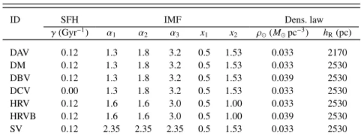
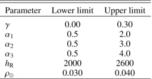
We develop three tests to evaluate the goodness of our approx-imate method (Sects. 4.2–4.4). These tests quantify the di ffer-ences, when using the approximate instead of full method, in some of the key parameters resulting from the LDSE process. All the tests are performed using the seven model variants described inMor et al.(2017) that were built with different assumptions of the IMF, the SFH, and the density laws. In Table1we present their main parameters. These model variants cover the range of parameters that we want to explore in this paper well, and there-fore they are a good set to perform the tests. The parameters for the thin disc density laws which are not listed in Table 1 are adopted to be the same as used inMor et al.(2017), being the functional forms of the density laws listed inRobin et al.(2003). The rest of the model ingredients which are not specifically indicated in Table 1, for example the atmosphere models, the stellar evolutionary tracks, the age-metallicity relation, and the age-velocity dispersion, are adopted to be the same as in “Model B” listed in Table 5 ofCzekaj et al.(2014).
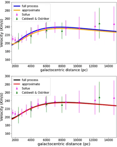
In the first test we show that our approximate method obtains a rotation curve compatible with the one resulting from the full method. For all model variants, we obtain differences of less than 2% in the rotational velocity between a galactocen-tric radius from 3 kpc to 14 kpc. Moreover these differences are much smaller than discrepancies between the observational val-ues (e.g.Caldwell & Ostriker 1981andSofue 2015). In Fig.1
we present the results for the two model variants where we found the highest discrepancies between the rotation curve obtained from both methods. The discrepancies along the curve from 3 kpc to 14 kpc are always smaller than 5 km s−1. Thus we
con-sider that the approximated LDSE is valid within these galacto-centric radii.
4 In practice we impose that the central mass density and the dark
mat-ter density distribution take the values of the Default Model Variant in
Mor et al.(2017).
Table 1. Parameters for the SFH, the IMF and the density laws of the seven model variants adopted fromMor et al.(2017).
ID SFH IMF Dens. law
γ (Gyr−1) α 1 α2 α3 x1 x2 ρ (M pc−3) hR(pc) DAV 0.12 1.3 1.8 3.2 0.5 1.53 0.033 2170 DM 0.12 1.3 1.8 3.2 0.5 1.53 0.033 2530 DBV 0.12 1.3 1.8 3.2 0.5 1.53 0.039 2530 DCV 0.00 1.3 1.8 3.2 0.5 1.53 0.033 2530 HRV 0.12 1.6 1.6 3.0 0.5 1.00 0.033 2530 HRVB 0.12 1.6 1.6 3.0 0.5 1.00 0.039 2530 SV 0.12 2.35 2.35 2.35 0.5 1.53 0.033 2530
Notes. We show: (1) the three slopes of the initial mass function (α1,α2
and α3) and the two mass limits (x1and x2) between the three truncated
power laws of a Kroupa-like type; (2) the stellar volume mass density at the position of the Sun ( ρ ); and (3) the radial scale length of the old
thin disc (hR).
The second test compares for each model variant the eccen-tricities of the Einasto density profiles which are fitted inside the process that ensures the LDSE. The Einasto eccentricities are computed for each one of the seven age sub-populations of the thin disc. In all cases we find differences smaller than 0.7%.
Our third test compares the local volume stellar mass density of all the thin-disc age sub-populations. For each model variant we check our capability to recover the density values of Table 1 ofMor et al.(2017). The discrepancies are within the error bars and are always smaller than 5%.
We want to point out that these tests are the first empirical demonstration that our strategy for the BGM FASt simulation is well founded. Whereas it is true that they validate the equations behind the weight function, they do not evaluate the capabilities of the weight function itself to generate a BGM FASt simula-tion. To do so we need to directly test distributions of observ-able parameters obtained with BGM FASt simulations. Tests on age and mass distribution are also needed to deeper validate the BGM FASt strategy. These tests are presented in Sect. 6 and AppendixA.1.
5. ABC to infer Galactic fundamental functions
5.1. The ABC method
For very complex models such as the BGM, to obtain the exact likelihood function is mathematically impossible or com-putationally prohibitive. In these cases the ABC algorithms allow us to compute an approximate posterior PDF of the explored parameters. In this paper we use a sequential Monte Carlo approximate Bayesian computation algorithm (SMC-ABC) because of its balance between high acceptance rate and independence of the outcomes. The algorithm that we use is fur-ther described inJennings & Madigan (2017), and is available as a python package named astroABC. The SMC-ABC method is an improvement of basic ABC acceptance-rejection sampling (ABC) to optimise the acceptance rate. The basic ARS-ABC contains the theoretical bases of the SMC-ARS-ABC algorithm. This latter first generates a proposed set of parameters ¯θ from the prior PDF. Subsequently, the algorithm generates the simu-lated data using the proposed set of parameters in a given model, and finally the set of parameters is accepted as part of the pos-terior PDF if the simulated data (Dsimu) are equal to the real
data (D); otherwise ¯θ is rejected and we start the process again. This algorithm is very restrictive because it is almost impossi-ble to find a model with a given set of parameters that perfectly
Fig. 1. Two examples of the comparison between the rotation curve obtained with both the full process to ensure LDSE and the rotation curve obtained with the approximate LDSE. Top panel: results for the DAV variant fromMor et al.(2017). Bottom panel: results for the HRBV variant from Mor et al.(2017). The green triangles show the data points derived from theCaldwell & Ostriker(1981) rotation curve assuming R0= 8000 pc and V0= 230 km s−1for the Sun. The magenta
triangles show the data points of the rotation curve fromSofue(2015). For Sofue data, error bars are provided by the author, while we have estimated the errors of the data fromCaldwell & Ostriker(1981) fol-lowing the expressions and tables in their paper.
reproduces the data. Usually one uses the ARS-ABC, relaxing the condition Dsimu = D and approximating the method as
follows
(1) Generate ¯θ from the prior PDF.
(2) Simulate data Dsimfrom the model M with parameters ¯θ.
(3) Calculate the distance δ(D, Dsim) between D and Dsim.
(4) Accept ¯θ if δ is smaller than a given threshold (υ) δ ≤ υ; return to 1.
This approximate algorithm needs to adopt an adequate distance metric δ and a threshold υ. When υ → 0, the algorithm is sam-pling exactly from the posterior PDF. Very small values of υ diminish the acceptance rate of the algorithm, and therefore the choice of υ must be a compromise between computational cost and accuracy of the posterior PDF. We want to emphasise that ARS-ABC samplers generate independent outcomes; each itera-tion is independent from the previous.
Other ABC methods, like the so-called free likelihood MCMC samplers (MCMC-ABC), are also built to optimise the acceptance rate. The MCMC-ABC increases the acceptance rate by modifying MCMC sampling algorithms (such as Metropolis-Hastings) to be able to work without the need of the likelihood (Marjoram et al. 2003), but the price paid in this case is that the outcomes are dependent (Marjoram et al. 2003). In a different way, the SMC-ABC improves the acceptance rate with a double
entangled optimisation. For each iteration, the algorithm uses kernels to assign a higher sampling probability to the sets of parameters with better results. The resulting new sampling prob-ability is used in the next iteration. In other words, regions of the parameter space with better results are visited more frequently. The application of kernels in the limits of the prior PDF can sometimes produce a posterior PDF slightly wider than the limits stated by the prior PDF. The use of the kernels is complemented with an adaptive threshold υ, where the upper and lower limits have to be set. This allows to go from a more relaxed threshold in the first iterations down to a small threshold for the last ones, optimising the sampling of the posterior PDF in terms of com-putational time. We emphasise that for a given expression for the distance metric and a given υ, the outcomes are still independent in the SMC-ABC.
Now we need to choose the data in accordance with the parameters that we want to infer. Observations can only pro-vide a small subset of all the potential data defining the Milky Way system. This limitation forces us to search for summary statistics, which are of a lower dimension and are incomplete. If the chosen summary statistics, S, are statistically sufficient for D then the posterior PDF under the summary data P(θ|S) is equivalent to the posterior PDF under the full data P(θ|D). In practice it is very difficult, or impossible, to formally iden-tify rigorous summary statistics sufficient for D. As suggested in
Marjoram et al.(2003) we use a more heuristic approach for our specific problem. In the following section we propose summary statistics S that capture information on the ¯θ essential parame-ters of the Milky Way. Once sufficient statistics are established, D is replaced by S in the algorithm as done inMarjoram et al.
(2003). The theoretical basis for these algorithms can be found inMarin et al.(2011),Beaumont et al.(2009) andSisson & Fan
(2010), for example.
5.2. Bayesian inference in the solar neighbourhood
For the appropriate use of the ABC algorithm described above, we need to define, for each of the specific scientific goals that we want to achieve, our sufficient statistics S, a distance met-ric δ, and a threshold υ. For both the evaluation of the BGM FASt performance (Sect.6) and the science demonstration cases (Sect.7), we consider as our sufficient statistics S the star counts in a binned four-dimensional space of position, apparent mag-nitude, and observed colour. This means that for the purposes of this paper we define our sufficient statistics as the number of stars in each bin of latitude, longitude, visual Tycho mag-nitude (VT), and Tycho-2 colour (B − V)T. Specifically, our S
is the colour-magnitude diagram split in three latitude ranges: (|b| < 10), (10 < |b| < 30), and (30 < |b| < 90). We choose the bin size of the colour-magnitude diagram to be large enough to allow for a robust statistical analysis to be performed, but small enough to avoid loosing information. As mentioned in the previous section, our choice of S is based on our previous experience when comparing BGM with observational data. We know that the observed colour-magnitude diagrams in different regions of the sky offer very valuable information to constrain the IMF, the SFH, the local stellar mass density, and the density laws (e.g.Mor et al. 2017;Robin et al. 2014,2012). In some of these papers these colour-magnitude diagrams have already been used as sufficient statistics combined with ABC algorithms (e.g.
Robin et al. 2014). Furthermore, inCzekaj et al. (2014) it was demonstrated that the division of the sky into the three above-mentioned latitude ranges is very useful to analyse the Galactic fundamental functions by fitting BGM to Tycho-2 data. In our
star counts analysis we always work inside the completeness limits of the observational catalogues and therefore our sufficient statistics when using Tycho-2 data are limited at VT = 11 where
Tycho-2 is complete up to 99%.
Once our sufficient statistics are defined, we need to choose the distance metric to quantify differences between the observed and simulated data, δ (Sobs, Ssimu). We use this to compare the
simulated Ssimu and the observed Sobs data. For this paper
we use the following expression, which we call Poissonian distance: δP(Sobs, Ssimu)= N X i=1 qi·(1 − Ri+ ln(Ri)) , (58)
where Riis defined as the quotient Ri = fi/qiand qiand fi are
the number of stars in the data and the model, respectively. Addi-tionally, we penalise the cases where there are no stars observed in the bin but the model predicts stars to be present by replac-ing qiand fiin the formula with qi+ 1 and fi+ 1, respectively.
The defined distance metric becomes zero when the simulation and the observations have the same number of stars in each bin. The smaller the value of the distance metric, the closer Ssimu
is to Sobs. From Kendall & Stuart (1973) and Bienaymé et al.
(1987) we know this formula is a good choice for the compari-son between observed and simulated colour-magnitude diagrams in terms of star counts. Furthermore, in Mor et al. (2017) we already introduced the idea that expression (58) can be under-stood as a distance metric.
Finally, we choose an upper limit and a lower limit for the threshold υ by experimenting with different values to have a good balance between computational cost and accuracy of the posterior PDF.
6. Evaluating BGM FASt at the solar neighbourhood
In this section we evaluate the behaviour of BGM FASt in the solar neighbourhood and we demonstrate that the performance of the BGM FASt strategy is independent of the Mother Sim-ulation. In Sect. 6.1we use both BGM FASt and BGM Std to simulate the solar neighbourhood. We then analyse the resulting samples limited in apparent magnitude by comparing colour dis-tributions and CMDs. Additionally, we extend the comparison to mass and age distributions for a deeper analysis of the BGM FASt performance. We do these comparisons in the complete-ness regime of Tycho-2 catalogue, and therefore we use samples limited in Tycho visual apparent magnitude (VT) up to 11, where
Tycho-2 is complete at 99%.
In Sect.6.2we present a test for the BGM FASt framework together with the ABC algorithm, consisting in exploring the parameter space of the SFH, demonstrating that we are able to correctly recover an imposed SFH in the solar neighbourhood. 6.1. BGM FASt versus BGM Std
To evaluate the performance of the BGM FASt we compare sim-ulations generated with the same sets of fundamental functions obtained from both the BGM FASt and BGM Std strategy. We have selected five model variants fromMor et al.(2017): DAV, DBV, DCV, HRV and SV. All of them constitute a good frame-work to analyse the BGM FASt behaviour in the solar neighbour-hood as they adequately cover the parameter space that we want to explore with BGM FASt in Sect.7. For each model variant we perform the tests using both theDrimmel & Spergel(2001) and
Marshall et al.(2006) extinction maps5. The main set of compar-isons aims to evaluate the behaviour of BGM FASt when using as Mother Simulation the best fit variant fromMor et al.(2017) (the DAV variant) obtained using Galactic Cepheids and Tycho-2 data. The DAV variant is our choice for the Mother Simula-tion when exploring a six-dimensional (6D) parameter space in Sect.7.2. In the tests we evaluate the effects of changing one or more parameters of the fundamental functions when generating BGM FASt simulations according to the model variants DBV, DCV, HRV and SV.
Additionally we repeat the comparisons but use the DCV variant (constant SFH) as the Mother Simulation. These addi-tional tests help us to evaluate the BGM FASt performance in several aspects. First, they allow us to demonstrate whether or not the performance of the BGM FASt strategy is indepen-dent of the Mother Simulation. Second, we are able to anal-yse possible dependencies on the total number of stars of the Mother Simulation. Third, they allow us to study simultaneous changes of the IMF and the SFH. Finally, they provide us with more data, which can be used to better interpret the obtained results.
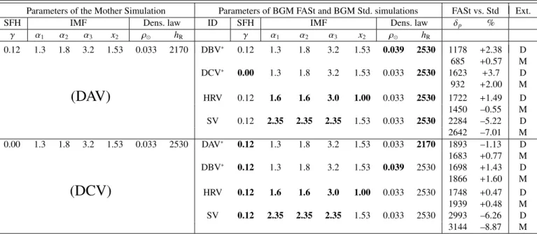
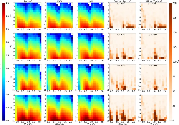
In Table 2 we summarise the parameters of the IMF, the SFH, and the density laws for the variants involved in the tests. The functional form for the SFH is assumed to be an exponen-tial law, the IMF is assumed to be a three-times-truncated power law and the density profiles are assumed to be of Einasto shape. In the first column we show the parameters that we use for the Mother Simulation: the DAV and DCV. In the second column we show the parameters for the BGM FASt simulations. The same parameters are also used to perform BGM Std simulations. We mark in bold text the parameters that have been modified from the Mother Simulation to generate the BGM FASt simulation. In the third column (FASt vs. Std) we present a summary of the global results comparing BGM FASt with BGM Std simu-lations, δp is for the Poissonian distance from Eq. (58) and %
refers to the discrepancies of the total number of stars between BGM FASt and BGM Std simulations, that is ((# Stars in BGM FASt – # Stars in BGM Std)/# Stars in BGM Std) ∗100. We note that for all cases except the SV variant the discrepancies in the total number of stars is smaller than 4%. When looking to the Poissonian distance metric we note that all the values are below 2000, except, again, for the SV variant. The Poissonian distance between BGM FASt and BGM Std simulations is one order of magnitude smaller than the difference between the best fit variant fromMor et al.(2017) and Tycho-2 data.
When comparing colour, age, and mass distributions between BGM FASt and BGM Std, for the cases of Table2, we note that in general the differences in relative counts per bin are smaller than 5% (see Figs. A.1–A.3, for details). In some cases, such as when using the IMF (SV variant) fromSalpeter
(1955) or when changing the mass limits of the IMF (HRV vari-ant), the difference in the youngest population of the thin disc and for the high mass range can reach about 10%. These di ffer-ences are also reflected in the colour distributions. We demon-strate in AppendixBthat these discrepancies (>10%) come from the sampling noise involved in the BGM Std generation strategy. Occasionally, mostly for flat values of the IMF at high masses, the mass distribution of the youngest massive stars is influ-enced by the distribution of sampling noise in very low-mass
5 The Marshall et al. (2006) extinction map covers the longitude
ranges −100 < l < 100 and the latitude ranges |b| < 10. Therefore, when simulating with the Marshall map we use the Drimmel map for the rest of the sky.
Table 2. Summary of the results of the BGM FASt vs. BGM Std tests and the parameters for the SFH, the IMF, and the density laws of the model variants.
Parameters of the Mother Simulation Parameters of BGM FASt and BGM Std. simulations FASt vs. Std Ext.
SFH IMF Dens. law ID SFH IMF Dens. law δp %
γ α1 α2 α3 x2 ρ hR γ α1 α2 α3 x2 ρ hR 0.12 1.3 1.8 3.2 1.53 0.033 2170 DBV∗ 0.12 1.3 1.8 3.2 1.53 0.039 2530 1178 +2.38 D 685 +0.57 M DCV∗ 0.00 1.3 1.8 3.2 1.53 0.033 2530 1623 +3.7 D 932 +2.00 M
(DAV)
HRV 0.12 1.6 1.6 3.0 1.00 0.033 2530 1722 +1.49 D 1450 –0.55 M SV 0.12 2.35 2.35 2.35 1.53 0.033 2530 2284 –5.22 D 2642 –7.01 M 0.00 1.3 1.8 3.2 1.53 0.033 2530 DAV∗ 0.12 1.3 1.8 3.2 1.53 0.033 2170 1893 –1.13 D 1683 +0.77 M DBV∗ 0.12 1.3 1.8 3.2 1.53 0.039 2530 1698 +1.43 D 1866 +1.60 M(DCV)
HRV 0.12 1.6 1.6 3.0 1.00 0.033 2530 1748 +0.47 D 1939 +0.48 M SV 0.12 2.35 2.35 2.35 1.53 0.033 2530 2993 –6.26 D 3144 –8.87 MNotes. x1= 0.5 for all the model variants. The units for this table are the same as in Table1. The variants marked with an asterisk are those which
are less affected by the sampling noise discussed in AppendixB. The final column indicates the assumed 3D extinction map in each case; it can beDrimmel & Spergel(2001) (D) orMarshall et al.(2006) (M).
reservoirs6. The sampling noise in very-low-mass reservoirs pro-duces, on average, more stars than predicted by the imposed dis-tribution function for the mass range between 1.53 M and 4 M .
From AppendixB, we deduce that we must use a Mother Sim-ulation such that the combination of the imposed fundamental function minimises the effects of the noise in the very small mass reservoir; this is the case of the DAV variant, for example.
After the analysis presented in this section and also in Sect. 4.5we conclude that BGM FASt is performing correctly in the solar neighbourhood.
6.2. Recovering an imposed SFH
To show that BGM FASt together with the ABC algorithm is capable of inferring a given parameter, we perform several tests trying to recover an imposed SFH of the thin disc. We assume the SFH to be a decreasing exponential function:
ψ = Kψ· eγτ, (59)
where Kψ is the normalization constant, γ is the inverse of the characteristic timescale (e.g. Snaith et al. 20157) and τ is the time. The coordinate origin of the τ space is at present (τ = 0) and the values are positive in the direction backwards in time, to the past, until the age of the thin disc (in this case we impose τ = 10 Gyr). We use one BGM Std simulation, with an imposed value of γ, playing the role of the observations, and we use one BGM Std simulation, with an imposed γ, as a Mother Simulation to generate BGM FASt simulations while mapping the parameter space.
6 As described inCzekaj et al.(2014) Eq. (1) in each age bin, the mass
available to be spent on star production in a given volume element, is the mass reservoir.
7 We want to emphasise that we use different nomenclature from
Snaith et al.(2015).
We use Eq. (58) as a distance metric and the sufficient statis-tics S described in Sect.5.2. The threshold υ is set to be small enough to obtain statistically significant results. The simulations are covering the full sky with a limiting apparent magnitude of VT = 11 to mimic the completeness selection function of
Tycho-2. Moreover we added the Tycho-2 photometric errors to the simulated observables (Czekaj et al. 2014;Mor et al. 2017). The first test consists in using a BGM Std simulation with γ = 0.12 Gyr−1as the observational data and as the Mother
Sim-ulation. For the second test, we use a BGM Std simulation with γ = 0.12 Gyr−1as observational data and another BGM Std
sim-ulation with γ= 0.00 Gyr−1as the Mother Simulation. Our third
test consists in using a BGM Std simulation with γ= 0.00 Gyr−1 as observational data and another BGM Std simulation with γ = 0.12 Gyr−1 as the Mother Simulation, that is, the inverse
of the second test. We find that in the three tests presented here our strategy succeeded in recovering the imposed γ value with a narrow posterior PDF. The posterior probability distribution for the γ parameter resulting from the last test is plotted in Fig.2. In green we show the prior PDF while in red we plot the pos-terior PDF. It is interesting to see how from a given prior PDF we end up with a posterior PDF of a very different shape. This is expected as according to the Bayesian statistics theory, the bet-ter the information coming from the data, the smaller the depen-dency of the posterior PDF on the prior PDF.
7. BGM FASt science demonstration cases
To show the capabilities and the strength of BGM FASt sim-ulations, we present two science demonstration cases using Tycho-2 data. We want to prove that our BGM FASt strategy together with the ABC algorithm obtain consistent results by analysing data from the solar neighbourhood. The solar vicinity is a good region to start with, allowing comparisons with previ-ous results. In both cases we use Tycho-2 data with VT < 11. We