Design and testing of experimental free-piston cryogenic expander

Design and Testing of Experimental Free-Piston Cryogenic Expander

By

Ryan Edward Jones

B.S., Mechanical Engineering University of South Carolina, 1997

SUBMITTED TO THE DEPARTMENT OF MECHANICAL ENGINEERING IN PARTIAL FULFILLMENT OF THE REQUIREMENTS FOR THE DEGREE OF

MASTER OF SCIENCE IN MECHANICAL ENGINEERING

AT THE

MASSACHUSETTS INSTITUTE OF TECHNOLOGY FEBRUARY 1999

* 1999 Massachusetts Institute of Technology All rights reserved

Signature of Author ... . ... ... . I eartment of Meolnical Engineering January 31, 1999

Certified by ... ... ... .

/ Joseph L. Sr4dith, Jr.

Professor of Mechanical Engineering Thesis Supervisor

A ccepted by

...

.

Ain A. Sonin

Design and Testing of Experimental Free Piston Cryogenic Expander

By

Ryan Edward Jones

Submitted to the Department of Mechanical Engineering on January 31, 1999 in Partial Fulfillment of the Requirements for the Degree of Master of Science in

Mechanical Engineering

ABSTRACT

An experimental free piston cryogenic expander was designed and constructed as a part of a feasibility test. Unlike most cryogenic expanders, there were no physical connections for controlling or monitoring the position of the piston. Rather, a linear variable differential transformer (LVDT) was designed and constructed on the outside of the cylinder wall to non-intrusively monitor the piston's position. Signals

from the LVDT, pressure transducers and thermocouples were collected by a data acquisition system and integrated into a real-time control routine. The control routine digitally switched valves on the warm and cold ends of the expander to control the pressure-volume relation in the cold end of the expander.

Results from experimental testing were compared with theoretical thermodynamic and dynamic analysis of the single-stage apparatus to determine the expander's performance. Comparisons showed that the expander's behavior closely resembled the theoretical models, and identified design considerations and improvements for a second-generation expander. Although the expander was not insulated for thermal performance, significant cooling was evident under testing conditions.

Thesis Supervisor: Joseph L. Smith, Jr. Title: Professor of Mechanical Engineering

Acknowledgements

I would like to thank professor Smith for his patience and guidance throughout the project and for giving

me that extra kick when I needed it. I would like to thank professor Brisson who saved me on numerous occasions in the lab and loaned me vital equipment in exchange for my first born. I am also grateful to Mike and Bob who were always willing to help me and prevent shrapnel from flying around the shop. To my fellow C.E.L. students, thanks for all the sanity checks and comic relief.

I would like to say thank you to my family, who were forced to listen, and pay the phone bill, to all the

good and bad times I have endured. Their love and support have meant more than words can express. To my in-laws, thank you for all the pep talks and confidence you gave me. Most Importantly, I would like to say thank you to my wife, Catherine. Without her love, patience and understanding, I would never have made it. Thank you everyone!

The financial support for this research was provided by both the Starr Fellowship and professor Joseph Smith.

Table of Contents

A cknow ledgemnents ... 3

Table of Contents ... 4

Nom enclature ... 6

List of Figures and Tables...8

1 Introduction...11 1.1 Background...11 1.1.1 Expansion Engines...11 1.2 Project Objective...12 1.3 Expander Cycle... 13 1.4 Project Phases...15

1.4.1 M odeling and Optim ization...15

1.4.2 Fabrication and Assem bly ... 15

1.4.3 Instrum entation and Control... 15

1.4.4 Testing and Analysis...16

1.4.5 Results...16

2 Expander M odeling and Optim ization ... 17

2.1 Isentropic processes...17

2.2 Therm odynam ic m odeling...18

2.2.1 Rubber Geom etry ... 18

2.2.2 Fixed Geom etry...23

2.3 Optimization... 25

2.4 Dynamic Modeling... 27

3 Design of Free-Piston Expander...32

3.1 Apparatus Design ... 32

3.1.1 Valves...33

3.1.3 Brass Cap... 35

3.1.4 Piston... 37

3.2 Instrum entation and Signal Conditioning...38

3.2.1 Linear V ariable D ifferential Transform er ... 38

3.2.2 Pressure...41

3.2.3 Temperature... 41

3.3 Control D esign...41

4 Results...45

4.1 O ptim ization...45

4.1.1 Rubber G eom etry ... 45

4.1.2 Fixed Geometry ... 50 4.2 D ynam ics ... 54 4.3 Experim ental...55 4.3.1 Equilibrium ... 65 4.3.2 Speed... 67 4.3.3 Cooling... 69 5 Conclusion ... 70

A ppendix A : N orm alized Equations...71

A ppendix B : Single Equation Opitm ization... 77

A ppendix C : Calibration Curves for Instrum ents ... 80

A ppendix D : Q Basic control program ... 81

A ppendix E: D ata M anipulation W orksheet...86

A ppendix F: D ynam ic A nalysis W orksheet...91

Nomenclature

AE Change in Internal Energy of a System p Density of Working Fluid

: Viscosity of Working Fluid Ac :Cross-Sectional Area of Piston A0 Area of Orifice in Throttle Valve

A, :Surface Area of Piston

CP :Specific Heat Capacity at Constant Pressure C, :Specific Heat Capacity at Constant Volume dP Differential Pressure

ds Differential Entropy dT Differential Temperature dV Differential Volume

FC Force Acting on Piston in the Cold Region FS Force on Piston from Gas Spring in Warm Region FV Force Acting of Piston as a Result of Piston Motion

g Gravitational Acceleration

G Radial Clearance Between Piston and Cylinder Wall H Stroke Length

k Specific Heat Ratio m : Mass of Working Fluid m* :Normalized Mass M, :Mass of Piston

P Pressure

P* :Normalized Pressure

PA Intermediate Tank A Pressure PB Intermediate Tank B Pressure Pi. :Inlet Line Pressure

Pout :Exhaust Line Pressure Q Heat Transfer

R Universal Gas Constant

T Temperature

t :Time

To : Ambient Temperature T* Normalized Temperature Ti. :Inlet Line Temperature Tout :Exhaust Line Temperature

v Voltage

V Volume

V* :Normalized Volume

Vmax Maximum Volume of Cylinder

Vtank Volume of Intermediate Pressure Tank W Work Transfer

List of Figures and Tables

Figure 1: Schematic of Free-Piston Expander... 13

Figure 2: Ideal P-V Relation for Cold Region of Expander... 14

Figure 3: W arm Region M odel from State 1-+2...20

Figure 4: Cold Region M odel from state 4-+5 and 5-+6... 21

Figure 5: Subsystems for discharge process 5-+6... 22

Figure 6: W arm Region Charging Process 6-+7 and 7-+8 ... 23

Figure 7: Ideal P-V Relation for High Stroke ... 24

Figure 8: Ideal P-V Relation for Low Stroke ... 25

Figure 9: Free Body Diagram of Piston ... 27

Figure 10: Contour Integration for Inverse Laplace Transform ... 31

Figure 11: Detailed Sketch of Free-Piston Testing Apparatus... 32

Figure 12: Spool Valve Configurations...34

Figure 13: M achined Throttle Valves...35

Figure 14: W arm-End Assembly...36

Figure 15: Assembly Cross-Section View A-A ... 37

Figure 16: W arm End Sketch of Piston...38

Figure 17: Cross-Sectional View of LVDT... 39

Figure 18: LVDT Electrical Schematic...40

Figure 19: Flowchart for Automatic M ode ... 42

Figure 20: Logic to Determine Sates in Cycle ... 44

Figure 21:, P*eId -V(oid diagram for M atched Stroke ... 45

Figure 22:, T*coid -V*cod Diagram for M atched Stroke ... 46

Figure 23: Equilibrium Intermediate Pressures for Rubber Geometry Model...47

Figure 24: Optimized T*0u for Rubber Geometry M odel (P*oue=.1)... 48

Figure 25:, T*m.-V* ,, m Diagram for M atched Stroke ... 48

Figure 27: P*cold -V*cod Plot for Rubber Geometry Model with Four Pressure Tanks ... 50

Figure 28: Low Stroke Cycle for Fixed Geom etry M odel... 51

Figure 29: High Stroke Cycle for Fixed Geom etry M odel... 51

Figure 30: Low Stroke Optim ization...52

Figure 31: High Stroke Optim ization...53

Figure 32: Com bined Unm atched Optim ization Results ... 53

Figure 33: Blow -in Process with Only Viscous Dam pening... 54

Figure 34: Blow -in Process w ith Throttling effects ... 54

Figure 35: V *, aId vs. Tim e for Low Stroke ... ... . ... 56

Figure 36: P*, . vs. Tim e for Low Stroke...56

Figure 37: P*C0ld vs. Tim e for Low Stroke ... 56

Figure 38: P*coId vs. V * wd Plot for Low Stroke ... 58

Figure 39: P*,. vs. V*, . Plot for Low Stroke... 58

Figure 40: V *cold vs. Tim e for M atching Stroke ... 60

Figure 41: P*, , vs. Tim e for M atching Stroke... 60

Figure 42: P*.od vs. Tim e for M atching Stroke ... 60

Figure 43: P*coId vs. V *cod Plot for M atched Stroke... 61

Figure 44: P*w, vs. V *,. Plot for M atched Stroke... 61

Figure 45: V * ld vs. Tim e for High Stroke...62

Figure 46: P*, . vs. Tim e for High Stroke...63

Figure 47: P*,OId vs. Tim e for High Stroke ... 63

Figure 48: P*cOId vs. V 'c Plot for High Stroke... ... ... 64

Figure 49: P*,a vs. V *

,r

Figure 50: Steady-State Operating Conditions of the Expander (P*.ut = .2) ... 66

Figure 51: Experim ental D ynam ics of Blow-in Process ... 68

Figure 52: V *oId vs. Tim e for M axim um Cycle Speed ... 68

Figure 53: M inim um Experim ental Tem perature vs. Tim e (P*0,=.2)...69

Figure 55: Calibration for Linear Variable Differential Transform er... 80

Table 1: List of Parts for Figures 13-15 ... 34

Table 2: Options in M anual M ode...42

Table 3: V alve Control for States in Cylce ... 43

Table 4: U ser Options in Autom atic M ode ... 44

Table 5: W ork Results for Low Stroke...59

Table 6: W ork Results for M atched Stroke...62

Table 7: W ork Results for H igh Stroke...65

1 Introduction

1.1 Background

Cryogenic engineering utilizes low-temperature refrigeration processes for numerous research and practical applications. These areas range from studying material properties at extreme temperatures to commercial

manufacturing and bottling of gases. As in any industry, the need for these processes fuels the research into developing equipment and methods of obtaining cryogenic temperatures more efficiently and reliably. With improved designs and lower cost, cryogenic refrigerators will become an integral and necessary part of our technological society.

There are three common process used to obtain cryogenic temperatures: evaporation, isenthalpic expansion and isentropic expansion. Depending on the application and requirements of the system, cryogenic systems may incorporate any combination of these processes. This research project focused on the design and construction of a free-piston expander to isentropically cool the working fluid.

1.1.1 Expansion Engines

The first law of thermodynamics states that the change in internal energy of a system equals the net flow of energy across the system boundary. For a steady-state closed system, the first law of thermodynamics may be written in the form,

AE=Q - W

Eqt 1

where Q represents heat transfer into the system and W represents work done by the system. One can see that if work is removed from a system adiabatically, the intemal energy of the system must decrease. However, in an isentropic expansion, both the pressure and volume are changed simultaneously. To see the effect of an isentropic process, the second law of thermodynamics must be employed.

The second law of thermodynamics deals with the entropy of a system. Unlike energy, which is conserved, entropy may be generated in an isolated system. Depending on the rate of the processes and methods of heat transfer within a system, the change in entropy over time for an isolated system must be greater than or equal to zero. Although all processes realistically generate entropy, through careful design, the entropy generation can be

minimized such that the process can be modeled as reversible. For an adiabatic, reversible process involving an ideal gas, the second law of thermodynamics

k- 1

T 2

P2

T

Eqt 2

illustrates that the temperature ratio between states one and two is a function of the pressure ratio at those states. Since equation 2 is written for an ideal gas, k represents the specific heat ratio, C,/C,. This isentropic decrease in temperature was the basis for both the design and analysis of the free-piston expander.

The most general setup for an expansion engine involves a piston that is driven by an external motor. This general process begins by charging a region under a piston. The piston, which is attached to an external driving mechanism, expands the gas isentropically. Once the pressure in the expansion region reaches the exhaust line pressure, the exhaust valve opens and the piston sweeps the cooled gas out of the expander. The work transferred from the expanding gas is rejected to the driving mechanism through the piston. Although all expansion engines need some method of transferring energy in the form of work away from the cold region, it is not always necessary to have physical linkages to an external driver.

This project dealt with a free-piston design for an expansion engine, which involved expanding the gas similar to the method described above, but without a piston connected directly to an external driver. This free-piston design used a pressure differential across the piston to control its motion and extract work from the working fluid. Advantages of the free piston expander over contemporary expanders included fewer moving part, greater dependability and a system that could be sealed to prevent loss of the working fluid over time.

1.2 Project Objective

The objective of this project was to design and construct an experimental free-piston cryogenic expander. Since the free-piston expander was controlled and timed without physical connections, two particular aspects of the system's behavior needed to be investigated. First, could a free-piston expander be constructed and dynamically controlled reliably? Second, how closely would the thermodynamic behavior of the expander reflect the theoretical models developed for a single stage apparatus?

1.3 Expander Cycle

To begin a discussion on the expander, an overall description of the cycle is required. Shown in Figure 1, the system schematic illustrated a piston and cylinder arrangement attached to two intermediate pressure tanks, modeled as constant pressure reservoirs. For the purpose of discussion, tank A was at a higher pressure than tank B. These tanks were never in direct communication with each other. The working fluid, N2 gas, could only flow between the

tanks via the warm region of the expander. The Nitrogen, which passed into to or out of the warm region, passed through both a throttle valve and a 5-port, 2-way spool valve used to select the intermediate pressure tank that was connected to the warm end. 2-way valves were located on the inlet and exhaust ports in the cold region of the expander to control the gas flow.

5/2-Spool Valve

A

B

Pressure

Tanks

Throttle Valve

Warm region

Piston

PistonCylinder

Cold

region

I nI et Va lveO

Exhaust Valve

Figure 1: Schematic of Free-Piston Expander

In the actual system, the throttles and 5/2-spool valve were integrated into a warm end assembly that sealed the top of the cylinder. A complete discussion of the details of the system design will be reserved for chapter 3.

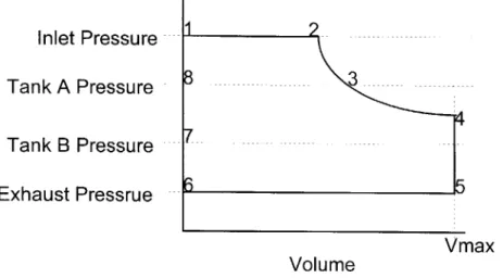
To understand the operation of the expander, consider the pressure verses volume plot illustrated in Figure 2. This P-V diagram represented the idealized cycle for the cold region of the expander. Just prior to state 8, the piston in Figure lwas resting on the bottom of the cylinder, and there was no working fluid in the cold region. Both the inlet and exhaust valves were closed, and the warm region was connected to tank A. When the pressure in the cylinder equaled the pressure in tank A, the inlet valve was opened and the pressure jumped to the inlet line pressure before there was any motion of the piston. This was the labeled state 1 in Figure 2. There was now a pressure differential across the piston, which induced motion. The piston moved upward rapidly until the pressure in the

warm region reached Pin and equilibrium was established. For the purpose of this explanation, the piston was assumed to have no mass and consequently, vibration was neglected.

Inlet Pressure

1

2

8

3

Tank A Pressure

7

4

Tank B Pressure

Exhaust Pressure

5

Cold End Volume

Figure 2: Ideal P-V Relation for Cold Region of Expander

There was now a pressure drop across the throttle valve since Pwan = Pin and PA<Pinl. As the compressed gas in the warm region was throttled into tank A, more high-pressure gas entered the cold region to maintain pressure equilibrium. This charging process continued until the volume in the cold region reached that of a preset value, denoted by V2. This preset value at state 2 was the only adjustable parameter in the actual system for a given inlet

and exhaust pressure. Once the system reached state 2, the inlet valve was closed and the isentropic expansion began.

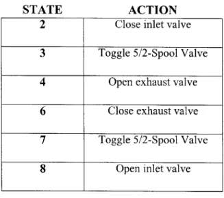
Immediately after the inlet valve was closed, the pressure in both the cold and warm region equaled the inlet line pressure. As the compressed gas in the warm region continued to be throttled into tank A, the pressure in the cylinder dropped. When the cylinder pressure equaled that of tank A, state 3, the 5/2-spool valve was toggled to allow more decompression into tank B. This continued expansion between states 3 and 4 was also isentropic, which resulted in an additional temperature drop. At state 4, it was assumed that the cylinder pressure reached that of tank B as the piston reached top dead center simultaneously. At this point, the exit valve was opened. The blow down process, state 4 to 5, was not accompanied by any motion of the piston because there was zero void space in the warm region at top dead center and there was no gas to expand. The piston began to sweep out the expanded gas in the cold region as gas from tank B flowed through the throttle valve to recharge the warm region. When the piston reached the bottom of the stroke, state 6, the exit valve was closed, allowing the pressure in the cylinder to increase

to that of tank B. At state 7, the 5/2-spool valve toggled back to tank A and gas continued to charge the cylinder through the throttle valve until the pressure in the cylinder equaled PA, at which time the cycle repeated.

1.4 Project Phases

To investigate the free-piston expander, the project was divided into four stages of development. The first stage was to develop models and optimization routines to analyze the performance of the expander. Next, the expander apparatus was designed and fabricated using an on-sight machine shop. With the apparatus physically constructed, the emphasis shifted to instrumentation and development of a control routine to automate the cycle. Finally, data was collected for analysis and compared with the optimized models.

1.4.1 Modeling and Optimization

To investigate the performance of the free-piston expander, thermodynamic analysis of the cycle was used to predict the temperature drop of the working fluid under various operating conditions. Concurrently with the modeling, optimization routines were developed to determine the optimum design parameters of the expander. Through these optimization routines, the stability and steady-state cyclic operating conditions of the system were also investigated.

1.4.2 Fabrication and Assembly

With the theoretical modeling complete, the design and fabrication process began. Many components of the expander, including the cylinder and cold-end actuators were from previous experiments. A critical component of the free piston design was the warm end assembly, which controlled the switching for the intermediate pressure expansions and dissipated the work as heat by throttling the compressed nitrogen in the warm-end of the cylinder. The piston and non-intrusive position sensing equipment were also integrated into the system. All components for the project were machined in an on-sight machine shop and assembled on an existing test stand.

1.4.3 Instrumentation and Control

A major concern of the free-piston expander, was the reliable control and data acquisition during the cycle.

To provide real-time control and feedback of the system's operation, data was continuously sampled and checked to

inside the cylinder. To acquire this information, a linear variable differential transformer (LVDT) was designed and integrated into the apparatus.

In addition to controlling the expander, data needed to be collected on the thermodynamic behavior of the system to compare with the theoretical models generated in stage 1 of the project. The control program collected data over several cycles and downloaded the information to floppy disks for manipulation.

1.4.4 Testing and Analysis

The final stage of the project consisted of testing the expander under various operating conditions. The different test setups were intended to provide information about the actual performance of the system and it's limitations, which identified design considerations for the second-generation expander. The raw data obtained from the experiments was imported into a data manipulation worksheet, which provided useful graphical results

illustrating the cycle's processes.

1.4.5 Results

2

Expander Modeling and Optimization

The first stage of the project was to create a thermodynamic model of the expander cycle and optimize the system's parameters for maximum cooling. Before the cycle model was developed, the property relations of an isentropic process were developed for an ideal gas. The next step involved developing the governing equations for the cycle processes and non-dimensionalizing the equations to provide a more general analysis. The equations were then entered into a worksheet and various system configurations were optimized. Finally, a dynamic model of the piston during the blow-in process was developed to investigate the system's dynamic response and vibration during rapid processes in the cycle.

2.1 Isentropic processes

It was established that adiabatic expansions of a system remove energy from the system. It was also shown that the second law provided a quantitative analysis of this cooling effect. This section was devoted to developing the isentropic relations upon which the thermodynamic model was developed.

To begin, entropy was defined as a function of temperature, T, and volume, V. Taking partial derivatives of the respective variables resulted in equation 3.

6s

S

ds=

dT+

-dV

6T

6V

Eqt3 Substituting the appropriate Maxwell relations and the constitutive relation for an ideal gas into equation 3, the differential pressure-volume relation for an ideal gas became equation 4.

dP

dV

C

--

+ C -- =0

Eqt 4 Integrating equation 4 and rearranging the variables, a relationship between the volume and pressure ratios during an isentropic process for a ideal gas resulted as shown in equation 5 for constant values of C, and C,.

P2QJ/TI

P i

V 2

Eqt 5

Substituting equation 5 into the work integral

W

outj

Eqt 6

and evaluating it from any state 1 to 2 resulted in the following.

P k-11

W out-

_k

V

Eqt 7

Equation 7 represented the maximum work attainable from an isentropic expansion. Although all of the energy was unattainable due to friction losses and irreversibilities, equation 7 provided a means by which to judge the

expander's performance.

2.2 Thermodynamic modeling

2.2.1 Rubber Geometry

In order to evaluate the cooling effect of the free-piston expansion cycle, a thermodynamic model of the system was developed. An evaluation of the cycle, which related both the warm and cold regions, resulted in a set of equations for the pressure, volume, mass and temperature of the system at each state. The First model that was developed involved "rubber geometry". This meant that during the final isentropic expansion, the piston always reached top dead center at the same instance that the pressure in the warm region equalized with the pressure tank B.

The rubber geometry model began by analyzing the process from state 8 to 1, the blow-in process. Unlike the ideal process in Figure 2, the model included a volume change associated with the sudden change in pressure.

Because this process occured very rapidly, the warm region of the expander was modeled as a closed system, which went through an isentropic compression. However, the cold region, which had zero volume at state 8, was modeled as an open system that expanded. The governing equations for both the warm and cold regions were as follows for the blow-in process.

Cold region:

m 1-C -Tl

_{i=-W outc + C P-T in-m i}

Eqt 8 Warm region: M -C -(T -T 8 ~ PdV=-W0outw -.8 Eqt 9 k- 1 k

T

_P

These equations combined with the ideal gas law and the fact that Wo",c=-Woutw, yielded the equilibrium equations for state 1.

The next process, from state 1 to 2, was the charging process. During this time, the cold region was modeled as an open system with constant pressure expansion. At state 2, the pressure was still equal to the inlet line pressure and the volume of the cold region was a preset parameter, denoted by the V2. A first law analysis of the

cold region, equation 11, only contained two unknowns, the temperature and mass at state 2.

m2' CvT 2

m C *Tl

P

1)+

C

*T

)

Eqt 11

Using the ideal gas law to relate the mass and temperature of the working fluid at state 2, the equation could be rearranged to solve for the equilibrium properties at state 2.

To solve for state 2 in the warm region, consider the system illustrated in Figure 3.

Warm Regi n

-M.V. 2

Cylinder

M.V.

1

Piston

Figure 3: Warm Region Model from State 1->2

The portion of gas contained in material volume 2 was throttled into tank A, and material volume 1 defined the gas that remained in the warm region of the cylinder. A second law analysis of material volume 1 revealed that the warm region temperature remained constant from state 1 to 2. Using this result and the ideal gas relation, it was shown that the mass ratio from state 1 to 2 equaled the volume ratio.

Recall that the inlet valve was closed at state 2, and the first isentropic expansion began. For this process, the cold region was modeled as a closed system that was governed by the following equations.

T 3 _'P3

ds=O=C -In --

- R-In

Eqt 12

ds=o=C p-In

+ C *n

3

V2

2

Eqt 13 In both equation 12 and 13, there was one unknown, which was solved for directly to determine all the properties in the cold region at state 3. To model the warm region during the process from state 2 to 3, a similar material volume approach as shown in Figure 3, was employed. In this situation, the same isentropic relations used for the cold region, were applied to the region labeled material volume 1 in Figure 3. All of the isentropic expansions

throughout the cycle were modeled in this same manner. Although the free-piston system was constructed to allow for two isentropic expansions, models, which were discussed in section 4.1.1, were developed for multiple tanks.

During the final isentropic expansion, the rubber geometry model assumed that the warm region volume decreased to zero simultaneously with the pressure differential across the throttle valve. Consequently, there was zero volume in the warm region and no movement from the piston when the pressure in the cold region suddenly dropped as the exhaust valve opened. However, there was a temperature drop associated with this sudden pressure drop in the cold region. To analyze the blow-down and discharge processes, consider the diagram shown in Figure 4.

M. V. (X) M. V. (Y)

Exhaust Line

Cnst. Pressure

Figure 4: Cold Region Model from state 4->5 and 5- 6

Similar to the warm-end material volume analysis during the isentropic expansions, the cold region was divided into two material volumes, shown in Figure 4. This illustration represented the system at state 4, where the sum of the volumes occupied by X and Y together equaled the maximum volume of the cylinder. Material volume X represented the mass that remained in the cylinder immediately after the blow-down process from state 4 to 5.

Material volume Y was the mass that was removed from the cold region during this process. For modeling purposes, there was an isentropic expansion of material volume X and a constant pressure expansion of material volume Y as it entered the exhaust line. The resulting first law analysis of the combined subsystems is shown in equation 14.

m x

-T

x

+

my

-T

y

)

-

m

-T

4]C

V=-P

_{out-V y5}

Eqt 14

Isentropic expansion relations were used to obtain all properties of material volume X at state 5. The ideal gas law was used to change the constant pressure work term to a mass and temperature relation for material volume Y. Finally, the mass of subsystem Y was eliminated by relating it to the mass at state 4 and subsystem X, which had been completely determined. The only unknown left was the temperature of control mass Y at state 5, which could

be solved for explicitly from equation 14. The cooling effect of the blow-down process was the first time the mass in the cold region became a factor. In all of the other processes, the temperature ratios were independent of the mass in the cold region of the expander.

The next process involved the discharge of the cooled gas and charging of the warm region with gas throttled in from the low-pressure intermediate tank. The cold region process was modeled as an open system, and a first law analysis showed that the work input to the system from the falling piston was used to exhaust the cooled gas. Consequently, there was no temperature change in the cold region from state 5 to 6. However, the two subsystems shown in Figure 4 were mixed in the exhaust line at state 6. A first law analysis of this process, equation 15, showed that the resulting final temperature, of the

(mx-My) T 6 mx5-Tx5+my5-T y5

Eqt 15 working fluid at state 6, was a mass weighted average of the two temperatures found in state 5.

To solve for the warm region properties at state 6, the set of subsystems shown in Figure 5 was analyzed. Subsystems labeled B and C were modeled as material volumes, while subsystem E was modeled as an open system. As before, all systems were assumed adiabatic, permitting only work and mass transfer. A

Throttle

M.V. C

Valve

M.V. B

Tank

B

E

Exhaust Line

Figure 5: Subsystems for discharge process 5->6

first law analysis of Figure 5 revealed that there was no temperature change in material volume C as it was throttled into the warm region. This was a result of zero void space in the warm region at state 5 and the modeling

assumption that all the fluid in the intermediate pressure tank was equaled to the ambient temperature. Once the expander system reached state 6, the exhaust valve was closed, and the piston remained at rest on the bottom of the cylinder from state 6 through state 8.

During this time, the working fluid in the intermediate tanks was used to pressurize the warm region of the expander. From state 6 to 7, gas from the low-pressure tank flowed through the throttle valve and into the warm region. Figure 6 illustrated how this process was modeled.

M.V. B

Intermediate

Pressure Tank

Throttle

Valve

Y

Pisto

Figure 6: Warm Region Charging Process 6->7 and 7--8

Subsystem B was a constant pressure material volume that compressed the mass of subsystem X into control volume Y.

Again, a first law analysis combined with the ideal gas law and conservation of mass resulted in an explicit equation for the temperature of the warm region at state 7. At this time in the cycle, the pressure in the cylinder equaled that of the low-pressure intermediate tank and the volume of the warm region equaled Vmn,. By toggling the 5/2-spool valve, the next intermediate tank began to charge the pressure in the cylinder.

The process from state 7 to 8 was analyzed in the same manner. Recall that this system only consisted of two intermediate pressure tanks, but this analysis could easily be adapted to multiple intermediate pressure tanks.

Once the cylinder was completely charged to PA, the cycle began again. The state equations obtained from this analysis were then used to program the optimization routines, which are discussed later.

2.2.2 Fixed Geometry

The rubber geometry analysis assumed that the system processes matched at state 4. This meant that the piston reached top dead center simultaneously with the cylinder pressure equalizing with the low-pressure intermediate tank. In reality, the size of the cylinder was fixed, and depending on the relation between V2 and PB,

understand the behavior of the free-piston expander, fixed geometry models were developed in a similar manner to the rubber geometry model.

The first case considered was when the piston reached top dead center prior to the pressure in the warm region dropping to that of the low-pressure intermediate tank. Figure 7 depicted the pressure-volume relation

Inlet Pressure

1

?

Tank A Pressure

Tank B Pressure

Exhaust Pressrue

-Vmax

Volume

Figure 7: Ideal P-V Relation for High Stroke

for the cold region of the expander when the piston's stroke was too high. In this instance, state 4 and state5 had to be reevaluated to determine the behavior of the system. As the system approached state 4, rather than both the pressure and volume being known, only the volume of the system was known. To evaluate the properties of the system, equation 2 and equation 5 were equated to yield equation 16.

T4 V3 k-1

T₃

_V

4)

With equations 5 _{and 16, all the properties of the cold region at state 4 were determined as a function of known}

volume ratios. Since the warm region volume, as stated, equaled zero, the process from state 4 to 5 in the high stroke model, was modeled the same as the rubber geometry system. All other processes in the high stroke model were treated the same as in the rubber geometry model.

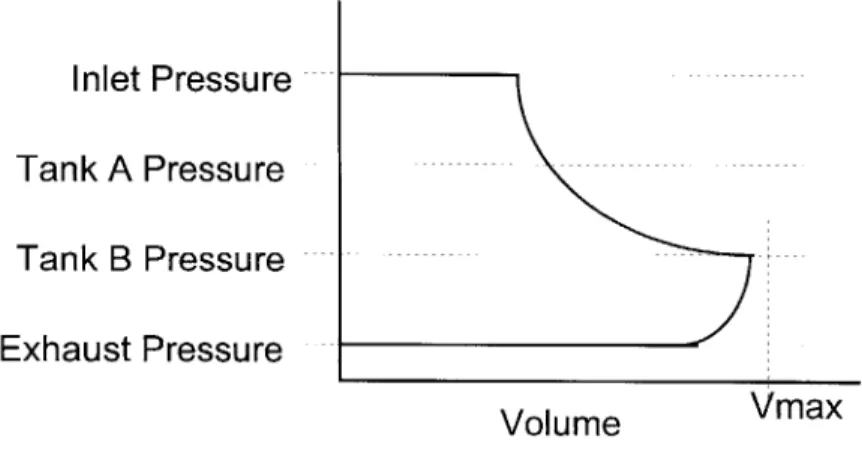
The last scenario considered was a situation in which the relation between V2 and Pb, resulted in a low

stroke for the piston. Figure 8 illustrated the pressure-volume relation for the expander cycle in the cold region.

Inlet Pressure

Tank A Pressure

Tank B Pressure

Exhaust Pressure

Volume

Vmax

Figure 8: Ideal P-V Relation for Low Stroke

In this situation, the pressure in the cold region decreased to PB before the piston reached top dead center. The

isentropic expansion from state 3 to 4 was modeled the same as in the rubber geometry scenario. However, at state

4, there was still a finite volume in the warm region. Therefore, when the exhaust valve was opened, the piston suddenly dropped, expanding the gas remaining in the warm region until the pressure equaled that of the exhaust line. During the process from state 4 to 5, the warm region was modeled isentropicaly, and the cold region was modeled like the rubber geometry model, accounting for the work transfer from the moving piston.

2.3 Optimization

With all the state equations know for the free-piston expander cycle, it was necessary to analyze the system's behavior under various conditions. These equations were first normalized to various system parameters to provide a generalized analysis. The equations were then solved with the Microsoft Excel solver, which allowed target values,

adjustable system parameters, and system constraints to be entered. The resulting steady-state cyclic operating conditions were then tested for stability to determine if non-equilibrium conditions would return to a stable

Before optimizing the state equations, they were normalized to certain system parameters. All temperature variables were normalized to T,, the temperature of the gas entering the cold region of the expander. All pressures were normalized to the inlet line pressure, Pig. The volume variables were normalized to Vmax, the maximum volume of the cylinder occupied by the working fluid. Finally, all the mass variables were normalized to Mref,

defined by the ideal gas relation in equation 17.

in-V max

_ref"

RTin

Eqt 17 The normalized equations for all three models were entered into a spreadsheet for manipulation. Appendix A contains all of the normalized state equations for the free-piston expander.

The objective of the optimization routine was to minimize the value of T*Out~f(V*2, P*A, P*B) by varying the

three independent variables. These independent variables were the volume of the cold region at state 2 and the pressures in the intermediate pressure tanks. These adjustable parameters were subject to the equilibrium constraint that the net mass flow into the intermediate pressure tanks over one cycle must equal zero. The fixed system parameters in the optimization routine were the exhaust line to inlet line pressure ratio and the ambient to inlet line temperature ratio, P*out and T*,.

The rubber geometry model was considered first. For the rubber geometry model, the non-linear

equilibrium constraint was only a function of the pressures in the two intermediate tanks. This fact, coupled with the constraint that the stroke must be matched, allowed the final temperature of the working fluid, T*out, to be optimized as a function of only one variable. Therefore, in addition to the spreadsheet solution, a single algebraic expression for T*out of the rubber geometry model was developed and optimized. The worksheet for this single expression is shown in detail in Appendix B.

In addition, models for systems with three and four intermediate pressure tanks were also developed for the rubber geometry model. These models were used to determine if the improved temperature drop of the working fluid for multiple tanks was significant enough to warrant experimental testing.

The fixed geometry models were considered next. These two models, described earlier, did not provide an optimization routine as a function of only one variable. The value of T*out for the fixed geometry models was

effected by all three independent parameters, and was best optimized by iteration of these parameters in the spreadsheets. There were numerous combinations of the independent variables that satisfied the equilibrium constraint. As expected, only one of the combinations provided optimum cooling for the working fluid.

In addition to the steady state cyclic conditions of the system, the stability of these states were also investigated. To conduct the stability test, non-equilibrium conditions for the system were entered into the

spreadsheet. Using the results of the program, corresponding small iterations in the independent system parameters were made to observe if the system returned to an equilibrium condition or if the system became unstable and failed to recover. Coupled with the stability analysis, were the relative sizes of the intermediate pressure tanks and their effect on the recovery of the system from non-equilibrium cyclic operation. Optimization results are discussed in section 4.1

2.4 Dynamic Modeling

When the free-piston expander was designed, it was critical to understand the piston's behavior during the cycle. Since there was no connection to an external driver, control of the piston was dependent on other system processes and rates. Most of the processes in the expander cycle were assumed quasi-static, except for the blow-in and blow-down process. During these processes there were sudden changes in the pressure differential across the piston, and it was necessary to determine the dynamics of the system to develop an effective control routine.

To model the blow-in process, consider the free body diagram shown below, Figure 9. In this diagram,

FV _FS

Warm End

Piston

Cold End

mpg _FC

Figure 9: Free Body Diagram of Piston

all the forces that acted on the piston during the blow-in process, were represented. FC represented the pressure force in the cold region of the expander.

FC=P in-A c

Eqt 18 In equation 18, Ac represented the cross-sectional area of the piston and Pi,, represented the high-pressure inlet line pressure. The loading of the piston was not modeled as an instantaneous process. Instead, the loading was modeled using an exponential function with a time constant, shown in equation 19.

-t

FC=C-1 - e

Eqt 19 In equation 19, C represented the steady-state loading of the piston.

Recall that in the blow-in process, it was assumed that no mass left the compressed warm region, and as a result, there was a gas spring in the warm region. The resulting force from the gas spring, equation 20, was modeled

as a linear spring with K being the effective spring constant.

FS=K-X

Eqt 20 To obtain a relation for the spring constant, the second law of thermodynamics was employed. Consider the form of the second law where s(V,P), equation 21.

d FS'

-C d A c-X) A c

-C.-

=C.

P

V

Eqt 21 Equation 21 was then rearranged to yield the effective spring constant, K, shown in equation 22. In equation 22, H represented the height of the region occupied by the gas in the warm region.

K=-d(FS) k-P 8-A c

d(X)

H

In Figure 9, the dampening force, FV, was modeled two different ways. First, FV represented the shear stress caused by the thin layer of working fluid between the piston and the cylinder wall, equation 23.

F -A s d(X)

FV=-,

G

d(t)

Eqt 23

In equation 23, G represented the radial distance between the piston and cylinder wall, and As represented the surface area of the piston. Since the shear stress did not provide adequate dampening, FV was then modeled a second way to represent the effect of the orifice. For a fist order analysis, Bernouli's equation for steady state incompressible flow was used to obtain a relation between the warm-end pressure, velocity of the piston and the cross-sectional area to orifice area ratio, Ac/ A₀. Equation 24 shows the result of this model.

1

d(X)

A c

P(t)=P 8 +--p -( - -- -1

2

d(t)

A

Eqt 24

To ensure a linear differential equation, the squared velocity term in equation 24 was approximated with only a first order velocity term by dropping the square.

The resulting governing equations of motion for the two different models are shown below in equation 25 and 26, respectively.

d2 p-As d k-Ac'P 8

Pin-Ac

X +

+

X-X

X=

- g

dt

mP-G dt

mP-H

m

Eqt 25

d 2

_X

_{X+_}

_.-.

_[ii

A

d

k-A c'P 8

P iAe

-

1

-A c-X +

-X=

-g

dt

_{2 mp}

A

dt

mP-H

m

In order to solve these second order ordinary differential equations, algebraic substitutions were made to arrange equation 25 and 26 into the form of equation 27, where C represented the steady-state loading of the piston in equation 26 and 27. -t 2( -d d 2

X +2-P -- X +o )

e

dt

dt

To obtain a solution to the initial-value problem, the Laplace transformation method was employed. Taking the Laplace transform of equation 27, and solving for L[X(t)], yielded the function shown in equation 28.

L (X(t))= C

1 2 2

,u-(s)- s+- -s _{+ 2 -P-s + o 0}

Eqt 28

The next step, involved taking the inverse Laplace transform of equation 28 by use of contour integration. The result of the integration is shown in equations 29 and 30, and Figure 10 illustrated the contour in the s-domain, which was integrated.

~- 01- - fsin(ol-t)+ol - -- cos(o1-t) C -C-e C-e T -I)= +- +I 2 + 2 2

1l

_p01

Poles

_is

I*wl

-BI

-1_ -i*w1

Figure 10: Contour Integration for Inverse Laplace Transform

These models for the dynamics of the piston, were used to investigate the vibration effects during the blow-in process. The results of this analysis were then used to determblow-ine if special consideration was needed blow-in the control routine to monitor the rapid processes. It was equally important to ensure the system did not react

uncontrollably to the sudden change in pressure and damage the testing apparatus. An example of the program used for the dynamic analysis is shown in Appendix F.

3

Design of Free-Piston Expander

3.1 Apparatus Design

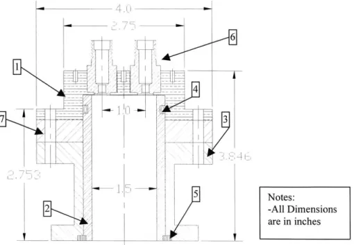
Figure 11 illustrated a detailed sketch of the entire free-piston testing apparatus. The high-pressure Nitrogen line supplied the actuators and the pressure regulated working fluid to the expander. The Nitrogen, used as

the working fluid, was regulated to remove any fluctuations in pressure that were present in the source line. In order to eliminate the flow restriction through the regulator, an inlet surge tank was placed between the regulator and the inlet valve. Since this experiment only consisted of a single stage apparatus, the exhaust line opened directly to the atmosphere.

The warm-end of the cylinder was mounted to a stationary stand through a split-ring and flange. A valve platform and brass cap, containing two throttles, were bolted to the top of the flange. The two throttles were soldered into the brass cap and connected to the 5/2-spool valve, which determined the intermediate pressure tank that was in communication with the warm end of the expander. The pressure tanks, constructed from gas cylinders, were connected to the system through 3/8" copper tubing.

5/2-S ppol Valve

Constant Pressure Throttles (2)

Tanks Brass Cap Valve Platform Warm ---- Flange End ///// /Stationary Support

Cylinder Inlet Surge Tank

Regulator Exhaus

Cold %% -- High Pressure

End Inlet Nitrogen Line

3-Way Multi-Purpose Valves

Actuators

In Figure 11, the cylinder, inlet valve, exhaust valve and inlet surge tank were employed from a previous experiment by Ludwigsen. Design and constuction of the free-piston apparatus focused on the warm-end of the expander and control of the cyclic operation.

3.1.1 Valves

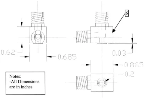
In the free-piston design, the valve sizes and sequencing were critical to control of the expander. the throttle valves, responsible for dissipating the work, were the most critical valve in the design of the apparatus. An angled needle valve, made by Whitey, model B-lRM4-A, was chosen for two reasons. First, using the correlation in equation 31, provided by Minuteman Controls Co., it was determined that a flow factor of Cv=.05 was needed to run test at one Hz, the cyclic frequency for testing.

Cv= 1.024-Q

(P 2 -

Eqt 31 These needle valves had an approximately linear, Cv verses turns opened, relationship in the range of flow

restrictions required for testing. The second factor in choosing these valves involved minimizing the void space when the piston was at top dead center. As shown in Figure 13, the bottom portions of the needle valves were machined flat except for a lip used to index the position of the valves. When the valves were then mounted in the brass cap, as shown in Figure 14, this allowed the valve seats to rest directly above the cylinder, minimizing the void

space between the piston and the orifice. A list of parts for Figure 13 through Figure 15 was located in Table 1 The ROSS 5/2-spool valve, model W7016A233 1, was used for controlling flow between the throttle valves and the intermediate pressure tanks. This valve allowed for two configurations of testing, illustrated in Figure 12. Configuration (I) used one of the throttle valves, and sealed ports one and three. Toggling the solenoid on and off selected the intermediate pressure tank, which was connected to the warm end through throttle 1. Configuration (II) employed two throttles, and only port four was sealed. Testing in this configuration allowed the throttling into each of the pressure tanks to be controlled independently. As configuration (II) illustrated in Figure 12, throttle 1 controlled the gas flow into tank A and throttle 2 controlled the gas flow into tank B. Although configuration (II) had no effect on the thermodynamic model, it provided variable control of the dynamics of the cycle.

Warm Region > Warm Region >

T9

Thr

Miel

C

1 2 1 2

(B) (A)

(B) (A

Intermediate Pressure Tanks

Configuration (I

)

0

(B)

(A)

Intermediate

Configuration ( I

(B)

(A)

Pressure Tanks

I )

Figure 12: Spool Valve Configurations

List of Parts(figures 13-15)

Part # Name Notes

1 Brass Cap Brass

2 Cylinder Stainless Steel 3 Flange Stainless Steel

4 O-Ring Rubber

5 Split-Ring Stainless Steel

6 Throttle Brass

7 Valve Platform Carbon Steel Table 1: List of Parts for Figures 13-15

6

Notes:

-All Dimensions are in inches

Figure 13: Machined Throttle Valves

3.1.2 Flange

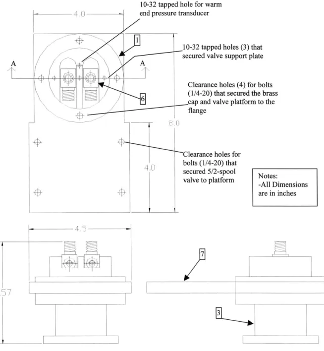
As shown in Figure 11, the testing apparatus was suspended from a stationary support. To mount the apparatus, the flange, which bolted to a testing stand, held a split ring in place around the cylinder, Figure 15. With the flange attached to the testing stand, it became the stationary point to which the valve platform and brass cap were bolted. The clearance holes for the bolts can be seen in both Figure 14 and Figure 15.

3.1.3 Brass Cap

One of the most critical components in the warm end assembly was the brass cap. The cap had to be machined in such a manner as to minimize the void space in the cylinder at top dead center and provide a static seal for the warm end of the expander. Figure 15 showed the relative position of the two throttles to the top of the cylinder. The throttles were soft soldered to the brass cap and a support plate was screwed down on top of the valves to provide extra stability. As illustrated, the seats on the throttles rested just above the top dead center position of the cylinder. This minimized the void space above the piston at state 4 of the cycle.

The brass cap also provided a static seal for the warm end of the expander. As illustrated in Figure 15, the outside of the cylinder was turned to allow for a 1/8", male gland, o-ring. This o-ring provided a static seal to the inside bore of the brass cap when the cap was securely bolted to the flange.

10-32 tapped hole for warm end pressure transducer

10-32 tapped holes (3) that secured valve support plate A

Clearance holes (4) for bolts (1/4-20) that secured the brass cap and valve platform to the flange

Clearance holes for bolts (1/4-20) that secured 5/2-spool

valve to platform Notes:

-All Dimensions are in inches

4,2

7

3

Figure 14: Warm-End Assembly

5 _Notes:

-All Dimensions are in inches

Figure 15: Assembly Cross-Section View A-A

3.1.4 Piston

The piston was constructed from a G- 10, thin-walled, cylinder filled with foam, and the ends of the piston were attached using STYCast 1266 epoxy encapsulate. There were three main considerations for the piston design. First, the length of the piston was chosen to be 35.485" in length, which resulted in a 1.528" stroke. The piston was then turned down to a final diameter of 1.492", which determined the clearance between the piston and cylinder wall to be .008". The clearance needed to be small enough to restrict the flow around the outside of the piston during the expansion process, but not too small that the errors in both the cylinder and piston would result in drag between the cylinder wall and piston.

The final consideration for the piston is illustrated in Figure 16. Although there were no physical connections to the piston, its exact position and velocity were critical to the control routine.

recess for ferro-magnetic shim

Figure 16: Warm End Sketch of Piston

To determine the position of the piston, a linear variable differential transformer (LVDT) was designed and integrated into the piston and cylinder. A ferro-magnetic steel shim (.002" thick) was epoxied into the machined recess on the piston wall, illustrated in Figure 16. The operation of the LVDT will be discussed in section 3.2.1.

3.2 Instrumentation and Signal Conditioning

Instrumentation for the free-piston apparatus was required for two reasons. First, data needed to be collected and compared with the optimized models to analyze the performance of the expander. More importantly, it was necessary to monitor the status of the expander to provide information to the control routine. It was essential that the pressure in the expander and position of the piston were monitored adequately to provide information about the transient behavior of the system. Although the thermal performance of the system was not a focus of the experiment, temperature measurements for the inlet and exhaust lines were also obtained.

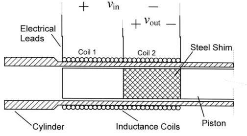
3.2.1 Linear Variable Differential Transformer

To detect the position of the piston, a LVDT was designed and integrated into the cylinder and piston. Figure 17 provided a cross-sectional view of the LVDT as it was mounted on the apparatus. The Inductance coils were wound around the warm-end of the thin-walled cylinder. The windings formed two double-layer coils with a center tap between the two coils. An AC excitation voltage, shown as vij in Figure 17, was applied across the full length of the two coils, and the output voltage, vent, determined the position of the piston inside the expander. Equation 32 illustrates that the output voltage from the LVDT was in phase with the excitation voltage and the magnitude was controlled by the relative inductance of the two coils.

v gn -L2

v out= -. cos(cO -)

L1 +L2

Eqt 32

Vi and co were the amplitude and frequency of the excitation voltage, respectively. LI and L2 were the respective

inductance values for the two coils.

The inductance of the two coils was varied by the location of the steal shim epoxied to the piston.

+

Electrical

+

Vout

-Leads

Leads

_\Steel

Shim,

Cylinder

Inductance Coils

Piston

Figure 17: Cross-Sectional View of LVDT

The inductance of each individual coil was increased as the shim entered the core of that coil. The steal shim was mounted on the piston, relative to the pick-up coils, such that the output signal from the LVDT was in the linear range for the given stroke length. Calibration curves for all of the instrumentation can be found in Appendix C.

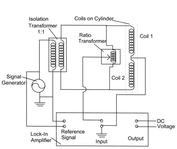
The output signal from the LVDT was conditioned using the circuit illustrated in Figure 18. The bridge consisted of the two coils wound on the outside of the cylinder. The coils were in parallel with an adjustable ratio transformer. The parallel coils and transformer formed the two legs of an inductance bridge. The ratio transformer allowed precision adjustments in the inductance ratios to balance the bridge. Even with the bridge balanced, the AC output signal was not compatible with data acquisition system. It was necessary to convert the 6 KHz AC signal to a DC signal that would vary with the position of the piston. To achieve this conversion, a lock-in amplifier was employed. The amplifier in Figure 18 multiplied the reference signal and input signal together to yield equation 33.

Vref _{and vinput were the respective amplitudes and x represented the phase shift of the input signal with respect to the}

v input v ref

2

-(cos(2o -t + a) + cos(a))

Eqt 33 Passing this result through a low-pass filter, the amplifier then output the signal represented by equation 34.

V input-V ref

2

(cos(a))

Isolation

Transformer

1:1 \

Coils on Cylinder

DC

Voltage

Figure 18: LVDT Electrical Schematic

Consider a balanced bridge in Figure 18 with the shim center between the two coils, if the ferro-magnetic core entered coil 2, the input signal to the amplifier became negative and was 180 degrees out of phase with the reference signal. As the steel core moved back to the center of the two coils, the magnitude of the negative DC output signal decreased to zero. The two signals were then in phase as the core passed into coil 1, producing a

positive DC signal proportional to the position of the piston. The 1:1 isolation transformer was used to eliminate a ground loop since both the signal generator and an input signal terminal were grounded.

3.2.2 Pressure

Both static and dynamic pressure conditions were monitored throughout the apparatus. Static pressure measurements were obtained manually from gauges on the regulated inlet line and the intermediate pressure tanks. These locations in the system were maintained at constant pressure and were not needed for the control routine. However, the transient behavior of the pressure inside the expander was required in the control routine.

In the warm region, an ENDEVCO strain gauge pressure transducer, model AG497, was threaded into a pressure tap machined in the brass cap. The signal from this transducer was routed through an ENDEVCO, model 4428A, pressure indicator which had a five volt F.S.O. The transient pressure in the cold region of the expander was monitored by a KISTLER, model 603B3, piezo-quartz pressure transducer. The signal was then processed in a KISTLER, model 5004, charge amplifier with a ±10 volt F.S.O.

3.2.3 Temperature

Although the focus of the experiment was not the actual cooling of the working fluid, temperature measurements for both the inlet and exhaust lines were acquired by the data acquisition system. Type E, chromel and constantan, thermocouples were used along with their appropriate cold-junction compensator units. The inlet thermocouple was soldered into a tube fitting, which was mounted on the lower end of the inlet surge tank. The exhaust line thermocouple was placed in the flow of the exhaust gases. Since the exhaust line was opened to the atmosphere, transient behavior in the temperature was observed between the surge of exhaust gas and the exhaust line being back-filled with atmospheric gases. An average over several cycles was used to eliminate these fluctuations in data.

3.3 Control Design

The free-piston expander was monitored with a DAS-20 data acquisition board, manufactured by Keithley MetraByte Corporation. The DAS-20 monitored the two pressure transducers, two thermocouples and the LVDT. The digital output from the DAS-20 controlled the inlet and exhaust valves along with the 5/2-spool valve on the warm end of the expander.

The control program, written in QBasic 4.5, utilized pre-defined, machine language, call routines to perform all I/O operations. All required calculations to control the system were performed within the QBasic program. The program, shown in Appendix D, was divided into a manual mode and an automatic mode, which provided complete control of the expander and data storage.

The manual mode served two purposes. First, the manual mode was used to initialize the system for cyclic operation and troubleshoot any problems in the system. Second, this mode was used to transfer data from Basic arrays, acquired during automatic operation, to disk for manipulation. The six permissible operations in this mode are shown in Table 2.

KEY PRESS

OPERATION

I Toggle inlet valve opened/closed E Toggle exhaust valve opened/closed

T Toggle 5/2-Spool Valve

A Write QBasic data array to A:\ drive

B Begin automatic operation

X Terminate program and return to code

Table 2: Options in Manual Mode

Figure 19: Flowchart for Automatic Mode