HETEROFOR 1.0: a spatially explicit model for exploring the response of structurally complex forests to uncertain future conditions. II. Phenology and water cycle

HAL Id: hal-02466109

https://hal.umontpellier.fr/hal-02466109

Submitted on 4 Feb 2020

HAL is a multi-disciplinary open access

archive for the deposit and dissemination of

sci-entific research documents, whether they are

pub-lished or not. The documents may come from

teaching and research institutions in France or

abroad, or from public or private research centers.

L’archive ouverte pluridisciplinaire HAL, est

destinée au dépôt et à la diffusion de documents

scientifiques de niveau recherche, publiés ou non,

émanant des établissements d’enseignement et de

recherche français ou étrangers, des laboratoires

publics ou privés.

cycle

Louis de Wergifosse, Frédéric André, Nicolas Beudez, François de Coligny,

Hugues Goosse, François Jonard, Quentin Ponette, Hugues Titeux, Caroline

Vincke, Mathieu Jonard

To cite this version:

Louis de Wergifosse, Frédéric André, Nicolas Beudez, François de Coligny, Hugues Goosse, et al..

HETEROFOR 1.0: a spatially explicit model for exploring the response of structurally complex forests

to uncertain future conditions. II. Phenology and water cycle. Geoscientific Model Development,

European Geosciences Union, 2020, 13, pp.1459-1498. �10.5194/gmd-2019-201�. �hal-02466109�

1

HETEROFOR 1.0: a spatially explicit model for exploring the

response of structurally complex forests to uncertain future

conditions. II. Phenology and water cycle.

Louis de Wergifosse

_{, Frédéric André}

_{, Nicolas Beudez}

_{, François de Coligny}

_{, Hugues Goosse}

_,

François Jonard

, Quentin Ponette

, Hugues Titeux

, Caroline Vincke

, Mathieu Jonard

5

1_{Earth and Life Institute, Université catholique de Louvain, Louvain-la-Neuve, 1348, Belgium}

2_{Botany and Modelling of Plant Architecture and Vegetation (AMAP) Laboratory, Institut National de la Recherche}

Agronomique (INRA), Montpellier, 34398, France

Correspondence to: Louis de Wergifosse (louis.dewergifosse@uclouvain.be)

Abstract

Climate change affects forest growth in numerous and sometimes opposite ways and the resulting trend is often difficult to predict for a given site. Integrating and structuring the knowledge gained from the monitoring and experimental studies into process-based models is an interesting approach to predict the response of forest ecosystems to climate change. While the first 5

generation of such models operates at stand level, we need now individual-based and spatially-explicit approaches in order to account for structurally complex stands whose importance is increasingly recognized in the changing environment context. Among the climate-sensitive drivers of forest growth, phenology and water availability are often cited as crucial elements. They influence, for example, the length of the vegetation period during which photosynthesis takes place and the stomata opening, which determines the photosynthesis rate.

10

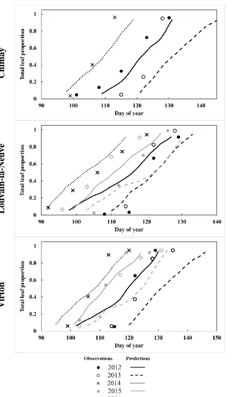
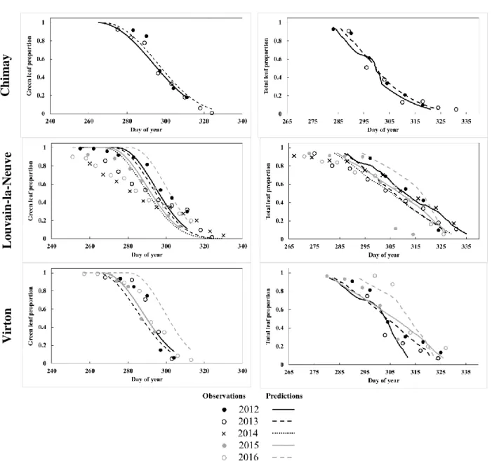
In this paper, we describe the phenology and water balance modules integrated in the tree growth model HETEROFOR and evaluate them on six Belgian sites. More precisely, we assess the ability of the model to reproduce key phenological processes (budburst, leaf development, yellowing and fall) as well as water fluxes.

Three variants are used to predict budburst (Uniforc, Unichill and Sequential), which differ regarding the inclusion of chilling and/or forcing periods and the calculation of the coldness or heat accumulation. Among the three, the Sequential approach is 15

the least biased (overestimation of 2.46 days) while Uniforc (chilling not considered) best accounts for the interannual variability (Pearson’s R = 0.68). For the leaf development, yellowing and fall, predictions and observation are in accordance. Regarding the water balance module, the predicted throughfall is also in close agreement with the measurements (Pearson’s R = 0.856, bias = -1.3%) and the soil water dynamics across the year is well-reproduced for all the study sites (Pearson’s R comprised between 0.893 and 0.950, and bias between -1.81 and -9.33%). The positive results from the model 20

assessment will allow us to use it reliably in projection studies to evaluate the impact of climate change on tree growth and test how diverse forestry practices can adapt forests to these changes.

3

1 Introduction

Forests play an important role in regulating the climate system as their evapotranspiration and land surface properties (e.g. albedo, roughness) determine water and energy exchanges with the atmosphere (Stocker et al., 2013; Naudts et al., 2016). Moreover, given the forest ability to sequester carbon in biomass and soil, they also affect climate by acting on the global carbon cycle (Schlamadinger and Marland 1996; Whitehead, 2011; Le Quéré et al., 2017). Forest ecosystems also provide 5

many other services such as biodiversity conservation, soil and water protection and recreation (Millennium Ecosystem Assessment, 2005). The extent to which the provision of these services will be ensured in the future is however quite uncertain and depends on the response and adaptability of these ecosystems to global changes (Lindner et al., 2010).

Forests experience numerous and fast perturbations in the context of anthropogenic global changes: physical environment modifications such as increasing CO2 (Reyer et al., 2014) and O3 concentrations (Lorenz et al., 2010; Ainsworth et al., 2012),

10

rising nitrogen depositions (Solberg et al., 2009) or climate change (Boisvenue and Running, 2006) coupled to landscape fragmentation and the subsequent biodiversity loss (Fahrig, 2003), the appearance of pests (Williams and Liebhold, 1995; Flower et al., 2015), diseases (Desprez-Loustau et al., 2006; Sturrock et al., 2011) and invasive species (Walther et al., 2009) as well as the modification of forest management practices (Noormets et al., 2015) linked to the evolution of forestry paradigms and society (Raum and Potter, 2015). In this study, we focus on climate change. According to European climate projections of 15

the last IPCC report (Kovats et al., 2014), all Europe will face a temperature increase between 1 and 5.5°C depending on the greenhouse gas emission scenario (Jacob et al., 2014). The temperature rise will be especially important in summer in the South of Europe and in winter in Northern Europe, leading among others to a decrease in the frequency of frost day occurrence. Rainfall projections vary more regionally. A precipitation trend gradient should appear with 25% wetter climate conditions in the North and 15% dryer ones in the South while no clear trend emanates for continental Europe (Jacob et al., 2014). Moreover, 20

in most of Europe, rainfall is expected to increase in winter and decrease in summer. Finally, climate extremes are projected to increase for the whole continent. In particular, the frequency of heat waves, the length of droughts and the magnitude of heavy rainfall events are likely to rise while a short increase in wind speed extremes could occur in winter over the Centre and the North of Europe.

The rapidly changing climate has already affected the forest productivity, which has globally increased since the middle of the 25

20th century (Boisvenue and Running, 2006). In North-Eastern France and Belgium, for example, beech productivity increased on average by 50% during the 20th century (Aertsen et al., 2014, Bontemps et al., 2010, 2011, 2012, Charru et al., 2010). Overall, the two main processes regulating forest growth, photosynthesis and respiration, are both stimulated by climate changes. While the higher temperatures in spring trigger earlier budburst and therefore extend the photosynthesis period (Menzel et al., 2006; Park et al., 2016), the rise in atmospheric CO2 increases the photosynthesis rate due to higher intercellular

30

CO2 concentrations (Ainsworth and Long., 2005; Thompson et al., 2017). For Europe, Menzel et al. (2006) detected an advance

in the budburst, flowering and fruiting dates at a rate of 2.5 days per decade between 1971 and 2000. Regarding CO2-fertilizing

when ambient carbon dioxide concentrations were elevated to 550 ppm (Norby et al., 2005; Norby et al., 2010). In parallel, photosynthesis and maintenance respiration are favoured by the increase in air temperature (Aber et al., 2001; Yamori et al., 2014). Yet, there is no consensus on which of respiration and photosynthesis sensitivity to temperature will have the dominant effect (Zhang et al., 2017). Overall, so far, even if the enhanced photosynthesis has been attenuated by a higher maintenance respiration, the resulting climate change impact has been an increased forest productivity when soil water and nutrient 5

availability were not limiting (Boisvenue and Running, 2006). For the sites with a low extractable water reserve, the water stress experienced by the trees could intensify in the future due to increasing evapotranspiration rates and more frequent summer droughts. With the soil drying, photosynthesis is progressively reduced due to stomatal closure and the net primary production (NPP) is decreased. If the soil water potential approaches the wilting point such as in 1976, 2003 and 2018 in Europe, vitality loss and even tree mortality may occur due to carbon starvation and/or hydraulic failure depending on the tree 10

species strategy to cope with water stress (Ciais et al., 2005; McDowell, 2011; Choat et al., 2012). However, higher CO2 levels

increases the water use efficiency (Keenan et al., 2013) and allow the trees to reduce their stomatal conductance while maintaining the photosynthesis active (Leuzinger and Körner, 2007; Franck et al., 2015).Besides this water stress, the response of forest ecosystems to increased atmospheric CO2 is constrained by nutrient availability including nitrogen, to the point of

not responding at all on the nutritionally poorest sites (Oren et al., 2001; Fernandez-Martinez et al., 2014). 15

Since climate change affects some processes positively and others negatively and given the interactions among factors as well as the feedback and acclimation mechanisms, it is not easy to predict the resulting effect of climate change on tree growth at a given site (Lindner et al., 2014; Herr et al., 2016). Knowledge about climate change has been acquired based on long-term monitoring studies that are limited to the observed changes and on experiments of environment manipulation generally analysing one or two factors at a time on a limited period (CO2 enrichment, rainfall exclusion…). In order to apprehend the

20

complex functioning of forest ecosystems, the use of process-based modelling is a complementary approach that allows to integrate and structure the existing knowledge and to make extrapolations for unprecedented conditions like those projected for the coming decades.

Process-based models were originally built to predict forest growth response to environmental changes at stand level without accounting for management operations and canopy heterogeneity. Such models were therefore suitable for pure even-aged 25

stands but hardly manage to simulate mixed and structurally-complex stands (Pretzsch et al., 2007). Yet, nowadays, a promising way to adapt forests to climate change is to progressively turn them into uneven-aged and mixed stands using continuous cover forestry and natural-disturbance based management to improve their stress resistance and resilience (Messier et al., 2015). To account for the spatial heterogeneity, some process-based models were designed or adapted to simulate various tree cohorts (characterized by a same species and size class). Yet, this approach only considers the vertical dimension of spatial 30

heterogeneity while implementing innovative forestry practices in structurally-complex stands requires to account for the horizontal dimension through a spatially-explicit approach at tree level (Pretzsch et al., 2007; Fontes et al., 2010).

5

Several papers have demonstrated that this level of spatial description is crucial for addressing hydrological questions. For, example, individual evapotranspiration strongly depends on the radiation intercepted by the tree and on the local resistance to water vapour transfer. For the same open-air climate conditions, two trees with identical dimensions can have different evapotranspiration rates if they experience contrasted light and wind conditions due to the size, density and species composition of their neighbours. Not accounting for this local conditions using one or two dimensions approaches can generate errors in 5

the evapotranspiration calculation at the tree and stand levels (Flerchinger et al., 2015; Vezy et al., 2018).

As the models of this particular type are very few (Simioni et al., 2016) and generally do not take into consideration tree nutrition and nutrient cycling (or in a very simplified way), we decided to develop a new model called HETEROFOR (for HETEROgeneous FORests). This model describes tree growth dynamics based on mechanistic approach in structurally-complex stands and in a changing environment. It is based on resource sharing and integrates the main abiotic productivity 10

and vitality factors. The creation of a new model was driven as well by the fact that the comparison of models of the same type are interesting to evaluate conceptual differences and uncertainties, to highlight the relative importance of processes and to determine their optimal level of description according to the question addressed.

The processes regulating the carbon fluxes and the dimensional growth constitute the core of the HETEROFOR model and are described in Jonard et al. (in review, 2019). Here, we focus on the description of two modules essential for predicting the 15

impact of climate change on tree growth: phenology and water balance. In addition, we used data from long-term forest monitoring to evaluate the capacity of the model to reproduce key phenological phases (budburst, leaf development, yellowing and fall) and the soil water content dynamics as well as to estimate throughfall and deep drainage. Evaluating each module separately is necessary to ensure the consistency of the whole model and to avoid that different error types compensate each other. Given the number of parameters, good predictions can often be obtained on integrative variables such as the diameter at 20

breast height (dbh) increment but this is not sufficient to guarantee the quality of the model. A realistic evaluation should test each module component separately with independent data and then assess the overall model quality of predictions (Soares et al., 1995).

2 Material and Methods

2.1 Model description

2.1.1 Overall model

HETEROFOR is a model hosted in CAPSIS (Computer-Aided Projections of Strategies In Silviculture), a software platform for forest growth simulations (Dufour-Kowalski et al., 2012) that provides the execution system and procedures to run 5

simulations and display the outputs. Still, apart from these data structures and operative methods, all initialisation and evolution procedures are specific to HETEROFOR. The initialisation phase of the model consists in loading different files (tree species parameters, tree and stand characteristics, chemical and physical soil properties, meteorological data and fruit production data) in order to create trees and soil horizons. Then, tree growth is calculated yearly according to the HETEROFOR methods presented in Jonard et al. (in review, 2019). So far, HETEROFOR is adapted and calibrated only for deciduous species but the 10

adaptation to evergreen species is under progress.

Once the initialisation is completed, the first routine called is the calculation of phenological periods from meteorological data, which is described is Sect. 2.1.2. This function provides key phenological dates and daily foliage state (proportions of leaf biomass and of green leaves relatively to full leaf development) for each day during the year. These phenological outputs are notably used for the radiation balance carried out using the SAMSARALIGHT library coupled to HETEROFOR (Courbaud 15

et al., 2003). According to a ray tracing approach and based on the solar radiation measurements from the meteorological file, this library differentiates the direct and the diffuse components from the global radiation and determines for both components the part of energy absorbed by the crown and the trunk of each tree and the part that reaches forest floor. All this information is required to estimate evapotranspiration components and tree photosynthesis. All aboveground and belowground water fluxes are calculated according to the processes described in Sect. 2.1.3, which allows to perform a water balance for each soil horizon 20

and to update its soil water content.

GPP is estimated for each individual tree using the photosynthesis method implemented in the model CASTANEA of CAPSIS (Dufrêne et al., 2005). The sunlit and shaded leaf proportions, the direct and diffuse photosynthetically active radiation (PAR) absorbed per unit of leaf area and the mean soil water potential are required as input variables for CASTANEA. A part of the GPP is used for growth and maintenance respiration, the remaining part constituting the NPP. Maintenance respiration can be 25

estimated as a fraction of the GPP or calculated for each tree compartment by a method accounting for the living biomass, its nitrogen concentration and a Q10 function that describes the temperature dependence. Growth respiration corresponds to a

fraction of the carbon used to build the new tissues. NPP is then distributed to the different tree compartments (branches, trunk, roots, leaves) giving priority to the functional organs, namely, leaves and fine roots. The carbon sharing between these two sinks depends on the tree nutritional status, trees with a poorer nutrient status allocating relatively more carbon to fine roots. 30

7

allometry relationships. All these processes involving carbon fluxes are described in details in Jonard et al. (in review ,2019). The HETEROFOR model also contains a tree nutrition and nutrient cycling module that will be described in a future paper.

2.1.2 Phenological module

The phenological module aims at simulating the evolution of leaf from budburst to yellowing and leaf fallin order to update the foliage status at a daily time step, namely, the proportions of leaf biomass and of green leaves relatively to complete leaf 5

development. These two foliage properties are key variables to simulate energy, water and carbon fluxes within the forest ecosystem. The leaf biomass proportion calculated for each tree species allows to predict the seasonal evolution of the individual leaf area. The first leaf appearance triggers the start of the leaved period running until all the leaves have fallen. The proportion of green leaves impacts photosynthesis and tree transpiration, as these processes are not active anymore on discoloured leaves. When leaves start yellowing, they still intercept rainfall while their photosynthetic activity and their 10

transpiration are progressively reduced.

The following phenological phases are distinguished, in chronological order:

- Chilling period: accumulation of coldness that breaks the dormancy. It is initiated at the chilling starting date (t0) and

ends at the forcing starting date (t1).

- Forcing period: accumulation of heat that initiates the leaf development in the bud and leads to the budburst (budburst 15

date = t2a).

- Leaf development: progressive growth of the leaves from budburst to the complete leaf development (leaf development date = t2b).

- Ageing: accumulation of coldness that is initiated at the ageing starting date (t3) and ends at the yellowing starting

date (t4a).

20

- Yellowing: loss of photosynthetic activity linked to the decrease of day length. This phase ends at the yellowing ending date (t4b).

- Falling: the fall of the dead leaves starts (t5a) when less than 60% of the leaves are still green and continues until the

leaf fall ending date (t5b).

Since the phenological timing can vary considerably between species, the phenology dates are calculated for each tree species 25

separately. Intra-specific differences are also likely to occur according to the age or social status (Cole and Sheldon, 2017) though are not considered here.

The phenological module is optional in HETEROFOR. Activating the phenology requires an hourly meteorological file. If not activated, the model uses identical budburst and leaf fall dates for all years and tree species set by the user.

The principle behind the whole phenology module is similar for each phase. A state variable is increasing progressively 30

growing at a rate depending on meteorological conditions (mainly air temperature). When the phase state reaches a certain

Three common models are implemented so far to calculate the average budburst date (t2a): the Uniforc (Chuine, 2000), the

Unichill (Chuine, 2000) and Sequential (Kramer, 1994) models. The first only considers forcing while the latter ones integrate both chilling and forcing.

The Unichill model starts to operate when the day of year corresponds to the chilling starting date (t0). At this moment, the

daily chilling rate (Rc) is calculated according to

5 𝑅𝑐= { 1 1+𝑒𝐶𝑎(𝑇−𝐶𝑐)2+𝐶𝑏(𝑇−𝐶𝑐), −5 ≤ 𝑇 ≤ 10 0, 𝑇 > 10 𝑜𝑟 𝑇 < −5 (1) with

Ca, Cb and Cc (°C), chilling parameters T, the daily average temperature (°C).

This rate is summed each day until reaching the chilling threshold (C*) that triggers the forcing starting date (t1). For the

10

Uniforc model, t1 is fixed. Regarding the forcing period, the forcing rate (Rf) is calculated using the following equation in both

models : 𝑅𝑓= { 1 1+𝑒𝐹𝑏(𝑇−𝐹𝑐), 𝑇 > 0 0, 𝑇 ≤ 0 (2) with Fb and Fc (°C), parameters. 15

The budburst is activated when the sum of the daily forcing rates equals the forcing threshold (F*). For the sequential model, the following equations are considered for Rc and Rf :

𝑅𝑐= { 0, 𝑇 ≤ 𝑇𝑚𝑖𝑛 𝑇−𝑇_𝑚𝑖𝑛 𝑇_𝑜𝑝𝑡−𝑇_𝑚𝑖𝑛, 𝑇𝑚𝑖𝑛 < 𝑇 ≤ 𝑇𝑜𝑝𝑡 𝑇−𝑇𝑚𝑎𝑥 𝑇𝑜𝑝𝑡−𝑇𝑚𝑎𝑥, 𝑇𝑜𝑝𝑡 < 𝑇 ≤ 𝑇𝑚𝑎𝑥 0, 𝑇 ≥ 𝑇𝑚𝑎𝑥 (3) 𝑅𝑓= 𝑎 1+𝑒−𝑏(𝑇−𝑐) (4) with 20

Tmin, Tmax and Topt, the minimum, maximum and optimal temperatures (°C), respectively,

a , b and c (°C), forcing parameters.

The reason for this multi model implementation is that phenological model efficiency is extremely site-dependent (White et al., 1997). For example, studies have often shown that the models including chilling were less precise in Northern locations with generally sufficient cold accumulation to break dormancy (Leinonen and Kramer, 2002). Therefore, the choice of the 25

model should be done by the user with regards to the site.

As the data used for the calibration represented the phenology of an average tree, the model shifts forward the start of the budburst by half the mean budburst period (extending from the budburst date of the earliest tree to that of the latest) in order

9

to consider the start of the budburst of the earliest trees. The length of the budburst period was determined from the different sites used for the evaluation where the phenological observations were conducted on 20 trees.

Once the budburst starting date (t2a) is calculated, the equations for the subsequent phenological variables are the same. The

leaf development rate (Rld) is cumulated daily until the leaf development threshold (LD*) is reached. It is computed according

to: 5

𝑅𝑙𝑑= {𝑇, 𝑇 > 0 _{0, 𝑇 ≤ 0} (5)

where T is the daily average temperature of the current day (°C). The leaf proportion (leafProp, g g-1_{) is calculated for each day according to}

𝑙𝑒𝑎𝑓𝑃𝑟𝑜𝑝𝑡= ∑𝑡_𝑡2𝑎𝑅𝑙𝑑

𝐿𝐷∗ (6)

with 10

t, the current day.

A constant date, defined according to Dufrêne et al. (2005), is considered for the start of the ageing process (𝑡3). This process does not alter leaf quality but is a prerequisite for leaf yellowing (t4a) that is initiated when the cumulated daily ageing rate

(Rage) equals the ageing threshold (A*), with

𝑅𝑎𝑔𝑒= {

𝑇𝑏_𝑎𝑔𝑒− 𝑇, 𝑇 < 𝑇𝑏_𝑎𝑔𝑒

0, 𝑇 ≥ 𝑇𝑏_𝑎𝑔𝑒 (7)

15

with

𝑇𝑏_𝑎𝑔𝑒, the base temperature for ageing (°C).

The leaf yellowing calculation gives the green leaf proportion, greenProp (g g-1_{), which provides the fraction of remaining}

green leaves compared to the maximum green leaf amount. It is set to 1 before the start of yellowing, and then decreases with day length according to the following equation:

20 𝑔𝑟𝑒𝑒𝑛𝑃𝑟𝑜𝑝𝑡= 𝑔𝑟𝑒𝑒𝑛𝑃𝑟𝑜𝑝𝑡−1∗ ( 𝐷𝐿𝑡−𝐷𝐿𝑚𝑖𝑛 𝐷𝐿𝑡4𝑎−𝐷𝐿𝑚𝑖𝑛) 𝑦 (8) with

DLt and DLt4a, the day lengths (hours) for the current day and t4a, respectively,

DLmin, the minimum day length (hours) value over the year, and

Y, a parameter.

25

The day length (hours) is calculated according to Teh (2006):

𝐷𝐿 =24

𝜋 ∗ 𝑎𝑐𝑜𝑠 (−

sin(𝛿)∗sin (𝜆)

cos(𝛿)∗cos (𝜆)) (9)

where λ is the site latitude (rad) and δ, the solar declination (rad) determined as 𝛿 = −23.45∗𝜋

180 ∗ 𝑐𝑜𝑠 (2𝜋 𝐷𝑂𝑌+10

365 ) and DOY is the day of year (i.e., Jan 1=1, Jan 2=2, Feb 1=32…).

The yellowing phase ends when the green leaf proportion reaches 0. The leaf fall (𝑡5) is set to start rapidly after yellowing initiation, namely, when greenProp reaches 0.60, considering that leaves no longer photosynthetically active can quickly fall. The leaf fall rate (Rfall) is calculated daily and is used to update leafProp. It depends on the wind and frost episodes. While the

frost weakens the leaf petiole, the wind can break it and take away the leaf. For this reason, leafProp is determined as follows for each day t:

5

𝑙𝑒𝑎𝑓𝑃𝑟𝑜𝑝𝑡= 𝑙𝑒𝑎𝑓𝑃𝑟𝑜𝑝𝑡−1− 𝑓𝑎𝑚𝑝𝑙∗ 𝑊𝑆 ∗ 𝑅𝑓𝑎𝑙𝑙 (10)

with

fampl, a frost amplifier coefficient fixed to 1 before the occurrence of five consecutive hours with air temperature below

0°C and is then set to 2 and 3 for oak and beech, respectively,

WS is the daily average wind speed (m s-1_),

10

Rfall is the falling rate (s m-1 d-1) calibrated as described in Sect. 2.2.

According to Eq. (10), leafPropt progressively decreases from 1 to 0 while it cannot take a value below greenPropt, accounting

for the fact that green leaves are not expected to fall. Finally, when all leaves have fallen, the trees enter in the leafless period until the budburst of the following year.

2.1.3 Water balance module

15

The water balance module operates at an hourly time step and simulates the sharing of incident rainfall into the main forest water fluxes and pools, namely, interception (i.e., water storage on foliage and bark, and evaporation), throughfall, stemflow, water movements between soil horizons and deep drainage, transpiration and soil water uptake in the different soil horizons, and soil evaporation (Fig. 1). Surface runoff and groundwater level rise are not yet included at this stage.

In a first step, the parameters considered as constant during the leaved and leafless periods are estimated: maximum foliage 20

and bark storage capacities, throughfall and stemflow proportions (described hereafter) and absorbed radiation proportions. Then, the various water fluxes are calculated at an hourly time step.

Foliage and bark storage capacity

The maximum foliage storage capacity of the stand (Cfoliage_max, l) is calculated by summing the storage capacity of each tree

25

species:

𝐶𝑓𝑜𝑙𝑖𝑎𝑔𝑒_𝑚𝑎𝑥 = ∑ (A𝑠𝑝 𝑙𝑒𝑎𝑓_𝑠𝑝 . 𝑐𝑓𝑜𝑙𝑖𝑎𝑔𝑒_𝑠𝑝) (11)

with

A𝑙𝑒𝑎𝑓_𝑠𝑝, the leaf area of all the trees of species sp (m²),

cfoliage_sp, the foliage storage capacity for that species (mm or l per m² of leaf).

11

Bark storage capacity depends on the season (i.e., leafed and leafless periods) and on the tree species. It is derived from a linear model proposed by André et al. (2008a) predicting the individual stemflow (sf, l) produced during a rain event as a function of tree girth (C130, cm) and rainfall amount (R, mm):

𝑠𝑓 = 𝑎 + 𝑏 . 𝐶130 + 𝑐 . 𝑅 + 𝑑 . 𝐶130 . 𝑅 + 𝜏 + 𝛿 + 𝜀 (12)

where a (l), b (l cm-1_{), c (m²) and d (m² cm}-1_{) are fixed effect parameters varying with the species and the season and}

5

𝜏 and 𝛿 are random factors characterizing the tree and the rain event variability.

As it multiplies the rainfall amount in Eq. (12), the term “c + d.C130” may be interpreted as an estimation for the stemflow rate (sfrate, l mm-1). In other respects, André et al. (2008a) determined rainfall thresholds for stemflow appearance (Rmin, mm),

defined as the amount of rainfall required to produce stemflow at the base of the trunk. This threshold was found to be independent of tree size while it depends on both the season and the species. Multiplying the sfrate estimations by Rmin values

10

for the corresponding species and season provides estimates of the tree bark storage capacity (cbark, l), namely, the amount of

water accumulated on branch and trunk bark before stemflow occurs at tree base:

𝑐𝑏𝑎𝑟𝑘= (𝑐 + 𝑑 ∙ 𝐶130) ∙ 𝑅𝑚𝑖𝑛 (13)

The individual cbark estimates are then summed over all trees for each season to determine leafless and leaved stand bark storage

capacity: 15

𝐶𝑏𝑎𝑟𝑘_𝑠𝑝_𝑙𝑙 = ∑𝑡𝑟𝑒𝑒[(𝑐𝑠𝑝_𝑙𝑙+ 𝑑𝑠𝑝_𝑙𝑙∙ 𝐶130) ∙ 𝑅min _𝑠𝑝_𝑙𝑙] (14)

𝐶𝑏𝑎𝑟𝑘_𝑠𝑝_𝑙𝑑= ∑𝑡𝑟𝑒𝑒[(𝑐𝑠𝑝_𝑙𝑑+ 𝑑𝑠𝑝_𝑙𝑑∙ 𝐶130) ∙ 𝑅min _𝑠𝑝_𝑙𝑑] (15)

where subscripts ‘ll’ and ‘ld’ refer to the leafless and the leaved periods, respectively.

Throughfall and stemflow proportions

20

For a given tree, the proportion of stand rainfall reaching the ground at the base of the trunk as stemflow may be calculated by dividing the stemflow rate (see above) by the stand area (Astand, m²):

%𝑠𝑓 =(𝑐+𝑑∙𝐶130)∙𝑅 𝐴_{𝑠𝑡𝑎𝑛𝑑}∙𝑅 =

𝑐+𝑑∙𝐶130

𝐴_{𝑠𝑡𝑎𝑛𝑑} (16)

The stemflow proportion is then calculated separately for each tree species and for the leafless and the leaved periods by summing the corresponding tree stemflow proportions:

25

%𝑆𝐹𝑠𝑝_𝑙𝑙= ∑𝑡𝑟𝑒𝑒=𝑠𝑝%𝑠𝑓𝑙𝑙 (17)

%𝑆𝐹𝑠𝑝_𝑙𝑑= ∑𝑡𝑟𝑒𝑒=𝑠𝑝%𝑠𝑓𝑙𝑑 (18)

The stemflow proportion is also calculated at the stand scale for each period:

%𝑆𝐹𝑙𝑙 = ∑ %𝑠𝑓𝑠𝑝 𝑠𝑝_𝑙𝑙 (19)

%𝑆𝐹𝑙𝑑 = ∑ %𝑠𝑓𝑠𝑝 𝑠𝑝_𝑙𝑑 (20)

30

Finally, stand level throughfall proportions are obtained directly from the stemflow proportions:

%TFleaved = 1 − %𝑆𝐹ld (22)

Absorbed radiation proportions

During the leaved period, the radiation absorbed by the trees is provided by the SAMSARALIGHT library either for the whole period (simplified radiation balance) or for every hour of key phenological dates (detailed radiation balance). It may be 5

determined either by considering absorption by tree crowns as a function of leaf area density and ray path length through the crown by applying the Beer-Lambert law, or by specifying relative crown radiation absorption coefficients for each species. At the stand scale, the proportion of incident radiation absorbed per unit of leaf area during the vegetation period (%𝑎𝑅𝐴𝐷𝑐𝑎𝑛𝑜𝑝𝑦_𝑚²) is calculated by summing the radiation absorbed by each crown (𝑎𝑅𝐴𝐷𝑡𝑟𝑒𝑒_𝑐𝑟𝑜𝑤𝑛, MJ) and dividing by the incident radiation and the leaf area of the whole stand:

10

%𝑎𝑅𝐴𝐷𝑙𝑒𝑎𝑓_𝑚²=

∑𝑡𝑟𝑒𝑒𝑎𝑅𝐴𝐷𝑡𝑟𝑒𝑒_𝑐𝑟𝑜𝑤𝑛

𝑅𝐴𝐷∙𝐴𝑙𝑒𝑎𝑓 (23)

with

RAD the incident radiation cumulated over the whole vegetation period (MJ m-_{²) and}

Aleaf is the stand leaf area (m²).

Similarly, the proportion of incident radiation absorbed per unit of bark area is obtained by 15

%𝑎𝑅𝐴𝐷𝑏𝑎𝑟𝑘_𝑚²=

∑𝑡𝑟𝑒𝑒𝑎𝑅𝐴𝐷𝑡𝑟𝑒𝑒_𝑡𝑟𝑢𝑛𝑘

𝑅𝐴𝐷∗𝐴_{𝑏𝑎𝑟𝑘} (24)

with

𝑎𝑅𝐴𝐷𝑡𝑟𝑒𝑒_𝑡𝑟𝑢𝑛𝑘, the radiation absorbed by the trunk of a given tree (MJ) and 𝐴𝑏𝑎𝑟𝑘 is the stand bark area (m²).

At the tree level, the proportion of incident radiation absorbed by the crown expressed per unit of leaf area (%𝑎𝑅𝐴𝐷𝑡𝑟𝑒𝑒_𝑙𝑒𝑎𝑓_𝑚²) 20

may be formulated as

%𝑎𝑅𝐴𝐷𝑡𝑟𝑒𝑒_𝑙𝑒𝑎𝑓_𝑚²=

𝑎𝑅𝐴𝐷𝑡𝑟𝑒𝑒_𝑐𝑟𝑜𝑤𝑛

𝑅𝐴𝐷∙𝑎_{𝑙𝑒𝑎𝑓} (25)

where aleaf is the tree leaf area (m²).

The proportion of incident radiation transmitted to the understorey is the mean transmitted radiation (𝑡𝑟𝑎𝑛𝑠𝑅𝐴𝐷, MJ 𝑚−2_), determined as the difference between the incident radiation and the radiation absorbed by the trees, divided by the incident 25

radiation:

%𝑡𝑟𝑎𝑛𝑠𝑅𝐴𝐷 =𝑡𝑟𝑎𝑛𝑠𝑅𝐴𝐷

𝑅𝐴𝐷 (26)

The radiation transmitted to the understory is then partitioned into the radiation intercepted by the ground vegetation and that reaching the soil by applying Beer-Lambert law considering the ground vegetation leaf area index (described later in Ground

vegetation transpiration and soil evaporation).

13

In the following sections, all these proportions are used to estimate the hourly absorbed or transmitted radiations based on the hourly incident radiation.

For the leafless period, the proportions of incident radiation intercepted by the trunks and the branches and transmitted to the understory are obtained based on the Beer-Lambert law using the bark area index (BAI, m2-2_).

%𝑎𝑅𝐴𝐷𝑏𝑎𝑟𝑘_𝑚²= 1−exp (−𝑘∙𝐵𝐴𝐼) 𝐵𝐴𝐼 (27) 5 %𝑡𝑟𝑎𝑛𝑠𝑅𝐴𝐷 =exp (−𝑘∙𝐵𝐴𝐼) 𝐵𝐴𝐼 (28)

Interception and evaporation of water stored on foliage and bark

Based on the preceding calculations, the water balance module starts updating the different water fluxes and pools for every hourly time step. First water evaporation from foliage and from bark is computed using the Penman Monteith equation 10

(Monteith, 1965), either at the stand scale for foliage or separately for each tree species for the bark. The latent heat flux density is calculated as follows: 𝜆. 𝐸 =∆𝑅+ 𝜌.𝑐𝑝.𝑉𝑃𝐷 𝑟𝑎 ∆+𝛾(𝑟𝑎+𝑟𝑠 𝑟𝑎 ) (29) with

λ.E: latent heat flux density (W m-2_),

15

λ: water latent heat of vaporization = 2454000 J kg-1 _{(Teh, 2006),}

γ: psychometric constant = 0.658 mbar K-1 _{(Teh, 2006),}

∆: slope of the saturated vapour pressure curve (mbar K-1_):

∆≈𝑑𝑒𝑠(𝑇)

𝑑𝑇 =

25029.4 ∙𝑒𝑥𝑝[17.269.𝑇

𝑇+237.3]

(𝑇+237.3)2 (30)

ρ: moist air density = 1.209 kg m-3_,

20

cp: moist air specific heat capacity = 1010 J kg-1 K-1,

T: air temperature (°C),

R: absorbed radiation per unit of leaf or bark area (Watt per m² of leaf/bark), ra: aerodynamic resistance (s m-1),

rs: surface resistance (s m-1) and

25

VPD: the vapour pressure deficit (mbar or hPa) calculated as follows based on the air temperature and the relative

humidity:

𝑉𝑃𝐷 = 𝑒𝑠(𝑇) − 𝑒𝑟 (31)

with

𝑒𝑠: saturated vapour pressure (mbar): 30

𝑒𝑠(𝑇) = 6.1078 . 𝑒𝑥𝑝 [ 17.269𝑇

𝑇+237.3] (32)

𝑒𝑟: air vapour pressure (mbar): 𝑒𝑟=

𝑅𝐻

100. 𝑒𝑠(𝑇𝑟) (33)

where RH is the relative humidity (10-2 _{hPa hPa}-1₎

The radiation absorbed hourly per unit of leaf area (ℎ_𝑎𝑅𝐴𝐷𝑙𝑒𝑎𝑓_𝑚², W.m-2) is obtained by multiplying the proportion of 5

incident radiation absorbed per leaf area unit by the hourly incident radiation (h_RAD, W m-2_):

ℎ_𝑎𝑅𝐴𝐷𝑙𝑒𝑎𝑓_𝑚²= %𝑎𝑅𝐴𝐷𝑙𝑒𝑎𝑓_𝑚²∙ ℎ_𝑅𝐴𝐷 (34)

Similarly, the hourly absorbed radiation per unit of bark area (ℎ_𝑎𝑅𝐴𝐷𝑏𝑎𝑟𝑘_𝑚², W.m-2) is obtained by multiplying the proportion of incident radiation absorbed by the bark by the hourly incident radiation:

ℎ_𝑎𝑅𝐴𝐷𝑏𝑎𝑟𝑘_𝑚²= %𝑎𝑅𝐴𝐷𝑏𝑎𝑟𝑘_𝑚²∙ ℎ_𝑅𝐴𝐷 (35)

10

The aerodynamic resistance is defined as the inverse of the aerodynamic conductance which represents the ease for a water vapour molecule to get away from its original location once it has been evaporated. Similarly, the surface resistance is the inverse of surface conductance that represents the ease for water molecules to migrate through the surface-air interface. The aerodynamic resistance depends mainly on wind speed and turbulence while the surface resistance is a function of the water diffusivity through the surface.

15

According to Teh (2006), the mean canopy air resistance may be obtained by integrating the canopy air conductance (ga, m.s

-1_{) values estimated at 11 height levels between the mid-canopy height and the dominant height for the foliage and between}

half of the dominant height and the dominant height for the bark:

𝑔𝑎= 0.006 ∙ √ 𝑊𝑆

𝑙 (36)

with 20

l, the mean leaf width, fixed to 0.04 m and WS, the wind speed (m s-1_).

The mid-canopy height is determined as the mid-height between the dominant height of the stand (hd, m), defined as the mean total height of the 100 biggest trees per ha, and the canopy base height (hcb, m), defined as the mean height to crown base of the 100 smallest trees per ha.

25

WS is estimated at the different heights (h, m) in the stand based on the dominant height wind speed (𝑊𝑆ℎ𝑑, m s-1) and on the wind speed attenuation coefficient (𝛼):

𝑊𝑆 = 𝑊𝑆ℎ𝑑∙ 𝑒 −[𝛼∙(1−ℎ

ℎ𝑑)] (37)

where 𝑊𝑆ℎ𝑑 is calculated according to Jetten (1996) based on the measured wind speed and its height of measurement:

15 𝑊𝑆(ℎ) = 𝑊𝑆(𝑧𝑚) ∙ 𝑙𝑛[(𝑧𝑒−𝑑𝑚)⁄𝑧0𝑚] 𝑙𝑛[(𝑧𝑚−𝑑𝑚) 𝑧0𝑚 ⁄ ]∙ 𝑙𝑛[(ℎ−𝑑𝑓)⁄𝑧_0𝑓] 𝑙𝑛[(𝑧𝑒−𝑑𝑓)⁄_𝑧0𝑓] (38) with

h is the height at which wind speed is estimated (in this case the dominant height), ze is the reference height (m) fixed to 50 m,

zm is the wind speed measurement height (2.5 m),

5

dm is the surface roughness height (m) of the meteorological station fixed to 0.08 m,

z0m is the zero plane displacement (m) of the meteorological station fixed to 0.015 m,

df is the surface roughness height (m) of the forest and estimated as 0.75 ∙ ℎ𝑑 and

z0f is the zero plane displacement (m) of the meteorological station fixed to 0.1 ∙ ℎ𝑑.

10

While no surface resistance is considered for the foliage evaporation (infinite conductance), the bark conductance (m s-1₎

depends on the bark storage at the previous time step (𝑝𝑟𝑒𝑣𝑆𝑏𝑎𝑟𝑘_𝑠𝑝, l) and the bark storage capacity (𝐶𝑏𝑎𝑟𝑘_𝑠𝑝, l) according to 𝑔𝑠_𝑏𝑎𝑟𝑘_𝑠𝑝= 𝑔𝑠_𝑏𝑎𝑟𝑘_𝑚𝑖𝑛+ (𝑔𝑠_𝑏𝑎𝑟𝑘_𝑚𝑎𝑥− 𝑔𝑠_𝑏𝑎𝑟𝑘_𝑚𝑖𝑛) ∙

𝑝𝑟𝑒𝑣𝑆_{𝑏𝑎𝑟𝑘_𝑠𝑝}

𝐶𝑏𝑎𝑟𝑘_𝑠𝑝 (39)

The latent heat flux density is then converted to hourly water evaporation (EV, l per hour per m² of leaf):

𝐸𝑉𝑓𝑜𝑙𝑖𝑎𝑔𝑒 𝑜𝑟 𝑏𝑎𝑟𝑘= 𝜆.𝐸 𝜆 𝑑_𝐻2𝑂∙ 1000 ∙ 60 ∙ 60 (40) 15 with

E, the mass of water evaporated (kg m-2 _s-1_{) and}

dH2O, the water density (998 kg m-³)

Hourly stand foliage evaporation (EVfoliage_stand, l.h-1) is obtained by multiplying EVfoliage from Eq. (40) by the stand leaf area:

𝐸𝑉𝑓𝑜𝑙𝑖𝑎𝑔𝑒_𝑠𝑡𝑎𝑛𝑑= 𝐸𝑉𝑓𝑜𝑙𝑖𝑎𝑔𝑒∙ 𝐴𝑙𝑒𝑎𝑓 (41)

20

Similarly, hourly evaporation from bark (EVbark, l h-1) is determined separately for each species by

𝐸𝑉𝑏𝑎𝑟𝑘_𝑠𝑝= 𝐸𝑉𝑏𝑎𝑟𝑘_𝑠𝑝∙ 𝐴𝑏𝑎𝑟𝑘_𝑠𝑝 (42)

where Abark_sp is the bark area for species sp (m²).

Evaporation from foliage and from bark cannot be larger than the corresponding amounts of water stored on these surfaces, namely, 𝑆𝑓𝑜𝑙𝑖𝑎𝑔𝑒(l) and 𝑆𝑏𝑎𝑟𝑘_𝑠𝑝 (l) (see next section). Therefore, the following conditions are set:

25

𝐸𝑉𝑓𝑜𝑙𝑖𝑎𝑔𝑒_𝑠𝑡𝑎𝑛𝑑= min (𝐸𝑉𝑓𝑜𝑙𝑖𝑎𝑔𝑒_𝑠𝑡𝑎𝑛𝑑, 𝑆𝑓𝑜𝑙𝑖𝑎𝑔𝑒) (43)

𝐸𝑉𝑏𝑎𝑟𝑘_𝑠𝑝= min (𝐸𝑉𝑏𝑎𝑟𝑘_𝑠𝑝, 𝑆𝑏𝑎𝑟𝑘_𝑠𝑝) (44)

Finally, stand bark evaporation (EVbark_stand, l h-1) is obtained by summing bark evaporation over species:

𝐸𝑉𝑏𝑎𝑟𝑘_𝑠𝑡𝑎𝑛𝑑= ∑ 𝐸𝑉𝑠𝑝 𝑏𝑎𝑟𝑘_𝑠𝑝 (45)

Partitioning of rainfall into interception, throughfall and stemflow

Rainfall passing through the canopy can be intercepted by the foliage, the branches and the stems of the trees. These reservoirs saturate progressively and the water then flows along the trunks to the tree bases to produce stemflow or drips from the canopy to the ground as throughfall. For some of the parameters (i.e., storage capacities, stemflow proportions) showing contrasting values depending on the season, the leaved and the leafless periods are distinguished to describe these processes. In addition, 5

several intermediate state variables are considered, namely:

- stand rainfall (𝑅𝑠𝑡𝑎𝑛𝑑, l) = 𝑅 ∙ 𝐴𝑠𝑡𝑎𝑛𝑑; (46)

- stand foliage storage (𝑆𝑓𝑜𝑙𝑖𝑎𝑔𝑒, l) corresponding to the amount of water stored on the foliage;

- previous stand foliage storage (𝑝𝑟𝑒𝑣𝑆𝑓𝑜𝑙𝑖𝑎𝑔𝑒, l) being the stand foliage storage at the previous time step; - remaining foliage storage capacity at the stand scale (𝑅𝑒𝑚𝐶𝑓𝑜𝑙𝑖𝑎𝑔𝑒, l), defined as

10

𝑅𝑒𝑚𝐶𝑓𝑜𝑙𝑖𝑎𝑔𝑒= 𝐶𝑓𝑜𝑙𝑖𝑎𝑔𝑒− (𝑝𝑟𝑒𝑣𝑆𝑓𝑜𝑙𝑖𝑎𝑔𝑒− 𝐸𝑉𝑓𝑜𝑙𝑖𝑎𝑔𝑒_𝑠𝑡𝑎𝑛𝑑) (47)

- non-intercepted rainfall at the stand scale (𝑢𝑛𝑖𝑛𝑡𝑅, l).

For the leaved period, the stand foliage storage and the non-intercepted rainfall are updated at every time step considering various cases: if (𝑅𝑒𝑚𝐶𝑓𝑜𝑙𝑖𝑎𝑔𝑒> 0) { 15 if (𝑅𝑒𝑚𝐶𝑓𝑜𝑙𝑖𝑎𝑔𝑒> 𝑅𝑠𝑡𝑎𝑛𝑑) { 𝑆𝑓𝑜𝑙𝑖𝑎𝑔𝑒= 𝑝𝑟𝑒𝑣𝑆𝑓𝑜𝑙𝑖𝑎𝑔𝑒− 𝐸𝑉𝑓𝑜𝑙𝑖𝑎𝑔𝑒𝑠𝑡𝑎𝑛𝑑+ 𝑅𝑠𝑡𝑎𝑛𝑑 𝑢𝑛𝑖𝑛𝑡𝑅 = 0 } else { 𝑆𝑓𝑜𝑙𝑖𝑎𝑔𝑒= 𝐶𝑓𝑜𝑙𝑖𝑎𝑔𝑒 20 𝑢𝑛𝑖𝑛𝑡𝑅 = 𝑅𝑠𝑡𝑎𝑛𝑑− 𝑅𝑒𝑚𝐶𝑓𝑜𝑙𝑖𝑎𝑔𝑒} else { 𝑆𝑓𝑜𝑙𝑖𝑎𝑔𝑒= 𝐶𝑓𝑜𝑙𝑖𝑎𝑔𝑒 𝑢𝑛𝑖𝑛𝑡𝑅 = 𝑅𝑠𝑡𝑎𝑛𝑑}

For the leafless period, we have 𝐶𝑓𝑜𝑙𝑖𝑎𝑔𝑒= 0, which gives 𝑢𝑛𝑖𝑛𝑡𝑅 = 𝑅𝑠𝑡𝑎𝑛𝑑. 25

Throughfall and stemflow fluxes are then calculated separately for the leaved and leafless periods. For both periods, stand throughfall and pre-stemflow (𝑝𝑟𝑒𝑆𝐹𝑠𝑝, l) are considered as complementary fractions of the non-intercepted rainfall. Pre-stemflow is the amount of rain deviated towards the branches and the trunk but not necessarily reaching the base of the trunk due to storage and evaporation losses. Pre-stemflow is estimated independently for each tree species.

𝑇𝐹𝑠𝑡𝑎𝑛𝑑= %TF𝑙𝑑 𝑜𝑟 𝑙𝑙∙ 𝑢𝑛𝑖𝑛𝑡𝑅 (48)

30

𝑝𝑟𝑒𝑆𝐹𝑠𝑝= %𝑆𝐹𝑠𝑝_𝑙𝑑 𝑜𝑟 𝑙𝑙∙ 𝑢𝑛𝑖𝑛𝑡𝑅 (49)

17

- the species bark storage (𝑆𝑏𝑎𝑟𝑘_𝑠𝑝, l) = amount of water stored in the bark of all the trees of a given tree species, - the previous species bark storage (𝑝𝑟𝑒𝑣𝑆𝑏𝑎𝑟𝑘_𝑠𝑝, l) = species bark storage at the previous time step;

- the remaining bark storage capacity of a given tree species (𝑅𝑒𝑚𝐶𝑏𝑎𝑟𝑘_𝑠𝑝, l):

𝑅𝑒𝑚𝐶𝑏𝑎𝑟𝑘_𝑠𝑝= 𝐶𝑏𝑎𝑟𝑘_𝑠𝑝− (𝑝𝑟𝑒𝑣𝑆𝑏𝑎𝑟𝑘_𝑠𝑝− 𝐸𝑉𝑏𝑎𝑟𝑘_𝑠𝑝) (50)

Similarly as above for foliage storage and non-intercepted rainfall, various cases are distinguished to hourly update the bark 5

storage and the stemflow volume (𝑆𝐹𝑠𝑝, l) of each species: if (𝑅𝑒𝑚𝐶𝑏𝑎𝑟𝑘_𝑠𝑝> 0) { if (𝑅𝑒𝑚𝐶𝑏𝑎𝑟𝑘_𝑠𝑝> 𝑝𝑟𝑒𝑆𝐹𝑠𝑝) { 𝑆𝑏𝑎𝑟𝑘_𝑠𝑝= 𝑝𝑟𝑒𝑣𝑆𝑏𝑎𝑟𝑘_𝑠𝑝− 𝐸𝑉𝑏𝑎𝑟𝑘_𝑠𝑝+ 𝑝𝑟𝑒𝑆𝐹𝑠𝑝 𝑆𝐹𝑠𝑝= 0 } 10 else { 𝑆𝑏𝑎𝑟𝑘_𝑠𝑝= 𝐶𝑏𝑎𝑟𝑘_𝑠𝑝_𝑙𝑒𝑎𝑣𝑒𝑑 𝑆𝐹𝑠𝑝= 𝑝𝑟𝑒𝑆𝐹𝑠𝑝− 𝑅𝑒𝑚𝐶𝑏𝑎𝑟𝑘_𝑠𝑝} else { 𝑆𝑏𝑎𝑟𝑘_𝑠𝑝= 𝐶𝑏𝑎𝑟𝑘_𝑠𝑝_𝑙𝑒𝑎𝑣𝑒𝑑 15 𝑆𝐹𝑠𝑝= 𝑝𝑟𝑒𝑆𝐹𝑠𝑝}

Finally, stand stemflow is obtained by summing stemflow fluxes over species:

𝑆𝐹𝑠𝑡𝑎𝑛𝑑= ∑ 𝑆𝐹𝑠𝑝 𝑠𝑝 (51)

Tree transpiration

20

As for evaporation from foliage and bark, the Penman Monteith equation (see Eq. 29) is used to estimate hourly tree transpiration during the vegetation period. In this case, the radiation absorbed per unit of leaf area by each tree (ℎ_𝑎𝑅𝐴𝐷𝑡𝑟𝑒𝑒_𝑙𝑒𝑎𝑓_𝑚², Watt per m² of leaf) is considered and is obtained by:

ℎ_𝑎𝑅𝐴𝐷𝑡𝑟𝑒𝑒_𝑙𝑒𝑎𝑓_𝑚²= %𝑎𝑅𝐴𝐷𝑡𝑟𝑒𝑒_𝑙𝑒𝑎𝑓_𝑚²∙ ℎ_𝑅𝐴𝐷 (52)

The aerodynamic resistance is determined from Eq. (36) to Eq. (38) applied between the height of largest crown extension 25

(hlce, m) and the dominant height. The surface resistance ( 𝑟𝑠_𝑓𝑜𝑙𝑖𝑎𝑔𝑒, s m-1) is defined as the inverse of the foliage stomatal conductance (𝑔𝑠_𝑓𝑜𝑙𝑖𝑎𝑔𝑒, m s-1) which is estimated based on a potential x modifier approach considering soil and climate conditions as well as individual tree characteristics. This approach allows to account for the increase in stomatal conductance with radiation and for the negative effect of increasing vapour pressure deficit and soil water potential (Granier and Breda, 1996; Buckley, 2017). For similar soil and climate conditions, the stomatal conductance is acknowledged to be higher for trees 30

with a larger sapwood to leaf area ratio and to decreases with crown height as stomata of top leaves close earlier to avoid cavitation when water stress occurs (Ryan and Yoder, 1997; Schäfer et al., 2000).

𝑟𝑠_𝑓𝑜𝑙𝑖𝑎𝑔𝑒= 1 𝑔𝑠_𝑓𝑜𝑙𝑖𝑎𝑔𝑒 (53) 𝑔𝑠_𝑓𝑜𝑙𝑖𝑎𝑔𝑒= 𝑔𝑠0_𝑓𝑜𝑙𝑖𝑎𝑔𝑒∙ 𝑎𝑠𝑎𝑝𝑤𝑜𝑜𝑑 𝑎_{𝑙𝑒𝑎𝑓} ∙ 1 ℎ𝑙𝑐𝑒∙ 𝑀𝑟𝑎𝑑𝑖𝑎𝑡𝑖𝑜𝑛∙ 𝑀𝑠𝑜𝑖𝑙 𝑤𝑎𝑡𝑒𝑟∙ 𝑀𝑣𝑝𝑑 (54) with

𝑔𝑠0_𝑓𝑜𝑙𝑖𝑎𝑔𝑒: the reference stomatal conductance (m s-1), 𝑎𝑠𝑎𝑝𝑤𝑜𝑜𝑑

𝑎_{𝑙𝑒𝑎𝑓} : the sapwood to leaf area ratio (m² m

-_{²) calculated at the tree level (see Jonard et al., in review, 2019 for}

5

details),

𝑀𝑟𝑎𝑑𝑖𝑎𝑡𝑖𝑜𝑛: the radiation modifier =

ℎ_𝑎𝑅𝐴𝐷_{𝑡𝑟𝑒𝑒_𝑙𝑒𝑎𝑓_𝑚²}

ℎ_𝑎𝑅𝐴𝐷_{𝑡𝑟𝑒𝑒_𝑙𝑒𝑎𝑓_𝑚²}+𝑝_{𝑟𝑎𝑑𝑖𝑎𝑡𝑖𝑜𝑛}, (55)

where pradiation is a parameter characterizing stomatal response to radiation.

𝑀𝑠𝑜𝑖𝑙 𝑤𝑎𝑡𝑒𝑟: the soil water modifier = 𝑒−𝑝1𝑆𝑊(𝑝𝐹−2.5)𝑝2𝑆𝑊 when pF > 2.5, 1 otherwise (56) where pF (cm) is the base-10 logarithm of the mean soil water potential (ϕ) (mean value of the various 10

horizons weighted based on root proportion, see below in the “root water uptake” section for calculation details of the soil water potential) and p1SW and p2SW are two parameters characterizing the stomatal response

to soil water potential.

𝑀𝑣𝑝𝑑, the VPD modifier = 1.0 − 𝑝𝑉𝑃𝐷∙ ln 𝑉𝑃𝐷. (57)

where pVPD is a species-dependent parameter characterizing stomatal response to vapour pressure deficit.

15

The latent heat flux density (W m-_{²) determined by applying this parametrization to Eq. (29) is then converted to tree}

transpiration (TRtree, l h-1) using the same approach as for foliage evaporation that was described in Eq. (40) and Eq. (41).

Finally, TRtree is corrected by multiplying it by the proportion of green leaves (greenProp) and by the fraction of leaves not

covered with water (1 −𝑆𝑓𝑜𝑙𝑖𝑎𝑔𝑒

𝐶𝑓𝑜𝑙𝑖𝑎𝑔𝑒), considering that transpiration occurs from photosynthetically active and dry leaves only.

20

Ground vegetation transpiration and soil evaporation

The Penman Monteith equation is also used to estimate ground vegetation transpiration and soil evaporation. For this purpose, the radiation transmitted to the understory is subdivided for each time step into the radiation absorbed by per unit of leaf area of the ground vegetation (ℎ_𝑎𝑅𝐴𝐷𝑔𝑟𝑑_𝑣𝑒𝑔_𝑚², Watt per m² of leaf) and the radiation absorbed by the soil (ℎ_𝑎𝑅𝐴𝐷𝑠𝑜𝑖𝑙_𝑚², W.m -2_{) through application of the Beer-Lambert law:}

25

ℎ_𝑎𝑅𝐴𝐷𝑔𝑟𝑑_𝑣𝑒𝑔_𝑚²=

%𝑡𝑟𝑎𝑛𝑠𝑅𝐴𝐷∙𝑟𝑎𝑑∙(1−exp (−𝑘∙𝐿𝐴𝐼𝑔𝑟𝑑_𝑣𝑒𝑔.𝑔𝑟𝑒𝑒𝑛𝑃𝑟𝑜𝑝𝑠𝑡𝑎𝑛𝑑))

𝐿𝐴𝐼_{𝑔𝑟𝑑_𝑣𝑒𝑔}.𝑔𝑟𝑒𝑒𝑛𝑃𝑟𝑜𝑝_{𝑠𝑡𝑎𝑛𝑑} (58)

19

where k is the extinction coefficient fixed to 0.5 (Teh, 2006), LAIgrd_veg is the leaf area index of the ground vegetation

calculated as the difference between the ecosystem LAI and the LAI averaged for the three last years when available (two last years or last year if not), greenPropstand is the proportion of remaining green leaves at the stand level.

The energy effectively available for soil evaporation is obtained by subtracting the soil heat flux density (G, W m-2_{) from}

ℎ_𝑎𝑅𝐴𝐷𝑠𝑜𝑖𝑙_𝑚². G is estimated based on the temperature gradient and the soil thermal conductivity (K, fixed to 0.25 W m-1 K -5 1_{) as follows:} 𝐺 = 𝐾 ∗𝑇𝑡ℎ𝑠𝑢𝑟𝑓_𝑜𝑟𝑔−𝑇𝑖𝑛𝑡 100 ⁄ (60) with

𝑇𝑠𝑢𝑟𝑓 (°C), the temperature at the soil surface, considered as equal to air temperature (T)

𝑇𝑖𝑛𝑡 (°C), the temperature at the interface between the organic layers and the mineral soil (see Jonard et al., in review, 10

2019 for more information on the way 𝑇𝑖𝑛𝑡 is obtained), 𝑡ℎ𝑜𝑟𝑔 (m), the thickness of the organic layer.

For ground vegetation transpiration and soil evaporation, the aerodynamic resistance is computed by applying Eq. (36) to (38) between the ground level and the dominant height.

The surface resistances of the ground vegetation (𝑟𝑠_𝑔𝑟𝑑_𝑣𝑒𝑔) and of the soil (𝑟𝑠_𝑠𝑜𝑖𝑙) are the reciprocals of the ground vegetation 15

and soil conductances, respectively. The ground vegetation conductance (𝑔𝑠_𝑔𝑟𝑑_𝑣𝑒𝑔, m s-1) is estimated based on the same approach as 𝑔𝑠_𝑓𝑜𝑙𝑖𝑎𝑔𝑒 for tree transpiration while the soil conductance (𝑔𝑠_𝑠𝑜𝑖𝑙, m s-1) depends on the relative extractable water (see below for computation details) of the forest floor at the previous time step (𝑝𝑟𝑒𝑣𝑅𝐸𝑊𝑓𝑜𝑟𝑒𝑠𝑡_𝑓𝑙𝑜𝑜𝑟):

𝑔𝑠_𝑠𝑜𝑖𝑙= 𝑔𝑠_𝑠𝑜𝑖𝑙_𝑚𝑖𝑛+ (𝑔𝑠_𝑠𝑜𝑖𝑙_𝑚𝑎𝑥− 𝑔𝑠_𝑠𝑜𝑖𝑙_𝑚𝑖𝑛) ∙ 𝑝𝑟𝑒𝑣𝑅𝐸𝑊𝑓𝑜𝑟𝑒𝑠𝑡_𝑓𝑙𝑜𝑜𝑟 (61)

The latent heat flux density (W m-_{²) is then converted to ground vegetation transpiration (TR}

grd_veg, l h-1) and soil evaporation

20

(EVsoil, l h-1) using the same approach as for tree transpiration and foliage evaporation, respectively Eq. (40) and Eq. (41).

Soil hydraulic properties

The modelling of water uptake distribution among soil horizons and of water transfer from a horizon to another requires estimates of the hydraulic properties for all soil horizons. The relationship between the soil water content (θ, m³ m-_{³) and the}

25

absolute matric potential (h, cm) is described by the van Genuchten function

𝜃 = 𝜃𝑟+ 𝑆 ∙ (𝜃𝑠− 𝜃𝑟) (62)

that can be rearranged under the form

𝑆 = 𝜃−𝜃𝑟 𝜃𝑠−𝜃𝑟 and (63) 𝑆 = [1 + (𝛼|ℎ|)𝑛_]−(1−1_𝑛) (64) 30 with

θr, the residual water content (m³ m-³),

θs, the saturated water content (m³ m-³),

S, the relative water content

α and n, two parameters

The Mualem-van Genuchten function allows to estimate the soil hydraulic conductivity based on the relative water content 5

and the saturated conductivity.

𝐾 = 𝐾0(𝑆𝜆{1 − (1 − 𝑆 𝑛 𝑛−1 ⁄ ₎1− 1 𝑛_} 2 ) (65) with

K, the hydraulic conductivity (cm day-1_),

K0, the saturated conductivity (cm day-1) and

10

λ, a parameter.

These two functions (Eqs 64 and 65) partly share the same parameters which are estimated based on soil horizon properties (i.e., organic carbon content, 𝐶𝑜𝑟𝑔, particle size distribution). For organic horizons, values from Dettmann et al. (2014) are used for α, n and λ (α = 0.251, n = 1.75, λ = 0.5) and the equation of Päivänen (1973) for Sphagnum peat is considered for 𝐾0. 𝐾0= 10(−2.321−13.22∙𝜌𝑏∙ 1000 1000000)∙24∙60∙60 ₍₆₆₎ 15 with 𝜌𝑏 = bulk density (kg m-³)

For mineral horizons, pedotransfer equations elaborated by Weynants et al. (2009) are used:

ln 𝛼 = −4.3003 − 0.0097 ∙ 𝑐𝑙𝑎𝑦 + 0.0138 ∙ 𝑠𝑎𝑛𝑑 − 0.0992 ∙ 𝐶𝑜𝑟𝑔 (67) ln(𝑛 − 1) = −1.0846 − 0.0236 ∙ 𝑐𝑙𝑎𝑦 − 0.0085 ∙ 𝑠𝑎𝑛𝑑 + 0.0001 ∙ 𝑠𝑎𝑛𝑑2 ₍₆₈₎ 20 ln 𝐾0= 1.9582 + 0.0308 ∙ 𝑠𝑎𝑛𝑑 − 0.6142 ∙ 𝜌𝑏− 0.1566 ∙ 𝐶𝑜𝑟𝑔 (69) 𝜆 = −1.8642 − 0.1317 ∙ 𝑐𝑙𝑎𝑦 + 0.0067 ∙ 𝑠𝑎𝑛𝑑 (70) with

clay and sand, the clay and sand content of the soil (10-2 _{g g}-1_{) respectively}

𝐶𝑜𝑟𝑔, the organic carbon content of the soil (g kg-1) and 25

𝜌𝑏, the bulk density (g cm-³).

Water uptake distribution among soil horizons

Once tree and ground vegetation hourly transpiration has been calculated, the module sums transpiration on all trees and add the ground vegetation transpiration to obtain the hourly stand transpiration, corresponding to the stand water uptake. Then, 30

21

that water absorption occurs preferentially in horizons where the water potential (matric potential, h, plus a gravimetric component), ϕ, is higher. Moreover, it considers that the amount of water uptake is proportional on the one hand to the difference between the horizon water potential and the averaged water potential weighted by the fine root proportion of the whole soil profile and on the other hand to the fine root proportion of the horizon. This can be transcribed as:

𝑈𝑃𝑟𝑜𝑜𝑡(ℎ𝑟)= 𝑈𝑃𝑟𝑜𝑜𝑡. fℎ𝑟+ 𝐾𝑐𝑜𝑚𝑝 . 3600. (ϕℎ𝑟− ∑𝑁ℎ𝑟=1ϕℎ𝑟. fℎ𝑟). 10. fℎ𝑟. 𝐴𝑠𝑡𝑎𝑛𝑑 (71) 5

with

UProot and UProot(hr), the total water uptake and the water uptake of the hr horizon respectively (l h-1)

fhr, the fine root proportion

Kcomp, the compensatory conductivity set to 1.10-9 (s-1)

ϕhr, the water potential (cm)

10

The right term of Eq. (71) is null when integrated on all the horizons. Then, it does not change the total amount of water uptake but it refines its distribution. Moreover, this method can generate water uplift that can occur when the top horizons are much dryer than the deep ones if the right term of the Eq. (71) becomes negative enough to override the left term.

Water balance of the soil horizons

15

The module performs an hourly water balance for each soil horizon hr (numbered from the topsoil) and updates its water content (𝜃ℎ𝑟, m3 m-3) as follows:

𝜃ℎ𝑟= 𝜃ℎ𝑟_𝑝𝑟𝑒𝑣+

(𝐼𝑁ℎ𝑟−𝑂𝑈𝑇ℎ𝑟)

998∙𝑉ℎ𝑟 (72)

with

θhr_prev, the water content of the hr horizon at the previous time step (m³ m-³),

20

Vhr, the volume of the hr horizon (m³),

INhr, the sum of the input water fluxes (l) and

OUThr, the sum of the output water fluxes (l).

The input fluxes are the drainage (𝐷, l) and the water surplus (𝑆, l) from the upper horizon (hr-1) and the capillary rise (𝐶𝑅, l) from the lower horizon (hr+1) described hereafter and represented in the figure 2:

25

𝐼𝑁ℎ𝑟= 𝐷ℎ𝑟−1+ 𝑆ℎ𝑟−1+ 𝐶𝑅ℎ𝑟+1 (73)

The output fluxes are the drainage, the soil evaporation (𝐸𝑠𝑜𝑖𝑙, l), the root water uptake (𝑈𝑃𝑟𝑜𝑜𝑡, l) and the capillary rise from the current horizon (hr) (Fig. 2):

𝑂𝑈𝑇ℎ𝑟= 𝐷ℎ𝑟+ 𝐸𝑉𝑠𝑜𝑖𝑙(ℎ𝑟)+ 𝑈𝑃𝑟𝑜𝑜𝑡(ℎ𝑟)+ 𝐶𝑅ℎ𝑟 (74)

The water transfer (WT, l) between the horizon hr and hr+1 (considered as drainage if directed downward or as capillary rise 30

if directed upward) is estimated with the Darcy law and the average conductivity between the horizons is calculated according to the upwind scheme that takes into account the water potential, ϕ (Eq. 75) (e.g. An and Noh, 2014).

𝑊𝑇 =𝐾ℎ𝑟,ℎ𝑟+1 24 ∙ ( ∆ℎ𝑚 ∆𝑧 + 1) ∙ 𝐴𝑠𝑡𝑎𝑛𝑑∙ 100 (75) with 𝐾ℎ𝑟,ℎ𝑟+1= { 𝐾ℎ𝑟+1, 𝜙ℎ𝑟+1> 𝜙ℎ𝑟 𝐾ℎ𝑟, 𝜙ℎ𝑟+1≤ 𝜙ℎ𝑟 (cm day-1_{) (76)} ∆ℎ𝑚 ∆𝑧 = |ℎℎ𝑟+1|−|ℎℎ𝑟| 𝑡ℎℎ𝑟+𝑡ℎℎ𝑟+1 2 ∙100 (77)

where th (m) is the horizon thickness

5

1 (cm cm-1_{), an equation element that states for the gravimetric component of the gradient.}

To ensure the mass conservation, a variable time step (∆𝑡, s) is considered based on a stability criterion derived from the Peclet number.

∆𝑡 =𝜃ℎ𝑟𝑝𝑟𝑒𝑣∙𝑡ℎℎ𝑟

10∙ 𝐾ℎ𝑟

100∙24∙3600

(78)

This criterion is calculated for each horizon and the minimum value is retained. Still, the mass conservation is tested for the 10

whole soil profile at the end of each hour. If the water balance error exceeds 0.01 mm, the time step is divided by 10 (with 1000 as a maximum). The hourly water transfer is then obtained by cumulating the discretized values of water transfer. For the top horizon, 𝐷ℎ𝑟−1 is initialized at 𝑇𝐹𝑠𝑡𝑎𝑛𝑑+ 𝑆𝐹𝑠𝑡𝑎𝑛𝑑 and 𝐶𝑅ℎ𝑟 is set to 0. For the current horizon, if 𝑊𝑇 ≥ 0, 𝐷ℎ𝑟 = 𝑊𝑇, else 𝐷ℎ𝑟= 0 and 𝐶𝑅ℎ𝑟+1= −𝑊𝑇.

Soil evaporation occurs only in organic horizons. The amount of water evaporated from the horizon hr ( 𝐸𝑉𝑠𝑜𝑖𝑙(ℎ𝑟), l) is 15

obtained by taking the minimum value between the remaining water to evaporate (𝑟𝑒𝑚𝐸𝑉𝑠𝑜𝑖𝑙(ℎ𝑟), l) and the volume of extractable water in the horizon (𝑉𝐸𝑊ℎ𝑟= 𝐸𝑊ℎ𝑟∙ 𝐴𝑠𝑡𝑎𝑛𝑑, l). For the upper organic horizon, 𝑟𝑒𝑚𝐸𝑉𝑠𝑜𝑖𝑙(ℎ𝑟) is initialized to the total amount of water evaporated from the soil and is progressively decremented by subtracting 𝐸𝑉𝑠𝑜𝑖𝑙(ℎ𝑟) for the deeper organic horizons:

𝑟𝑒𝑚𝐸𝑉𝑠𝑜𝑖𝑙(ℎ𝑟)= 𝑟𝑒𝑚𝐸𝑉𝑠𝑜𝑖𝑙(ℎ𝑟−1)− 𝐸𝑉𝑠𝑜𝑖𝑙(ℎ𝑟−1) (79)

20

If the water balance leads to a soil horizon water content higher than saturation, the soil horizon water content is set to the value of the saturated water content and a surplus is calculated. Part of this surplus is passed to the next horizon (𝑆ℎ𝑟−1) while the rest is considered as preferential flows and is added to the deep drainage (DD).

𝑆ℎ𝑟−1= 𝐼𝑁ℎ𝑟− (𝜃𝑠_ℎ𝑟− 𝜃ℎ𝑟_𝑝𝑟𝑒𝑣) ∙ 𝑉ℎ𝑟∙ 998 ∙ (1 − 𝜈ℎ𝑟) − 𝑂𝑈𝑇 (80)

with 25

vhr, the additional coarse fraction of the horizon (m³ m-³), not accounted for in the bulk density.

The deep drainage is calculated as the sum of 𝐷ℎ𝑟 and 𝑆ℎ𝑟−1 of the last horizon plus the preferential flows. Before passing to the next horizon, 𝐷ℎ𝑟−1 takes the value of 𝐷ℎ𝑟 and 𝐶𝑅ℎ𝑟 the value of 𝐶𝑅ℎ𝑟+1.

Absolute and relative extractable water

23

The absolute extractable water (𝐸𝑊, mm) is defined as the amount of water stored in the soil that can be used by the plants:

𝐸𝑊 = ∑𝑛ℎ𝑟=1(𝜃ℎ𝑟− 𝜃wp _ℎ𝑟) ∙ 𝑡ℎℎ𝑟∙ (1 − 𝜈ℎ𝑟) (81)

where θwp_hr is the water content of the soil horizon at the wilting point (m³ m-³).

The relative extractable water (𝑅𝐸𝑊, mm) corresponds to the ratio between this value of extractable water and the reference extractable water (𝐸𝑊𝑟𝑒𝑓, mm): 5 𝑅𝐸𝑊 = 𝐸𝑊 𝐸𝑊_𝑟𝑒𝑓 (82) with 𝐸𝑊𝑟𝑒𝑓 = ∑𝑛ℎ𝑟=1(𝜃fc _ℎ𝑟− 𝜃wp _ℎ𝑟) ∙ 𝑡ℎℎ𝑟∙ (1 − 𝜈ℎ𝑟) (83) where θfc_hr is the water content of the soil horizon at the field capacity (m³ m-³).

2.2 Parameter determination

10

Most of the model parameters were taken directly from the literature. In addition, an adjustment of some relationships was conducted using available data, which are described hereafter but no overall calibration of the model was performed (Table 1).

For the hydrological module, the parameters of the Eq. (54) determining the stomatal conductance were determined based on data from Jonard et al. (2011) using a non-linear fitting procedure.

15

For the soil hydraulic properties, the saturation θs was based on the 0.999 quantile of measured soil water contents (see Sect.

2.4 for more details). For horizon without soil water content sensor, θs was extrapolated from the closest horizons. Then, the

wilting point water content was determined using the obtained saturated water content and the Eq. (64) with a matric potential,

h, of 15000 cm.

The parameters of the phenological module used to calculate the start of budburst were determined using observations from 20

the Pan European Phenology dataset (PEP725) which provides data about phenological observations across different European countries, though not in Belgium. We selected 129 sites on the western border of Germany covering the latitudes of our 6 study plots (49.5-51.0°N), for which the budburst dates of a representative tree were available at least between 1951 and 2015. The daily minimum, maximum and mean temperatures required to achieve the calibration came from the meteorological stations of the DWD Climate Data Center (Deutscher Wetterdienst). Phenological data from each site were assigned to the 25

nearest meteorological station (5 different stations were sufficient). The calibration was carried out with the Phenological Modeling Platform software (Chuine et al., 2013). This module enables the user to perform a Bayesian calibration procedure using the algorithm of Metropolis et al. (1953). Some of the parameters can also be fixed. In our case, the chilling starting date of the uniChill and sequential models were fixed to the 1st _{of November of the previous year (e.g., Roberts et al., 2015; Chiang}

and Brown, 2007) in order to enhance the effectiveness of the other parameter calibration. The length of the budburst period, 30

2.3 Site description

Six sessile oak (Quercus petraea (Matt.) Liebl.) and European beech (Fagus sylvatica L.) stands located in Wallonia (Belgium) were used to evaluate the model. They all belong to long-term ecological research sites (Belgium LTER network). Three of them were located in Baileux and were monitored since 2001. The three other stands were part of the level II plot network of ICP Forests since 1998 and were located in Louvain-la-Neuve, Chimay and Virton. These sites were selected as their contrasted 5

stand structure, species composition, soil and climate make them suitable for testing the ability of the model to account for structure complexity in various ecological conditions (at the regional scale).

2.3.1 Stand characteristics

The experimental site of Baileux was installed to study the impact of species mixture on forest ecosystem functioning (Jonard et al., 2006a, 2007, 2008; André et al., 2008a, 2008b) and consisted of three plots. Two plots were located in stands dominated 10

either by sessile oak or by beech and the third one presents a mixture of both species. In these plots, oak trees originated from a massive regeneration in 1880 and displayed the typical Gaussian distribution of even-aged stands, while beech trees appeared progressively giving rise to an uneven-aged structure with all diameter classes represented. The stand in Chimay was an ancient coppice-with-standards, presently composed of mature oak trees with an important hornbeam understorey. The stands in Louvain-la-Neuve and Virton were both more or less even-aged stands dominated by beech but differed in their age, with 15

much older trees in Louvain-la-Neuve than in Virton (130 vs 60 years old in 2009). All stand characteristics are provided in Table 2.

2.3.2 Soil properties

The Baileux, Chimay and Virton stands were all located on Cambisol but with some nuances, ranging from Dystric to the Calcaric variants in Chimay and Virton, respectively, while an Abruptic Luvisol was found in Louvain-la-Neuve (FAO soil 20

taxonomy). All sites presented a moder humus, except Virton for which mull was observed. In Baileux, Chimay and Louvain-la-Neuve, the soil developed from the parent bedrock mixed with aeolien loess deposition that occurred at the interglacial period. In Virton, the soil originated only from the bedrock weathering. The parent materials were sandstone and shales, clayey sandstone and hard limestone bedrocks in Baileux, Chimay and Virton, respectively. In Louvain-la-Neuve, the soil was almost exclusively built from the loess deposition. These differences in parent material generated contrasted physical and chemical 25

soil properties (Table 3).

The soil textures also varied significantly among sites. Based on the USDA taxonomy, the soil texture was silty clayey loam and silty loam in Baileux and Louvain-la-Neuve, respectively. In Chimay and Virton, finer soil textures were observed with a clayey loam and a clay texture, respectively. In relation to the texture, drainage was good in Baileux and Louvain-la-Neuve, while the presence of inflating clay triggered the appearance of a shallow water table during the wet period and drought cracks 30