HAL Id: insu-01800648
https://hal-insu.archives-ouvertes.fr/insu-01800648
Submitted on 28 Aug 2020
HAL is a multi-disciplinary open access
archive for the deposit and dissemination of
sci-entific research documents, whether they are
pub-lished or not. The documents may come from
teaching and research institutions in France or
abroad, or from public or private research centers.
L’archive ouverte pluridisciplinaire HAL, est
destinée au dépôt et à la diffusion de documents
scientifiques de niveau recherche, publiés ou non,
émanant des établissements d’enseignement et de
recherche français ou étrangers, des laboratoires
publics ou privés.
H. Gröller, Franck Montmessin, R. Yelle, Franck Lefèvre, François Forget, N.
Schneider, T. Koskinen, Justin Deighan, S. Jain
To cite this version:
H. Gröller, Franck Montmessin, R. Yelle, Franck Lefèvre, François Forget, et al.. MAVEN/IUVS
Stellar Occultation Measurements of Mars Atmospheric Structure and Composition. Journal of
Geo-physical Research. Planets, Wiley-Blackwell, 2018, 123 (6), pp.1449-1483. �10.1029/2017JE005466�.
�insu-01800648�
MAVEN/IUVS Stellar Occultation Measurements of Mars
Atmospheric Structure and Composition
H. Gröller1 , F. Montmessin2 , R. V. Yelle1 , F. Lefèvre2, F. Forget3, N. M. Schneider4 ,
T. T. Koskinen1 , J. Deighan4, and S. K. Jain4
1Lunar and Planetary Laboratory, University of Arizona, Tucson, AZ, USA,2Guyancourt, LATMOS, Université Versailles Saint-Quentin/CNRS, France,3Laboratorie de Météorologie Dynamique, Institute Pierre-Simon Laplace, Paris, France, 4Laboratory for Atmospheric and Space Physics, University of Colorado Boulder, Boulder, CO, USA
Abstract
The Imaging UltraViolet Spectrograph (IUVS) instrument of the Mars Atmosphere and Volatile EvolutioN (MAVEN) mission has acquired data on Mars for more than one Martian year. During this time, beginning with March 2015, hundreds of stellar occultations have been observed, in 12 dedicated occultation campaigns, executed on average every 2 to 3 months. The occultations cover the latitudes from 80∘S to 75∘N and the full range longitude and local times with relatively sparse sampling. From these measurements we retrieve CO2, O2, and O3number densities as well as temperature profiles in thealtitude range from 20 to 160 km, covering 8 orders of magnitude in pressure from ∼2 × 101to ∼4 × 10⁻⁷Pa.
These data constrain the composition and thermal structure of the atmosphere. The O2mixing ratios
retrieved during this study show a high variability from 1.5 × 10⁻³to 6 × 10⁻³; however, the mean value
seems to be constant with solar longitude. We detect ozone between 20 and 60 km. In many profiles there is a well-defined peak between 30 and 40 km with a maximum density of 1–2 ×109cm−3. Examination
of the vertical temperature profiles reveals substantial disagreement with models, with observed temperatures both warmer and colder than predicted. Examination of the altitude profiles of density perturbations and their variation with longitude shows structured atmospheric perturbations at altitudes above 100 km that are likely nonmigrating tides. These perturbations are dominated by zonal wave numbers 2 and 3 with amplitudes greater than 45%.
1. Introduction
The Mars Atmosphere and Volatile EvolutioN (MAVEN) mission is designed to study the structure and escape of the Martian atmosphere, and therefore, MAVEN measurements focus on the upper atmosphere and induced magnetosphere of Mars (Jakosky et al., 2015). To fully understand the escape of the atmosphere also requires knowledge of the lower atmosphere because the physical state of the upper atmosphere depends strongly on conditions in the lower atmosphere. The amount of vertical mixing in the atmosphere, especially in the transition region from the middle atmosphere to the upper atmosphere, determines the abundance of minor species and isotopes in the upper atmosphere, thereby affecting the loss of these species over time (Jakosky et al., 2017). Moreover, temperatures in the upper atmosphere depend on the thermal structure of the lower atmosphere through thermal conduction and radiative transfer in the CO215-μm band, which
con-nect the two regions. MAVEN houses an array of instruments (Mass Spectrometer, Ion Spectrometers, Electron Spectrometer, Magnetometer, Langmuir Probe and Wave Instrument, and Accelerometer) that measure the upper atmosphere in situ. Typical orbits penetrate the Martian atmosphere to ∼150 km, while targeted Deep Dip campaigns probe the atmosphere to altitudes of 125–130 km, essentially the base of the thermosphere. Still, as discussed above, there is a need to understand the connection of the upper atmosphere to the lower atmosphere: this is provided by the Imaging UltraViolet Spectrograph (IUVS).
The IUVS instrument operates in the far ultraviolet (FUV) and mid-ultraviolet (MUV) wavelength ranges and measures atmospheric emissions from ∼50 to 130 km and atmospheric transmission from ∼20 to 160 km. Stellar occultations measure transmission by monitoring the spectrum as the motion of the spacecraft carries the line of sight (LOS) from the spectrograph to the star through the atmosphere. The atmospheric transmis-sion is the ratio of the attenuated spectra to an unattenuated spectrum of the star. These transmistransmis-sion spectra are used to infer the density profile of molecular species according to their distinctive absorption features.
RESEARCH ARTICLE
10.1029/2017JE005466Key Points:
• The execution of MAVEN/IUVS stellar occultation campaigns and the retrieval process to infer physical quantities are described in detail • Distribution of molecular oxygen and
ozone is measured
• Highly structured atmospheric perturbations are interpreted as atmospheric tides
Correspondence to:
H. Gröller, hgr@lpl.arizona.edu
Citation:
Gröller, H., Montmessin, F., Yelle, R. V., Lefèvre, F., Forget, F., Schneider, N. M., et al. (2018). MAVEN/IUVS stellar occultation measurements of Mars atmospheric structure and com-position. Journal of Geophysical
Research: Planets, 123, 1449–1483.
https://doi.org/10.1029/2017JE005466
Received 11 OCT 2017 Accepted 29 APR 2018
Accepted article online 21 MAY 2018 Published online 14 JUN 2018
©2018. American Geophysical Union. All Rights Reserved.
Occultation experiments have several virtues. Atmospheric properties are inferred from relative measure-ments, and analysis of occultations is independent of uncertainties in absolute calibration. Moreover, good altitude sampling can be obtained for bright stars because the resolution is limited by the sampling rate rather than the angular size of the entrance slit. Finally, because absorption cross sections vary strongly with wave-length, a large-altitude region can be studied; thus, the IUVS occultations encompass both the upper and lower atmosphere.
UV occultation observations were used to probe the Martian atmosphere by the Spectroscopy for Investi-gation of Characteristics of the Atmosphere of Mars (SPICAM) experiment on board of Mars Express (MEX) (Forget et al., 2009; Montmessin, Bertaux, et al., 2006; Montmessin, Quémerais, et al., 2006; Quémerais et al., 2006; Sandel et al., 2015). The MAVEN occultation investigation is based partly on the SPICAM experience. Both SPICAM and IUVS occultations provide CO2, O2, and O3densities, aerosol opacity, and thermal
struc-ture. SPICAM stellar occultations provided the first detection of condensation clouds in the Mars middle atmosphere (Montmessin, Bertaux, et al., 2006), the first altitude profiles of O3(Lebonnois et al., 2006), the climatology of the middle and upper atmosphere (Forget et al., 2009), the characterization of tides in the middle atmosphere (Withers et al., 2011), and the first direct measurement of O2in the upper atmosphere
(Sandel et al., 2015).
Though similar in function, the MEX/SPICAM and MAVEN/IUVS occultation experiments differ in a number of ways. IUVS measures the 110- to 340-nm region in two channels, the FUV from 110 to 190 nm and the MUV from 180 to 340 nm (McClintock et al., 2015), whereas SPICAM used one channel to cover both ranges. The use of two channels provides higher sensitivity and spectral resolution but with added complexity and the burden to join together the FUV and MUV in a seamless fashion. SPICAM occultations were limited mostly to the nightside because of stray light levels on the dayside. Though stray light is often a serious problem for IUVS, we have nevertheless been able to obtain many successful dayside occultations. Finally, continued development of the occultation analysis tools has allowed us to make some improvements in our techniques that significantly benefit the analysis of the IUVS data. As described in the following pages, the IUVS occulta-tion observaocculta-tions confirm many of the SPICAM discoveries and continue the characterizaocculta-tion of climatology. This latter point is important because the Martian atmosphere is highly variable on numerous time scales (daily, seasonally, and yearly), and measurements simultaneous with the in situ observations are necessary to understand the variability and its consequences.
This paper provides an overview of results of UV stellar occultations executed with the MAVEN/IUVS instru-ment. We also describe the specifications of the IUVS instrument for stellar occultations and explain the design and the execution of IUVS stellar occultation campaigns. Furthermore, we provide a detailed description of the data reduction and analysis procedures needed to retrieve number densities and temperature profiles from the measurements including the errors and uncertainties associated with each step of the analysis pro-cedures. We present a subset of scientific results that can be obtained from UV stellar occultations in order to clearly illustrate the harvest from this experiment and the quality of the data. These include altitude profiles and geographic and temporal variability of CO2, O2, and O3densities, characteristics of vertical temperature
profiles, and evidence for tidal signatures in the upper atmosphere.
2. MAVEN/IUVS Stellar Occultations
The IUVS is located on MAVEN’s Articulated Payload Platform (APP). The spacecraft and APP maintain inertial pointing during an occultation to obtain an uninterrupted record of the stellar signal transmitted through the Mars atmosphere. The starlight enters the spectrograph through one of two square areas at the ends of the IUVS entrance slit (referred to as “keyholes”) and is dispersed by the grating into first and second diffraction orders with wavelengths of 110–190 and 180–340 nm, respectively. A beam splitter transmits wavelengths greater than 180 nm to the MUV detector and reflects wavelengths less than than 180 nm to the FUV detector. The keyholes are included in the IUVS design because the large angular size is needed to ensure star acquisi-tion given the spacecraft pointing accuracy. The large keyhole has a field of view of 0.69∘ by 0.90∘ and the small keyhole has a field of view of 0.29∘ by 0.40∘ (McClintock et al., 2015). The first occultations were performed with the large keyhole, but it was discovered that the MAVEN spacecraft has excellent stability and point-ing accuracy and the small keyhole has been used for subsequent occultation observations. A more detailed description of the IUVS instrument and the technical specifications can be found in McClintock et al. (2015).
The IUVS data are binned in both the dispersion (spectral) and cross dispersion (spatial) directions in order to reduce data volume. Spectral binning is based on the properties of the line spread function, which is approx-imately Gaussian with a full width at half maximum of 0.6 and 1.2 nm for the FUV and the MUV channels, respectively (McClintock et al., 2015). The spectral width of an MUV pixel is 0.1654 nm. The spectral width of the FUV pixels depends on the illumination geometry, varying with increasing spectral pixel number from 0.0824 to 0.0799 nm for observations in the large keyhole and from 0.0809 to 0.0829 nm for observations in the small keyhole. The maximum sampling is thus roughly seven samples per spectral resolution element. For the first stellar occultations executed in March 2015, four spectral pixels are binned, resulting in an effective sampling of 0.3296–0.3195 and 0.6614 nm for the FUV and the MUV channels, respectively. For all subsequent occultations three spectral pixels are binned, producing an effective sampling of 0.2426–0.2488 for FUV and 0.49605 nm for MUV. This spectral binning provides better than Nyquist sampling of the spectra. Six pixels are binned in the spatial direction. The stellar signal is concentrated in the 1 or 2 central lines comprised from these bins, but 20 lines are returned in order to characterize stray light and background levels. The occulta-tion frames, consisting of these 20 lines of spectra each with 256 or 341 spectral samples, are recorded at a cadence between 1.6 and 5.6 s consisting of a 1- to 5-s integration time, depending on the star, and 0.6 s of overhead (detector readout, etc.).
Occultations are executed in dedicated campaigns that last between 1 and 2 days. Each campaign consists of occultation measurements using a small set (8–14) of stars that can be observed during a single MAVEN orbit. The sequence of observations is repeated every orbit during the campaign. Campaigns 1–9 consisted of 5 consecutive orbits but this was increased to 10 consecutive orbits beginning with campaign 10. Repeated measurements of a particular star provide measurements at essentially constant latitudes and local times but different longitudes. A campaign of five consecutive orbits covers roughly one planetary rotation and thus provides complete longitudinal coverage: 10 consecutive orbits produces denser longitude sampling. Campaign design is an intensive process. For each campaign, an algorithm is used to find the list of potential target stars based on star brightness and coverage in latitude and local time, while respecting the prohibited regions for instrument and APP pointing and the spacecraft slew rate. The stars are chosen from a catalog of well-characterized UV bright stars. A description of the UV star catalog is given in Appendix A. Our algorithm delivers several possible lists from which one is chosen dependent on the particular goals, for example, getting a certain latitude coverage at a certain season. Once the star list is finalized, each occultation is designed in detail. When possible, the integration cadence is chosen to achieve a vertical sampling smaller than 5 km. The detector gain is optimized for each star to maximize the signal while avoiding detector saturation. The length of the occultation is chosen to ensure an adequate baseline to establish the unattenuated signal before (for ingress) or after (for egress) the starlight is affected by transmission through the atmosphere.
At the time of writing, 12 stellar occultation campaigns have been executed, on average one campaign every 2 to 3 months. Table 1 lists the date and the corresponding orbit numbers for each occultation campaign including the sequence of the targeted stars. The “Total” column contains the number of all occultations exe-cuted during the campaign and the “Used” column occultations that are used in this paper. The “Not Used” column describes the reason that an occultation is not considered in this study. “Altitude Range” means that the occultation was recorded either below the limb of the planet or at altitudes that are outside the range of interest. In the FUV wavelength range, “Stray Light” means that first-order stray light from the MUV chan-nel contaminated the FUV signal at a level that made the analysis difficult. We expect that development of more sophisticated stray light correction algorithms will allow analysis of many of these profiles but here we included only occultations for which stray light can be removed using a simple algorithm, described in the following sections. The third and last column in the “Not Used” section is used for unforeseen events, for example, commanding errors and downlink problems. In total, 780 stellar occultations have been recorded. From these, 406 FUV occultations and 163 MUV occultations have been used to determine density and temperature profiles.
The geographic distribution of stellar occultations is shown in Figures 1a–1c. The latitude distribution in Figure 1a shows a coverage from around 80∘S up to around 75∘N. The regular longitude sampling discussed above is apparent in this figure. The solar longitude (Ls) of Mars is shown in Figure 1b. IUVS stellar occultation campaigns to date have covered a Martian year (MY). The first stellar occultation campaign was executed dur-ing winter in the northern hemisphere (NH) at Ls= 315∘, and the latest stellar occultation campaign included
Ta b le 1 O ver view of the First 12 St ellar O cc ultation C ampaigns M a rt ian year Not u sed C a mpaig n Dat e (S ols) Orbit Ls Channel To tal U sed A ltitude Stra y light O ther S e quenc e o f stars 1 2 4 – 26 M a r 2015 32 (585) 00935 – 00944 314.52 ∘ FUV 6 0 2 0 3 1 9 𝛾 1Ve l, 𝜖 CM a, 𝜒 Ca r, 𝜅 Ve l, 𝜏 Sc o , 𝜆 Sc o , 𝜆 Sc o , MUV 6 0 4 31 24 1 𝜁 Oph, 𝛼 Ly r, 𝛽 Ce p , 𝛿 Pe r, 𝛽 Ta u 2 1 7 – 18 M a y 2015 32 (637) 01222 – 01226 343.82 ∘ FUV 4 0 4 0 star , 𝜖 Or i, 𝛽 CM a, 𝜖 CM a, 𝛾 1Ve l, 𝛼 Vi r, 𝛼 Ly r, 𝛽 Ce p MUV 4 0 2 5 1 0 5 3 1 – 2 A u g 2015 33 (43) 01635 – 01640 21.53 ∘ FUV 5 0 4 3 4 3 𝜂 UM a, 𝛾 1Ve l, 𝜖 CM a, 𝜁 CM a, 𝜖 CM a, 𝛾 1Ve l, MUV 5 0 9 4 3 5 2 𝜁 Pu p , 𝛼 Le o , 𝜂 UM a, 𝛼 Le o 4 2 2 – 23 S e p 2015 33 (93) 01911 – 01916 45.37 ∘ FUV 5 5 5 5 𝜂 UM a, 𝛼 Pa v, 𝛼 Gru , 𝛼 Er i, 𝛾 1Ve l, 𝜁 Pu p , 𝜖 CM a, MUV 5 5 5 5 𝛼 CM a, 𝜅 Ve l, 𝛼 Le o , 𝛼 Pyx 5 3 – 4 No v 2015 33 (134) 02132 – 02137 63.81 ∘ FUV 6 5 3 4 3 1 𝜂 UM a, 𝜂 UM a, 𝜎 Sg r, 𝜆 Sc o , 𝛼 Pa v, 𝜅 Sc o , 𝛼 Pa v, MUV 6 5 1 5 2 5 2 5 𝛼 1Cru , 𝛾 1Ve l, 𝜖 CM a, 𝛼 CM a, 𝛿 Or i, 𝛽 Ta u 6 1 8 – 19 Jan 2016 33 (208) 02533 – 02538 97.00 ∘ FUV 7 0 3 0 5 34 1 𝛽 C en, 𝜂 Au r, 𝛼 Ly r, 𝛽 Ce p , 𝛼 Ly r, 𝜁 Oph, 𝛿 Sc o , 𝜏 Sc o , MUV 7 0 5 5 5 5 5 𝜇 1Sc o , 𝜁 C en, 𝛽 C en, 𝛼 Mus , 𝛿 Sc o , 𝜂 Lu p 7 1 7 – 18 M a r 2016 33 (265) 02848 – 02853 124.04 ∘ FUV 5 0 3 9 1 0 1 𝛾 1Ve l, 𝛼 Er i, 𝜁 Ca s, 𝛼 Ly r, 𝛼 Le o , 𝛽 Ce p , 𝛽 Ce p , MUV 5 0 2 5 1 0 1 5 𝜂 UM a, 𝜂 UM a, 𝛾 1Ve l 8 2 6 – 27 M a y 2016 33 (334) 03223 – 03228 158.96 ∘ FUV 5 0 4 0 1 2 𝜂 C en, 𝛾 Lu p , 𝛼 1Cru , 𝛼 Er i, 𝛼 Gru , 𝛾 Pe g , 𝛼 And , MUV 5 0 5 45 𝛾 Pe g , 𝛼 And , 𝛾 Ca s 9 1 4 – 15 Jul 2016 33 (381) 03489 – 03493 185.98 ∘ FUV 5 0 4 5 5 𝜁 C en, 𝛽 Lu p , 𝛾 1Ve l, 𝜅 Ve l, 𝛽 Cru , 𝛽 C en, 𝜆 Sc o , MUV 5 0 5 40 5 𝛼 Pa v, 𝜎 Sg r, 𝛾 Pe g 10 21 – 2 2 S ep 2016 33 (449) 03856 – 03865 227.17 ∘ FUV 110 11 99 𝜅 Ve l, 𝜁 CM a, 𝛿 C en, 𝛼 1Cru , 𝜁 C en, 𝛽 C en, 𝛿 Lu p , MUV 110 110 𝛽 C en, 𝛽 Lu p , 𝜎 Sg r, 𝜆 Sc o 11 16 – 1 8 N o v 2016 33 (503) 04146 – 04155 263.10 ∘ FUV 100 85 10 5 𝛾 Ca s, 𝛽 CM a, 𝜖 CM a, 𝛾 1Ve l, 𝜁 CM a, 𝜖 CM a, 𝜅 Ve l, MUV 100 50 10 40 𝛼 1Cru , 𝛿 Sc o , 𝜏 Sc o 12 11 – 1 3 Jan 2017 33 (558) 04436 – 04446 297.62 ∘ FUV 8 0 5 9 2 0 1 1 𝛾 Pe g , 𝛼 Er i, 𝛼 Er i, 𝛾 1Ve l, 𝜅 Ve l, 𝜁 CM a, 𝛾 1Ve l, 𝜂 UM a MUV 8 0 2 0 4 9 1 1 To tal n umber o f F UV oc cultations 780 black406 To tal n umber o f M UV oc cultations 780 black163 Note .T h e solar long itude Ls re pr esents the a v e rage value dur ing a campaig n, and the M a rt ian d a y number (sols) number is fo r the beg in o f the oc cultation campaig n .
Figure 1. Overview of the geographic coverage of occultations included in this study. (a–c) The distributions with
latitude, solar longitude, and local time. Campaigns (C1–C12) are represented by different colors as indicated in the legend. The same color scheme is used in figures throughout the paper when colors refer to campaigns.
3. Data Reduction and Analysis
Reduction of the occultation data to number density and temperature profiles requires calculation of the observing geometry, correction of measurements for dark current, cosmic ray events, atmospheric emissions, and stray light, and division of the attenuated spectra by unattenuated spectra to produce transmission spec-tra. These are fit with a model for the transmission of the atmosphere to derive LOS column densities that are then inverted to obtain local densities. These steps are described in the following subsections.
3.1. Calculation of the Occultation Geometry
The geometry (altitude, latitude, longitude, local time, solar longitude, and solar zenith angle) for stellar occultations is calculated using SPICE kernels provided by National Aeronautics and Space Administration’s Navigation and Ancillary Information Facility. To calculate appropriate altitudes and geometry, the right ascen-sion (RA) and the declination (DEC) of the targeted star have to be adjusted to the actual date of the occultation
according to the proper motion of the star. The values for RA, DEC, and the proper motion are taken from the Hipparcos catalog (Perryman et al., 1997). After loading the SPICE kernels, the position of Mars (target) as seen by MAVEN (observer) in the target frame is calculated. Only a one-way light time aberration correction is used; no additional stellar aberration correction is required, because the absolute position of the stars are known. The two vectors (Mars to MAVEN and Mars to star) define the LOS. The derived geometry is highly accurate because it depends only on the spacecraft trajectory and location of the star, both of which are well known. In particular, errors in spacecraft pointing are not a concern as long as the star appears in the keyhole, which has been the case for all MAVEN occultations. Uncertainties in RA and DEC are less than 1 mas (1 mas = 10−3arcsec
≈ 3 × 10⁻⁷∘). For the proper motion, the uncertainty is in most of the cases around 5%, still negligible, because
the proper motion is only a few tens of milliseconds of arc per year.
The geographic coordinates, altitude, latitude, longitude, and local time for the occultations are defined rela-tive to the lowest-altitude point along the LOS. All coordinates are measured in the planetographic coordinate system with longitude positive eastward. We calculate altitudes above an idealized shape for the Mars surface, modeled as an ellipsoid of revolution with an equatorial radius of 3,396.19 and polar radius of 3,376.20 km. The spatial distribution of the recorded signal is used to determine the pointing stability. We find that 84% of the occultations have pointing variations of less than 0.021 mrad, 98% have variations less than 0.042 mrad, and 100% have variations less than 0.063 mrad. All these values are small compared with the small keyhole size of 5 × 7 mrad (less than 1.25%). We expect the stability in the spectral dimension to be similar, implying that spectral shifts during an occultation are not an issue. We therefore assume a constant wavelength shift during an occultation. Spectral fits to the measured transmission spectrum, discussed in section 3.4, are consistent with this assumption.
3.2. Signal Correction
The recorded signals require several corrections before they can be used to measure atmospheric transmis-sion. These include subtraction of dark current, cosmic ray events, atmospheric emissions, and stray light.
3.2.1. Dark Current
The detector dark current is low and subtraction is straightforward. We use observations of dark sky obtained between 7 and 17 s before the occultations to obtain the dark current on each pixel and subtract this from the occultation measurements.
3.2.2. Cosmic Ray Correction
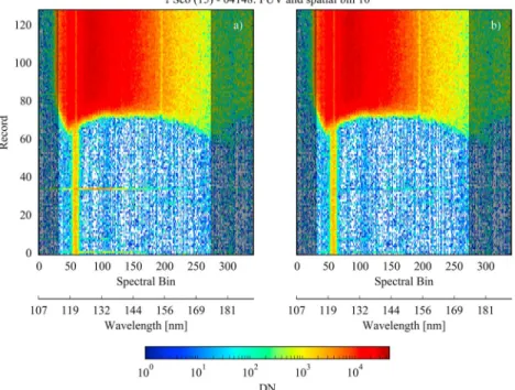
A cosmic ray event is a noticeable spike in the signal that covers a broad wavelength region. Figures 2a and 2b show raw occultation data, corrected only by dark current subtraction, before and after cosmic ray removal. To correct the spectrum for cosmic rays, the light curve L for each spectral and spatial bin is fitted by a function of the form L(r) = exp ( − exp ( −∑ n an(r − r0)n )) , (1)
where r equals the altitude (record) and r0and anare the exponential coefficients. This correction is needed to
determine the altitude where the stellar signal is no longer present. The signal at these altitudes is important for the removal of background due to atmospheric emissions. A cosmic ray event is found when the normal-ized signal is higher than 0.75% at altitudes where the signal is already completely absorbed. This threshold was retrieved with an empirical approach, finding the right balance between the correction of cosmic ray events but avoiding correction of random noise in the spectrum. The cosmic ray correction is only applied to altitudes where the stellar signal is completely absorbed.
3.2.3. Atmospheric Emission Correction
In addition to the stellar signal, the IUVS occultation data contains nonnegligible signals from atmospheric emissions of H Lyman𝛼 at 121.6 nm and OI emissions at 130.4 and 135.6 nm. The main entry ways for this contamination are the keyholes at the end of the IUVS slit. Because the emissions are spatially extended and the keyholes wider than the IUVS slit, the recorded lines are broad and contaminate sizable spectral regions centered on the wavelengths of the spectral lines. Figure 3 shows that the H Lyman𝛼 airglow contamination is easily recognized as a trapezoidal shape (black dash-dotted line) underlying the narrower stellar signal. In order to separate the actual stellar signal and the contamination due to the airglow, we model the spatial distribution of the signal as the sum of a Gaussian profile for the stellar signal and a trapezoidal pedestal for the atmospheric emissions. We use data within 2 standard deviations of the center of the Gaussian profile
Figure 2. The recorded FUV spectrum of𝜏Sco executed on 16 November 2016 at 23:50:50 (orbit 04148) for spatial bin 10. (a) The uncorrected spectrum where two cosmic ray events can be seen; one event at record number 35 and a less pronounced event below the limb at record number 1. (b) The cosmic ray corrected version of the spectrum. The gray shaded areas on both sides of each image are not used for the retrieval process. FUV = far ultraviolet.
to extract the stellar signal. The spatial size of the pedestal is correlated with the keyhole and ranges from spa-tial bins 19 to 36 for the large keyhole and from 5 to 15 for the small keyhole. The atmospheric emissions are present at all altitudes. We assume that they are constant with altitude and calculate a mean value over alti-tudes where no stellar signal is detected and subtracted this from the signal. Figure 4 shows an example of the original and corrected light curve near H Ly-𝛼. Removal of atmospheric emissions is essentially a downward displacement of the light curve.
Figure 3. H Lyman𝛼contamination of the signal for𝜆Sco executed on
26 March 2015 at 11:48:21 (orbit 00943) as a function of detector spatial bin for the spectral bin centered at 121.25 nm. Altitude is coded by color with blue colors represent lower altitudes and red colors higher altitudes. The vertical blue dash-dotted lines indicate the 2𝜎standard deviation of the central, Gaussian-like peak. Our model for the contribution of atmospheric emission to the signal is illustrated by the black dash-dotted line.
3.2.4. Stray Light Correction
Observations made of the dayside or near the relatively bright terminator are often contaminated with stray light with a spectral shape consistent with the solar spectrum scattered from Mars. This stray light is a serious problem for dayside MUV occultations. It also plagues FUV occultations through first-order MUV emissions, which show up in the FUV, albeit at a greatly reduced level. In fact, this stray sunlight usually only causes prob-lems in the FUV channel if the MUV detector is saturated by stray light, because this prevents us from using the MUV signal to correct the FUV sig-nal. Algorithms to remove the stray light contamination are under devel-opment. For the data analyzed here, we correct a small number of FUV occultations for which the stray light appears only in the altitude regions where the FUV starlight is fully attenuated. This allows us to examine many dayside occultation measurements.
3.3. Calculation of the Transmission Spectrum
In order to analyze atmospheric absorption, we define a transmission spectrum Ti,jfor the jth spectral bin and the ith LOS as
Ti,j= S(zi, 𝜆j)∕S0(𝜆j), (2) the ratio of the attenuated spectrum, S(zi, 𝜆j), to a reference spectrum,
S0(𝜆j), obtained as the average spectrum at altitudes where attenuation
is negligible. For a typical occultation, absorption signatures are present up to ∼160 km; therefore, we use the regions above 180 km to define
Figure 4. Measured and atmospheric emission corrected light curve for𝜆Sco executed on 24 March 2015 at 23:43:54 (orbit 00935) in red and green, respectively, for a wavelength of 121.57 nm.
the reference spectrum. A single stellar occultation takes between 3 and 13 min, with a mean duration of 5:30 min, and thus, attenuated and reference spectra are recorded nearly at the same time and changes stellar output or instrument response due to temperature variation, sensitivity drift, etc., are negligible.
We adopt an empirical approach to determine the errors in the transmission spectrum. We measure the time variation of the signal in the unattenuated region of the occultations assuming that these variations repre-sent random measurement errors. We further assume that the errors are independent of wavelength. This allows us to determine the dependence of random uncertainty on signal strength. Figure 5 shows the standard deviation divided by the mean versus the signal. Errors are calculated individually for each occultation using this technique.
3.4. Fitting the Transmission Spectrum
The next step in the analysis is to fit the transmission to determine the LOS column abundances for the absorb-ing species. The absorption of the stellar irradiance F0(𝜆) by the atmosphere along the LOS, between the star and the IUVS instrument, can be described via the Beer-Lambert law:
F(𝜆, z) = F0(𝜆)e−𝜏(𝜆,z) (3)
Figure 5. Relative standard deviation (standard deviation divided by the mean) depending on the signal for𝜂Cen
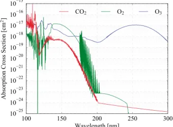
Figure 6. CO2, O2, and O3absorption cross sections used for the spectral inversion.
with𝜏 the optical depth, related to LOS column abundances by
𝜏(𝜆, z) = Σk𝜎k(𝜆)Nk(z) +𝜏𝜆0 (𝜆 0 𝜆 )𝛼 , (4)
where Nkis the LOS column density of the kth species and𝜎kits absorption cross section, assumed constant along the LOS. Based on previous results and visual examination of the spectra, we consider only absorption due to CO2, O2, and O3. The last term in equation (4) represents extinction by aerosols, which is modeled by
a simple power law dependence on wavelength. The exponent𝛼 is referred to as the Angström coefficient (Dubovik et al., 2000; Montmessin et al., 2006). Absorption by CO2, O2, and O3shows distinctive absorption
features (cf. Figure 6), but extinction due to aerosols is smooth and affects the whole wavelength range. LOS column abundances for each tangent altitude are determined by fitting the measured data with a model for the transmission spectrum using the Levenberg-Marquardt algorithm. The model transmission for the jth LOS in wavelength bin𝜆iis calculated through
i,j = ∫ d𝜆′R(𝜆′, 𝜆 i)F(𝜆′, zj) ∫ d𝜆′R(𝜆′, 𝜆 i)F0(𝜆′) , (5) where R(𝜆′, 𝜆
i) is the instrument line spread function. The integrals in equation (5) are carried out at a
reso-lution of 0.08 nm to accurately account for the high-resoreso-lution structure in the absorption cross sections and solar spectrum.
The uncertainties of the fitted parameters are obtained directly from the Levenberg-Marquardt algorithm as the square root of the diagonal terms of the returned covariance matrix. A Monte Carlo approach was used to check this procedure. We generated 500 synthetic transmission spectra, varying around the original transmis-sion spectrum assuming a Gaussian distribution of errors with a standard deviation determined from Figure 5. Each synthetic transmission spectrum is fit in the same manner as the original data, resulting in a distribution of the fitted parameters. The standard deviation of this distribution provides an estimate of the uncertainty in the fit parameters, and it is in agreement with the uncertainties delivered by the Levenberg-Marquardt algorithm. We use the latter because the Monte Carlo approach is computationally burdensome.
We analyze the FUV and MUV transmission simultaneously because CO2absorption is seen in both channels.
We have found that the optimal way to combine the two regions is to use the FUV spectrum up to 175 nm and the MUV spectrum for wavelength longer than 175 nm. This means ignoring the FUV signal between 175 and 190 nm. We determined empirically that inclusion of these data did not improve results, likely because of the low signal-to-noise ratio (SNR) in this region of the FUV channel.
Absorption cross sections for the spectral inversion are needed to fit the CO2, O2, and O3abundances. We
assumed a mean temperature in the Martian atmosphere of 180 K, and the absorption cross sections closest to the available temperature are used. The cross sections are shown in Figure 6. The CO2absorption
Table 2
Photoabsorption Cross Sections
Wavelength range (nm) Temperature (K) Reference CO2
89.03930–109.89010 195 Archer et al. (2013) and Stark et al. (2007) 109.89560–118.70130 195 Stark et al. (2007)
118.70390–163.37020 195 Yoshino et al. (1996) 163.37300–192.48810 195 Parkinson et al. (2003) 192.48970–199.98835 295 Parkinson et al. (2003)a
200.00000–201.58000 298 Ityaksov et al. (2008)b
200.00000–320.00000 — Huestis and Berkowitz (2011) O2
100.00000–107.70000 298 Matsunaga and Watanabe (1967) 107.97441–108.70008 295 Wu et al. (2005)
108.75000–114.95000 298 Ogawa and Ogawa (1975) 115.00000–132.00000 303 Lu et al. (2010)
132.04000–175.24000 295 Yoshino et al. (2005) 175.43860–204.07954 130–500 Minschwaner et al. (1992) 194.00000–240.00000 298 Yoshino et al. (1988, equation 3) 240.88843–244.99820 287–289 Fally et al. (2000)
245.00000–320.00000 — set to zero (above the dissociation limit) O3
99.0000–108.5000 295 Ogawa and Cook (1958) 110.1510–184.6484 295 Mason et al. (1996) 184.9223–213.3341 195 Yoshino et al. (1993) 213.3400–320.0000 193 Serdyuchenko et al. (2014)
aShifted by a factor of 0.45 to adopt for the different temperature.bUsed the Rayleigh scattering corrected cross sections
and shifted by a factor of 0.45 to adopt for the different temperature.
at 120.6 and 124.6 nm and O2absoprtion in the Schumann-Runge continuum alters the slope of the
spec-trum in the 140- to 160-nm region. Ozone shows a distinctive feature in the Hartley bands, a broad absorption feature centered around 255 nm. Thus, O2absorption is detected in the FUV channel, O3in the MUV channel,
and CO2in both.
Several sources have been combined to get the CO2absorption cross section over the wavelength range
from 100 to 300 nm. Rayleigh scattering by CO2is included for wavelengths longer than 202 nm. A composite absorption cross section for O2is used again to cover the wavelength range. When available we used cross
sections measured at a temperature of 195 K. The O3absorption cross section shows no temperature
depen-dence in the wavelength range of interest. Table 2 shows the sources for the cross sections along with the wavelength range and temperature range of the measurements. A detailed description of the temperature sensitivity of the retrieval process can be found in Sandel et al. (2015).
Figure 7 shows a sample of a measured transmission spectrum for the combined FUV and MUV channels at two different altitudes and the corresponding best fit transmission. The separate contribution of CO2, O2, and O3and aerosols is also shown. Shaded areas represent the uncertainties obtained from the fitting algorithm.
In panel (a), at an altitude of around 30 km, the O2column density is tied to 2×10⁻³of the CO2column density.
In panel (b), at around 110 km, no contribution due to aerosols and ozone can be seen and their transmission is unity. At 30 km, significant absorption can be seen around 250 nm due to ozone. Furthermore, a decrease of the transmission spectrum over the whole wavelength range due to the aerosols (orange line) can be noticed. In this example around 30% of the stellar signal gets absorbed by aerosols. In contrast, the transmission at 110 km shows no absorption due to ozone and aerosols. The main contribution to the absorption in the FUV
Figure 7. Transmission spectrum of the combined far ultraviolet and mid-ultraviolet channels for𝛾1Vel executed on 17 March 2016 at 12:40:25 (orbit 02848)
and two different altitudes at around 30 and 110 km, panels (a) and (b), respectively; measurements including their uncertainties in black and the best fit in red with the reduced chi-square𝜒2
𝜈. The contribution of CO2, O2, and O3including their fitted column densities and from the aerosol to the fitted transmission
spectrum are shown in green, light blue, blue, and orange, respectively. Shaded areas covering the fitted transmission spectra represent the uncertainties obtained from the fitting algorithm. The lower panels show the residuals between the measured and the modeled transmission spectra. The residual is calculated as the difference between the measured and the fitted transmission divided by the measured transmission uncertainty.
wavelength range is due to CO2and O2. As one can see, the absorption in the Schumann-Runge continuum
of O2affects the slope near 150 nm. Moreover, two sharp O2bands at 120.6 and 124.6 nm produce distinctive
features that can be seen on the low wavelength side of the CO2absorption band.
We obtain best results by fitting the spectra in three steps: determine (1) the wavelength shift, (2) the O2 abundance, and (3) the CO2and O3abundances together with the aerosol optical depth and the Angström
coefficient. We determine the wavelength shift using only the FUV channel as it has sharper spectral features than the MUV. This is permissible because the FUV and MUV spectral shifts are affected in the same way by spacecraft pointing. We fit the tranmission spectrum at each altitude with the CO2and O2column densities
and the wavelength shift as free parameters. The initial guess for the wavelength shift is determined empir-ically from comparison of the data to synthetic transmission spectra, relying on the distinctive absorption features in the molecular cross sections. Fits are applied only where CO2is not saturated (> ≈100 km). As
shown in Figure 8, the derived wavelength shifts for low SNR occultations display point-to-point variations, which must be noise rather than oscillations of the spacecraft. For occultations with high SNR the wavelength shifts derived from these fits are much more constant with altitude than for occultations with lower SNR (Figure 8). We therefore assume that the wavelength shift is constant with altitude within an occultation and set it equal to the mean value of the fit results. This wavelength shift is held constant in subsequent steps. Next, we consider the O2distribution in the atmosphere. O2is only detectable in the FUV spectral region
and at high altitudes, typically above ∼90 km. In this step, we keep the CO2and O2column densities as free
parameters but fix the wavelength shift to the constant value that was obtained in the first step. The O2column densities determined in the fits appear reasonable but are sometimes noisy, and moreover, the O2noise can induce noise in the retrieved CO2column density. Physically, we expect the O2/CO2ratio to vary smoothly with
Figure 8. Spectral shifts for four different occultations. The solid lines show
the actual fitted value including the uncertainties. The dash-dotted lines indicate the constant wavelength shift used in the analysis.
density with the fit (Figure 9). The fit is extended downward until the ratio of O2to CO2column densities reaches a value of 2 × 10⁻³, below which
the ratio is set equal to this value. As shown in Figure 9, the power law pro-vides an excellent fit to the observations. The increase in the O2/CO2ratio
with altitude is expected because O2is created by photochemistry at high
altitudes and is lighter than CO2and therefore enhanced at high altitude
by diffusive separation, but here we simply treat the O2mixing ratio model as an empirical fit to the data. The asymptotic ratio of 2 × 10⁻³is
consis-tent with the bulk of the occultation results but is not necessarily correct for any individual occultation. This has little affect on our results because the occultation is no longer sensitive to O2density as long as it is of order
10−3. The procedure described above works for O-type stars and B-type
stars down to the subclass B3. However, for cooler stars, B-type stars with a subclass number higher than B3 and A-type stars, the retrieval of the O2is not included because stellar emission is too weak in the wavelength region containing the distinctive O2features. Therefore, for IUVS stellar occulta-tions targeting𝛼 Gru (B7), 𝛼 Lyr (A0), 𝛽 Tau (B7), 𝛼 Leo (B7), and 𝛼 And (B8) we simply confine the wavelengths analyzed to longer than 126 nm and fix the O2/CO2column density ratio at 2 × 10⁻³and fit for only CO2, O3, and
aerosols.
The third and final fit is performed with the constant wavelength shift and the smooth O2profile determined
in the earlier steps. This fit determines the CO2and O3column density profiles, the aerosol optical depth at
a reference wavelength of 250 nm, and the Angström coefficient. The full set of results for an occultation of
𝛾1Vel is shown in Figure 9. 3.5. Vertical Inversion
Local number densities are obtained from the LOS column densities by a vertical inversion. Our approach is based closely on that described in Quémerais et al. (2006), but we have made a number of significant improvements and therefore present a complete description of the algorithm currently in use.
Figure 9. Results of spectral fits to the𝛾1Vel occultation executed on 17 March 2016 at 12:40:25 (orbit 02848).
(a) The retrieved column densities for CO2(red), O2(green), and O3(blue). The dash-dotted lines indicate the original fit (O2column density free to vary), whereas the solid lines show results with the with a fixed value for the ratio of O2to CO2column density. (b) The dash-dotted line shows the O2/CO2column density ratio from the spectra fits, and the solid line shows the smoothed profile used in the fits of CO2, O3, and aerosols. (c) The retrieved aerosol optical depth𝜏at 250 nm and the Angström coefficient𝛼are shown in orange and brown, respectively.
The LOS column density Njis the integral over the local number density n along the LOS. Assuming spherical symmetry, we have Nj= 2 ∫ +∞ aj n(r)√ r r2− a2 j dr (6)
with ajas the radius distance of the lowest point along the LOS to the center of Mars, r the radius distance to a point in the atmosphere, and n(r) as the local number density at that point. Dividing the atmosphere into discrete layers, this expression can be written in matrix notation as
N = K⋅ n, (7)
where N represents the vector containing the Njvalues and n the vector of the local number densities at the center of the layers. The K matrix represents the LOS integration:
Kji= 2 ∫ ri+1∕2 ri−1∕2 f (r)√ r r2− a2 j dr, (8)
where i indicates the atmospheric layer and j the LOS. The function f (r) gives the variation of the local number density in the layer. We assume that f (r) = 1, which is accurate for sufficiently thin layers.
According to equation (8) in Quémerais et al. (2006) an estimator for the local number density n0can be obtained by
n0= Sn0K
⊺S
e−1N, (9)
where Sn0is the covariance matrix associated with this estimator given by
Sn0 = (
K⊺Se−1K
)−1
. (10)
Seis a diagonal matrix with elements equal to the square of the standard deviation𝜎iassociated with the
slant column density Niobtained from the spectral inversion:
( Se ) ij=𝜎 2 i𝛿ij. (11)
The uncertainties ffin0of the retrieved number densities n0are calculated from Sn0via
(𝛿n0)i=√(Sn0 )
ii. (12)
In most cases, the solution described above causes an amplification of the noise. Quémerais et al. (2006) used the Tikhonov regularization method (Tikhonov & Arsenin, 1977; Twomey, 1977) to lessen this effect. This is done by including a smoothness constraint to the inversion:
n = SnK⊺Se−1N, (13) where Snis given by Sn= ( K⊺Se−1K + L⊺Ss−1L )−1 (14) with Ssdefined by Ss−1=𝜆sI = ⎛ ⎜ ⎜ ⎜ ⎜ ⎜ ⎜ ⎜ ⎝ 𝜆s1 0 0 · · · 0 0 0 0 𝜆s2 0 · · · 0 0 0 0 0 𝜆s3 · · · 0 0 0 ⋮ ⋮ ⋮ ⋱ ⋮ ⋮ ⋮ 0 0 0 · · · 0 𝜆sk−1 0 0 0 0 · · · 0 0 𝜆sk ⎞ ⎟ ⎟ ⎟ ⎟ ⎟ ⎟ ⎟ ⎠ , (15)
Figure 10. (a–d) Number density profiles for𝜂UMa executed on 1 August 2015 at 15:09:17 (orbit 01635) using different smoothing coefficients𝜆0= 0.05, 0.10, 0.20, and 0.30 for the Tikhonov regularization. The gray line in panel (b) represents the column number density.
and L defined by L = ⎛ ⎜ ⎜ ⎜ ⎜ ⎜ ⎜ ⎜ ⎝ −1 1 0 0 · · · 0 0 0 0 1 −2 1 0 · · · 0 0 0 0 0 1 −2 0 · · · 0 0 0 0 ⋮ ⋮ ⋮ ⋮ ⋱ ⋮ ⋮ ⋮ ⋮ 0 0 0 0 · · · 0 1 −2 1 0 0 0 0 · · · 0 0 1 −1 ⎞ ⎟ ⎟ ⎟ ⎟ ⎟ ⎟ ⎟ ⎠ . (16)
L represents a discrete second derivative operator in the interior of the domain and a first derivative operator
on the boundaries. In our case, this operator is not divided by the squared distance between two consecutive layers as mentioned in Quémerais et al. (2006), because this effect is incorporated in the smoothing parameter
𝜆0, discussed below.
The right choice for the smoothing coefficient is a compromise between two aspects, the smoothness and the altitude resolution. Using a low smoothing coefficient gives a poor regularization and results in a noisy number density profile but with an good altitude resolution. Alternatively, choosing a high smoothing coefficient gives a smooth profile but decreases the altitude resolution. Quémerais et al. (2006) obtained good results when the smoothing constraint varies with altitude according to
𝜆si(r) =𝜆0
1
𝛿n2
i
, (17)
with the single smoothing coefficient𝜆0, adjustable to balance smoothness and altitude resolution. We
adopt this approach here. Figure 10 shows the effect of different values of𝜆0on n. We discuss further the
consequences of different choices of𝜆0in the next section.
With this approach, it is necessary to solve for the number densities iteratively because the smoothing coefficients used to derive the number densities also depend upon the number densities, through their uncertainties. The first iteration is without any smoothing to get an estimator for the local number densities and their uncertainties using equations (9) and (10). In the following iterations the Tikhonov regularization, equations (13) and (14), are used and the new errors for the next iteration are calculated. Iterations are continued until convergence satisfies a specified tolerance:
max (| || || k+1n i−kni) kn i || || | ) ≤ 𝜖, (18)
In section 4.5 we interpret wave-like perturbations of the CO2number density profile as tides in the ther-mosphere. This interpretation rests on the conclusion that the observed perturbations are a property of the atmosphere rather than an instrumental or data reduction artifact. We present the arguments in support of this assertion in this section.
Tikhonov regularization represents a smoothing of retrieved densities, and therefore, there is a danger that noise in the data will be spread over several data points by the regularization process and will thus appear as a real feature when it is simply an artifact created by noise combined with smoothing. To demonstrate that this is not the case for the perturbations seen in the densities retrieved from the occultations, we show in Figure 10 both the column density and the local density from a typical occultation. It is clearly seen in Figures 10a and 10b that the wave-like perturbations are present in the column densities, and furthermore, the perturbation amplitudes are not amplified in the inversion process.
On the other hand, we must also be careful that the smoothing in inversion process does not damp or remove real perturbations. To investigate this, we have looked at results obtained with several values of the smoothing coefficient. Figure 10 shows local densities obtained with smoothing coefficients of𝜆0= 0.05, 0.10, 0.20, and 0.30. With𝜆0= 0.20 and 0.30 the wave feature seen in the local density are smoothed out, albeit only slightly, implying that some information on wave structures has been lost. With a smoothing coefficient of𝜆0= 0.10
and 0.05, the wave structures are preserved. Using values lower than 0.10 in the iteration does not lead to substantially different density profiles. Thus, a smoothing coefficient𝜆0= 0.10 is used for all results presented
in this study with an altitude sampling less than 6 km. However, for an altitude spacing higher than 6 km a𝜆0
value of 0.01 is used.
We have investigated several other possible sources of artifacts in the local density profiles. For example, when developing our data reduction algorithm, we noticed that noise in the derived wavelength shifts and O2densities cause perturbations in the CO2densities. The procedures described in the previous sections to treat wavelength shifts and O2densities were designed in part to remove these artifacts. Another possible artifact could result from periodic variations in spacecraft pointing that might then appear as a wave in the retrieved column densities. To investigate this, we have compared both wavelength shifts and spacecraft pointing information with the observed perturbations and have not found any correlation (see Figure 8). Thus, we conclude that wave-like perturbations in the derived local densities represent a real characteristic of the Mars atmosphere.
3.6. Calculation of the Temperature
As the dominant constituent in the atmosphere, the CO2distribution is in hydrostatic equilibrium and analysis
of the density profile can be used to determine the atmospheric temperature. The technique used here to derive temperature profiles follows that described by Snowden et al. (2013). The partial CO2pressure at an
altitude riis calculated by integrating the hydrostatic equilibrium from the upper boundary r0down to rias
P(ri) = P(r0) + mCO2
r0
∫
ri
nCO2(r)g(r)dr, (19)
where nCO2(r) is the smoothed CO2number density, g(r) the acceleration of gravity, mCO2the molecular mass of CO2, and P(r0) the pressure at r0, the upper boundary. The temperature T(r) is calculated from the ideal
gas law:
T(r) = P(r)
kBnCO2(r), (20)
with kBBoltzmann’s constant. The CO2number density used in equation (19) has been smoothed using a mod-ified Savitsky-Golay filter with a five-point sliding window in order to damp small scale fluctuations (Snowden et al., 2013).
The pressure at the upper boundary P(r0) is determined by fitting the measured density above r0to the
expres-sion for a hydrostatic variation with a constant temperature gradient (Snowden et al., 2013). Typically, we set the upper boundary of the temperature calculations at the altitude for a transmission of 0.95 at 150 nm although for bright stars we find that we can extend the analysis to the altitude where the transmission is 0.98.
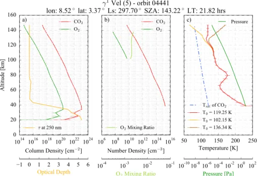
Figure 11. Results obtained during the whole retrieval process for𝛾1Vel executed on 12 January 2017 at 05:32:50 (orbit 04441): fitted column densities and the optical depth𝜏at 250 nm (panel a), inverted number densities and the O2 mixing ratio (panel b), and the temperature and pressure profiles (panel c). The temperature profiles in orange, red, and brown represent the different upper boundary temperaturesT0. The blue dash-dotted line in panel (c) indicates
the CO2saturation temperature.
in this region is unknown, we consider values of zero gradient (isothermal) and plus-minus half the adiabatic lapse rate to estimate the uncertainty due to the upper boundary condition.
A Monte Carlo approach is used to determine the uncertainties in the temperature profiles caused by uncer-tainties in the number densities. We generate 1,000 synthetic density profiles consisting of random densities chosen as elements of a normal distribution with the measured density and its uncertainty defining the mean and standard deviation of the distribution. For each of the synthetic density profiles the corresponding tem-perature profile is calculated resulting in a distribution of the temtem-perature at each altitude. The temtem-perature uncertainty is set equal to the standard deviation of this distribution.
Figure 11 shows an example of results obtained during the retrieval process from the column densities and the aerosol optical depth𝜏 (panel a), to the local number densities and the O2mixing ratio (panel b), to the
temperature and pressure profiles (panel c). The temperature profiles show the effects of the different upper boundary temperatures discussed above.
Figure 12. Retrieved CO2, O3, and O2number density profiles for stellar
occultations taken with the Imaging UltraViolet Spectrograph instrument during the first 12 stellar occultation campaigns. Colors represent different solar longitudesLsas indicated in the legend. The corresponding campaign number is given in parentheses.
4. Results and Discussions
In the previous sections we described the execution of stellar occulta-tions with the MAVEN/IUVS instrument and explained the steps necessary to retrieve number densities and temperature profiles from the measure-ments. In this section, we provide some initial results. We focus on CO2, O3, and O2number densities, temperature profiles, and perturbations seen in the CO2altitude profiles. We do not discuss aerosol and dust profiles
in detail in this paper. The data used in this section are archived in the Planetary Atmospheres Node of the Planetary Data System; we used ver-sion 13. We compare our measurements with values determined from previous observations as well as with predicted profiles from the Mars Climate Database (MCD) v5.2. The MCD is derived from the Laboratoire de Météorologie Dynamique Mars Global Climate Model (LMD-MGCM, Forget et al., 1999) extended in the upper atmosphere as described
Figure 13. Solar longitude dependence of the CO2number density at 100 km. Colors represent the number densities for a different stellar occultation campaign (listed in Table 1). The solid red line shows the sinusoidal least squares fit to the measured densities. In addition, the CO2 number densities from Mars Express/SPICAM stellar occultations shown in Forget et al. (2009) are included as gray open circles. The Imaging UltraViolet Spectrograph and SPICAM data shown here include measurements at latitudes below 50∘and all available longitudes and local times. SPICAM = Spectroscopy for Investigation of Characteristics of the Atmosphere of Mars.
in González-Galindo et al. (2009, 2015) and includes a photochemical model able to simulate the O3cycle (Lefèvre et al., 2004, 2008). The MCD
contains model output averaged over a Mars month (intervals of 30∘ of Ls, typically 50–60 sols) at 12 local times. The MCD output covers the entire atmosphere of Mars from the surface to ∼250 km with an altitude resolu-tion that ranges from 4 km in the lower atmospheres to 8 km in the upper atmosphere. A horizontal 64 × 49 grid is used for the longitude and lati-tude resolution in the MCD, resulting in a 5.625∘ sampling in the longilati-tude and a 3.75∘ sampling in the latitudinal direction. An overview of the MCD version 5 used here can be found in Millour et al. (2014). The MY covered by MAVEN/IUVS stellar occultations is not yet included in the MCD database; thus, we used the available MY that has an F10.7index (solar radio flux at
10.7 cm at 1 AU) that is closest to that at the time of the occultations; MY26 for campaign 1 and 2, MY27 for campaigns 3–7, and MY28 for campaigns 8–10. Although MY28 was closer to the F10.7, index for campaigns 11 and 12, we used MCD MY29 output for these campaigns, as they occurred at times of year with a major global dust storm in MY28.
4.1. CO2Density
A survey of the CO2density in the upper mesosphere/lower thermosphere
of Mars is a main goal of the analysis conducted here. As the main atmo-spheric component, its density and temperature are key parameters to understand the processes at play in the region of the atmosphere where a number of characteristic processes interact (radiative cooling, dynamics, molecular decomposition, etc.) and where couplings between the lower and the upper atmosphere can be identified. In particular, the role of gravity wave propagation and dissipation and the associated deposition of momentum are still only tenta-tively understood. Their impact on the mean upper atmospheric circulation remains to be demonstrated by observations, one objective that guides the analysis presented in this investigation. In addition, improving our knowledge of CO2 density/temperature and its seasonal/spatial variability in the altitude range cov-ered by IUVS will provide engineers with the information needed to prepare the future of Mars’ exploration (aerobraking, Entry/Descent/Landing phases).
Figure 12 shows the CO2, O3, and O2number density profiles as a function of pressure. It is convenient to use the pressure scale to compare the retrieved number densities, as it compensates for temperature differences at lower altitudes. The variation in density at a constant pressure is up to a factor of 3 for CO2. Because the
atmosphere is an ideal gas, the variability in density at constant pressure is due to variability in the local tem-perature. The variation in O3and O2is much larger, up to an order of magnitude at some pressures for O2and
even higher for O3.
Figure 13 shows the variation of CO2number density with Lsat an altitude of 100 km along with the CO2
number densities derived from SPICAM occultations (Forget et al., 2009). The variation with Lsis similar for
the IUVS and SPICAM results but the densities reported here have a higher variability at a given Ls. Although the occultations from the IUVS and the SPICAM instrument are 10 years apart, solar activity as measured by the F10.7index (solar radio flux at 10.7 cm) are comparable. Furthermore, the National Oceanic and
Atmo-spheric Administration Mg II core-to-wing ratio, derived from the solar Mg II feature at 280 nm, which is a good measure of solar UV and extreme ultraviolet emissions (Viereck & Puga, 1999; Viereck et al., 2001), shows comparable values for both time frames.
The SPICAM data show a sudden increase of the CO2number density at Ls∼ 130∘ (Forget et al., 2009). During
this time, Spirit and Opportunity, the two Mars Exploration Rovers, measured a significant and unusual rise of dust opacity, which affected most of the planet (Smith et al., 2006). This increase in optical depth was enough to increase the temperature in the lower atmosphere, thereby raising densities in the upper atmosphere (Forget et al., 2009). However, there are also seasonal variations separate from dust storm influences. Campaign 7 was executed at Ls ≈ 124∘, shortly before the Lsof ≈ 130∘ at which the storm commenced in MY27, and campaign 8 occurred at Ls ≈ 159∘. Unfortunately, there are no data from the MUV channel
for this campaign, which means no CO2number densities below about 90 km. However, data from the FUV
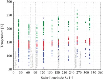
Figure 14. The temperatures required to explain the density variations
at 120 km shown in Figure 13. Surface temperatures from the Mars Climate Database are shown in green, temperatures at 120 km inferred from Imaging UltraViolet Spectrograph occultations are shown in blue, and the mean temperature between the surface and 120 km is shown in red.
as in the SPICAM data, especially at Ls ≈ 159∘. Moreover, the IUVS CO2
number densities from campaign 9, Ls≈ 186∘, are still slightly lower than the SPICAM values. This suggests that the sharp increase in the SPICAM data near Ls = 130∘ was due to the dust storm and furthermore that the atmosphere during MY27 remained dustier than during MY33 until at least Ls= 186∘.
Because the atmosphere is in hydrostatic equilibrium, the variability in CO2
density at a constant altitude reflects temperature variability at lower alti-tudes as well as possible variations in the surface pressure. The average temperature in the lower atmosphere can be calculated from hydrostatic equilibrium: ⟨1 T ⟩−1 = −GM Rd r0− r1 r0r1 ( ln (p 1 p0 ))−1 , (21)
where G is the gravitational constant, M the mass of Mars, Rdthe specific
gas constant, r0and r1the radial distances to the surface and 120-km level
along the direction of gravity, and p0and p1the surface pressure and
pres-sure at 120 km. Because p0is not measured in the occulations, values are
taken from the MCD for the same geometry as the occultation and for the MY closest in solar flux to the actual flux of the occultations. As mentioned earlier, altitudes used here are relative to the Mars reference ellipsoid, but the MCD altitudes are relative to the areoid (Mars geoid). Thus, to get a comparison in the same altitude space, the MCD altitudes are adjusted to the ellipsoid using a smoothed topography map (based on a 1∘ × 1∘ Mars Orbiter Laser Altimeter map). The altitude shift is between −2.52 and 1.12 km. Results for the mean tem-perature are shown in Figure 14. The observed density variation at 120 km can be explained by a seasonal variation in mean temperature from 140 to 160 K.
4.2. O3Density
Ozone on Mars exhibits orders of magnitude variations in space and time as a consequence of photoly-sis, atmospheric dynamics, and the catalytic destruction cycles induced by hydrogen radicals (HOx) released
by dissociation of H2O (Lefèvre & Krasnopolsky, 2017). An anticorrelation between O3and H2O is therefore
believed to take place in the atmosphere of Mars, and this has been confirmed by spacecraft and Earth-based observations of Mars. As such, O3testifies to the oxidizing properties of the Martian atmosphere and returns
direct information on the mechanisms at work in controlling the stability of the present-day CO2atmosphere.
Ozone is detected only in the MUV channel and only in those occultations that are relatively free of scat-tered light. This effectively limits O3measurements to nightside occultations. Moreover, in some occultations, extinction by aerosols is so large that it masks the O3signature. In all, we estimate that we have 163
occulta-tions in which O3could be detected if it were sufficiently abundant. We detect O3in 70 of these occultations
and estimate an upper limit for the remaining 93 occultations. We can measure O3for LOS column densities
greater than ∼1015cm−2. Examination of the full set of occultations shows that this upper limit is surprisingly
independent of the SNR of the occultation. The peak number density corresponding to this column density limit is ∼107cm−3. We discuss here results from a subset of the observations, concentrating on 18 occultations
that yield good altitude profiles of O3. Table 3 lists the occultations. Our selected observations come from
campaigns 3, 5, and 7. These three campaigns are separated by 3 to 4 Earth months, and thus, each campaign represents a different season on Mars: campaign 3 (Ls≈ 21∘) was executed during early fall in the southern hemisphere (SH), campaign 5 (Ls ∼ 63∘) during late spring in the NH, and campaign 7 (Ls ≈ 124∘) during midwinter in the SH.
The O3density profiles for the occultations listed in Table 3 are shown in Figure 15 and compared with the
predicted ozone profiles from the MCD. The left panels show the altitude dependence and the right panel the pressure dependence. We show both because altitude is the quantity directly related to the measurements but pressure is more directly related to physical processes in the atmosphere. The pressure corresponding to the O3measurement is determined from the CO2density and temperature inferred for that altitude. The retrieved O3profiles are generally confined to the ∼20- to 60-km region because aerosols usually obscure