Ensemble methods for APS in-flight particle temperature and velocity prediction considering torch electrodes ageing

Publisher’s version / Version de l'éditeur:

Vous avez des questions? Nous pouvons vous aider. Pour communiquer directement avec un auteur, consultez la première page de la revue dans laquelle son article a été publié afin de trouver ses coordonnées. Si vous n’arrivez pas à les repérer, communiquez avec nous à PublicationsArchive-ArchivesPublications@nrc-cnrc.gc.ca.

Questions? Contact the NRC Publications Archive team at

PublicationsArchive-ArchivesPublications@nrc-cnrc.gc.ca. If you wish to email the authors directly, please see the first page of the publication for their contact information.

https://publications-cnrc.canada.ca/fra/droits

L’accès à ce site Web et l’utilisation de son contenu sont assujettis aux conditions présentées dans le site LISEZ CES CONDITIONS ATTENTIVEMENT AVANT D’UTILISER CE SITE WEB.

International Thermal Spray Conference 2021, 2021-05-24

READ THESE TERMS AND CONDITIONS CAREFULLY BEFORE USING THIS WEBSITE. https://nrc-publications.canada.ca/eng/copyright

NRC Publications Archive Record / Notice des Archives des publications du CNRC :

https://nrc-publications.canada.ca/eng/view/object/?id=73d9763a-c940-40f5-8a31-9c25a5c93abc https://publications-cnrc.canada.ca/fra/voir/objet/?id=73d9763a-c940-40f5-8a31-9c25a5c93abc

NRC Publications Archive

Archives des publications du CNRC

This publication could be one of several versions: author’s original, accepted manuscript or the publisher’s version. / La version de cette publication peut être l’une des suivantes : la version prépublication de l’auteur, la version acceptée du manuscrit ou la version de l’éditeur.

Access and use of this website and the material on it are subject to the Terms and Conditions set forth at

Ensemble methods for APS in-flight particle temperature and velocity

prediction considering torch electrodes ageing

Ensemble methods for APS in-flight particle temperature and velocity prediction

considering torch electrodes ageing

K. R. Yu, C. V. Cojocaru, F. Ilinca, E. Irissou

National Research Council of Canada, AST, Boucherville, Québec, Canada

Abstract

In an atmospheric plasma spray (APS) process, in-flight powder particle characteristics, such as the particle velocity and temperature, have significant influence on the coating formation. The nonlinear relationship between the input process parameters and in-flight particle characteristics is thus of paramount importance for coating properties design and quality control. It is also known that the ageing of torch electrodes affects this relationship. In recent years, machine learning algorithms have proven to be able to take into account such complex nonlinear interactions. This work illustrates the application of ensemble methods based on decision tree algorithms to evaluate and to predict in-flight particle temperature and velocity during an APS process considering torch electrodes ageing. Experiments were performed to record simultaneously the input process parameters, the in-flight powder particle characteristics and the electrodes usage time. Various spray durations were considered to emulate industrial coating spray production settings. Random forest and gradient boosting algorithms were used to rank and select the features for the APS process data recorded as the electrodes aged and the corresponding predictive models were compared. The time series aspect of the data will be examined.

Introduction

The importance of the in-flight powder particle characteristics, such as the particle velocity and temperature, on the coating formation in the complex nonlinear atmospheric plasma spray (APS) process are long well recognized. Since these characteristics cannot be measured during production, there is a great interest to predict these parameters to monitor and improve the spray process and coating quality.

Predictive models for in-flight particle characteristics

The recent advancements in machine learning algorithms make modeling such complex nonlinear interactions possible. Guessasma et al. proposed to develop an expert system using artificial neural network (ANN) models to predict the average spray particle velocity, temperature and diameter for better coating quality control [1]. Input parameters, also referred to as attributes or predictors, like arc current intensity, argon and hydrogen gas flow rate, were considered. Choudhury et al. also applied ANN to predict the in-flight powder particle characteristics of an atmospheric plasma spray process [2]. The authors proposed to expand the experimental dataset using kernel regression to improve the generalization ability of the trained ANN. Kanta et al. suggested to develop an expert system using ANN and fuzzy logic to better control the in-flight particle characteristics under the influences of different

fluctuations of the APS process [3]. Later, Choudhury et al. employed extreme learning machine (ELM), a specific class of ANN, to construct a robust single hidden layer feed forward neural network for the in-flight particle characteristics of the APS process [4]. This approach reduced the training time and yielded stable performance with regard to the changes in the number of hidden layer neurons. Choudhury et al. further proposed to implement the ANN using a modular scheme [5]. The scheme simplified the model structure and improved the generalization of the model overall.

Ensemble methods

In literature, all predictive models proposed for APS in-flight particle characteristics are based on ANN. There are however many other nonlinear predictive models, e.g. support vector machines, ensemble methods, etc. [6]. In particular, decision tree based ensemble methods, like random forest and gradient boosting, have demonstrated their strong performance, often comparable to and sometimes even better than ANN [7], [8]. The essential idea behind ensemble methods is to combine the outputs from many simple models, referred to as base learners, to yield the final prediction. Random forest and gradient boosting are two popular ensemble methods; both use decision tree as their base learners. The two differs however in how the individual trees are constructed and added together. Random forests generates the trees by training them on subsets of data, both in terms of the observations and the attributes, randomly drawn from the full training set with replacement [9]. The final prediction is an average of the results from all the generated trees. Since the trees do not depend on each other, the procedure is well suited to be executed in parallel. Random forest reduces the prediction variance. On the other hand, gradient boosting constructs each tree sequentially aiming to reduce the prediction error or the residue from the previous trees [10], [11]. Subsampling in observations are generally considered, while subsampling in attributes may also be employed [12]. Gradient boosting reduces both the prediction variance and bias.

Wolpert argues that without having substantive information about the modeling problem, there is no single model that will always do better than any other model [13]. Could ensemble methods also predict well the in-flight particle characteristics?

Time series aspect of APS data

It is well known that the ageing of torch electrodes greatly affect the relationship between the APS input parameters and the in-flight particle characteristics, in a time scale of hours. The same set of process inputs would expect to yield different in-flight particle characteristics using a brand new electrode pair as compared to a used one. Therefore, when modeling the in-flight particle characteristics with torch electrodes ageing considered, it may be imperative to consider the production data of APS as

time series; where there is an ordered temporal component in the observations of the data. To the authors’ best knowledge, this time series aspect of predictive modeling has not ever been considered in the predictive models previously proposed for the in-flight particle characteristics. Can better predictions be made if the production data of APS is considered as time series? This work aims to explore the applicability of two ensemble methods, namely random forest and gradient boosting, to predict and forecast the multivariate APS in-flight particle characteristics with the consideration of torch electrodes ageing as time series. In particular, two different time series modeling strategies are compared with the baseline approach. The paper is organized as follows: First, the electrode wearing experiment is described, followed by the data preprocessing. After, the two time series modeling strategies are compared and discussed. The paper concludes with the planned future work.

Electrode wearing experiment

APS experiments were performed to record simultaneously the spray process input parameters, the in-flight powder particle characteristics and the electrodes usage time. The experiment was carried out using a Metco 3MB APS torch with a brand new pair of electrodes, and pursued until the torch could no longer sustain the plasma. The main process parameters (e.g. torch current intensity, voltage) were monitored and recorded at a sampling rate of 1 Hertz, using an in-house built console equipment integrated in LabVIEW (National Instruments). Various spray time durations were considered for the torch usage so to emulate industrial coating spray production settings similar to those employed for thermal barrier coating (TBC) production. However, only a single set of spray parameters and a single TBC top coat powder (YSZ, Metco 204BN-S) was tested throughout the experiment. During the course of the experiment, it was aimed to maintain the net power of the torch constant by adjusting the torch current. An AccuraSpray (Tecnar, St-Bruno, Qc, Canada) diagnostic device was used to measure the in-flight particle temperature and velocity at defined time intervals.

Figure 1: 3MB torch electrode pair used for the experiment

Figure 2: APS coating porosity. Increased porosity is observed in the coating when spraying with the electrodes used for 7 hours (left) as compared to the ones used for 26 hours (right).

The electrodes began to show a weakness in sustaining a constant plasma plume and manifested plasma pulsations after about 26 hours of usage. At which point, it was decided that the electrodes reached their end of life. Figure 1 shows the 3MB torch electrode pair at the beginning and at the end of the experiment. Figure 2 shows the porosity of the YSZ coating prepared at two different moments corresponding to different torch electrodes usage states. As expected, the coating prepared with the electrodes closer to the end of their life time (right) is more porous.

Predictive modeling with ensemble methods

The data acquired from the different devices was first cleaned and then integrated based on the time stamp. For the data recorded from the APS controller (e.g. torch current intensity, voltage), only those observations when the plasma was on were considered. A total of about 2600 records with 9 attributes and 2 targets (i.e. in-flight particle temperature and velocity) were obtained right after the data fusion. Statistics of selected parameters are listed in Table 1.

Table 1: Statistics of selected parameters

Parameters Mean Standard _deviation

Torch current ( ) 487.9 63.8 Torch voltage ( ) 78.1 3.5 Raw power ( ) 37.9 3.5

Particle temperature (℃) 3297.0 218.4

Particle velocity (m/s) 128.1 3.8

Figure 3: Correlation among some selected parameters

Figure 3 shows the correlation among some selected parameters. Recall that in the experiment, only a single spray condition is considered with the net power maintained constant. Therefore, the net power and the flow of nitrogen (and similarly for several other parameters not shown) appear to have no relation to any other parameters. In particular, the particle

temperature seems to have stronger correlation with the voltage as compared to particle velocity.

Most machine learning predictive models, including random forest and gradient boosting, assume that the observations of the data are independent of each other, i.e. the data does not have any particular order. To forecast a time series using these machine learning models, it is necessary to capture the temporal order information properly as new attributes in each observation itself. There are two general approaches [14]. The first approach simply appends all the information from the considered previous time segments into the observation [15]. The time series may also be normalized [16], stationarized [17], or decomposed [18] a priori. The second approach only supplements the observation with specifically engineered and selected statistical features from the time series for the learning [14]. The first approach will be adopted here due to its simplicity. One disadvantage of this approach, however, is that the number of the attributes increases rather quickly as longer histories are desired, resulting in a higher model training cost. Therefore, it is desirable to include only the relevant parameters for the attribute augmentation.

Feature selection

Both random forest and gradient boosting provide a ranking of variable importance as the regression models are developed. They will be used to guide the useful attribute selection. The present prediction problem belongs to that of multi-targets regression, having two outputs: the particle temperature and velocity. The development of multi-target regression for random forest is more advanced [19]. There are already several implementations available from popular machine learning platforms [20], [21]. Such models also take into consideration the correlation among the targets. As for gradient boosting, multi-target regression is still under active development. A simple workaround is to build a separate predictive model per target. The correlation among the outputs are, however, ignored. Alternatively one may build a set of chained dependent models: Suppose that there are two outputs and . One first builds a model to predict with attributes ; and then one builds another model to predict with (the predicted from the first model) as well as the attributes . The performance of such approach depends upon the model construction order and the correlation among the targets. The benefit of the added complexity is not always apparent. Both ensemble methods will be used here to compare the features. The dataset is first randomly separated into two parts: 70% for training and 30% for testing.

Figure 4: Top 5 features ranked using random forest

The testing set is used to ensure the decent performance of the predictive model. The hyper-tuning parameters of the two models are set based on previous experience as follows: for random forest, the maximum number of features per tree is set to 2 and the depth of tree is left as maximum; for gradient boosting, the depth of tree is set to 2, with a learning rate of 0.1. The simpler separate model per target approach is employed. For both methods, a minimal leaf node size of 5 is considered. The top 5 features ranked using random forest and gradient boosting are shown in Error! Reference source not found. and Figure 5 respectively. The two sets of ranking are not identical, and both do not follow exactly the Pearson correlation (Figure 3). The ranking of gradient boosting seems to have better agreements with the Pearson correlations than those of random forest.

Figure 5: Top 5 features ranked using gradient boosting. One separated model is trained per target.

The ranking from the gradient boosting model for the in-flight particle velocity, though reasonable, according to the Pearson correlation, is counterintuitive, since the net power is purposefully maintained constant throughout the experiment. This underlines the importance of having the interaction among the targets considered. Therefore, in the following, only random forest will be studied with the top 5 features ranked in Figure 4.

Time series attribute augmentation

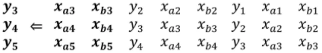
To incorporate the temporal order of the data in each observation, it is necessary to add the information of the previous observations into the present observation as new attributes. Suppose that there are two attributes: and in the original dataset for a target . The embedding procedure for a lag order of 3 results in the following data form:

⇐

where the numbers represent the ascending temporal order in the dataset. The original dataset is shown in bold. Note that the target values for the previous observations are also embedded here. For example, can be the torch current intensity and

can be the torch voltage with being the in-flight particle temperature . The embedded dataset will become as follows:

⇐

For a given dataset, a higher lag order can introduce more temporal information into the present observation. However, this will also reduce the total number of embedded observations for modeling. The tradeoff is far from trivial. For the present exploration, a lag order of 5 is considered. All the top 5 ranked features are included, resulting in 33 attributes in total in the embedded dataset, referred to as the simple embedded dataset in the following.

During data exploration, it is observed that both the targets and the attributes contain trending patterns. Hence, they are non-stationary. Traditional time series forecasting techniques will typically first use differencing to stationarize the time series data before model tuning [22]. The benefits of such data preparation for random forest is however not well reported. Therefore, a second embedded dataset, where the time series is first differenced before embedding, is prepared for comparison. This is referred to as the differenced embedded dataset below. Note that the prediction of any regression model, which is trained upon a differenced embedded dataset, requires reverse differencing to convert itself back to the original unit scale.

Methodology for forecasting experiment

A random forest regression model is developed from each embedded dataset. They are compared with a baseline random forest model developed from the original dataset, without embedding nor differencing. Since the number of attributes ( ) of these datasets are different, the number of features included per tree is set based on the rule of thumb recommended ( /3) [23], whereas the depth of tree is left as maximum as before with the minimum leaf node size of 5.

Again, the dataset is separated into two parts, according to each Accuraspray measurement record: the beginning 70% for training and the remaining 30% for testing. This arrangement emphasizes the prediction of future values.

Figure 6: The out-of-sample mean squared error versus the number of trees in the ensemble of the three random forest models

In this exploratory work, only the one-step prediction, which predicts the immediate next target value, is considered. The performance is compared using the mean square error (MSE) in the original unit scale.

Results and discussions

For each dataset, a set of random forest regression models is first constructed, with an increasing number of trees from 5 to 500. The corresponding out-of-sample MSE (i.e. against the testing data) versus the number of trees considered for the three random forest model sets are shown in Figure 6. The MSE of the simple embedded random forest model is much smaller than that of the baseline model; whereas that of the differenced embedded random forest model is substantially further reduced. For all three cases, the MSE reduces as the number of trees increases from the beginning. After certain point, a further increase in the number of trees does not reduce the MSE anymore. This transition to the error plateau provides a guideline of the required number of trees for the ensemble as per the selected hyper-tuning parameters. From Figure 6, it is indicated that the baseline random forest model needs about 300 trees. Both the simple embedded and differenced embedded random forest models (upon zoomed in) need about 200 trees.

Table 2: In-sample and out-of-sample errors for the three random forest models.

MSE In-sample Out-of-sample

Baseline 0.00056 0.01324

Simple Embed. 0.00150 0.00543

Diff. Embed. 0.00048 0.00042

Table 2 lists the in-sample MSE (i.e. against the training data) together with the out-of-sample MSE (i.e. against the testing data) for the three random forest models. When the out-of-sample error is much higher than those of in-out-of-sample, it is an indication of model over-fitting (i.e. when the model starts to capture also the noisy patterns in the training dataset, besides the overall trends as originally intended). The results from Table 2 suggest that the embedding procedure helps to reduce model over-fitting. In particular, the differencing preprocessing essentially “eliminates” model over-fitting with respect to the present choice of hyper-tuning parameters.

Important features

As mentioned above, random forest model provides a ranking of variable importance as the models are developed. The feature ranking order of the baseline random forest model is the same as Figure 4. Whereas the top 12 features for the simple embedded and the differenced embedded random forests are shown in Figure 7. The differenced embedded random forest model ranks the previous targets (i.e. the previous particle temperatures and velocities) to be the most important attribute group, with a mixed order. After the previous targets, the model neatly ranks the torch currents, followed by the cooling rates, then the voltages, the raw powers and finally the electrode usage times. Whereas, the simple embedded random forest

model neatly ranks the previous particle temperature first, followed by particle velocity and the rest of the attributes in a mixed manner. The rankings from both embedded random forest models underline the importance of the consideration of the previous target as attributes. Such consideration is not possible using the baseline random forest model.

Figure 7: Rankings of features for simple embedded and differenced embedded random forest models

Performance comparison

The performance of a baseline random forest model with 300 trees is then compared with two embedded random forest models with 200 trees. Here, the tree depth is limited to 3 for all three random forest models to better contrast their performance. The comparison of the in-flight particle temperature prediction is shown in Figure 8. The predictions are plotted against the actual values. The better the predictions are, the closer will they be with respect to the blue diagonal line. The scattering of the prediction reduces progressively from the baseline model ( = 0.928), then with the simple embedded random forest model ( = 0.950), and finally becomes the smallest with the differenced embedded random forest model ( = 0.999).

Figure 8: Comparison of the in-flight particle temperature predictions of the baseline, the simple embedded and the differenced embedded random forest models.

Figure 9 shows the comparison of the in-flight particle velocity prediction. Similar improvement trend can be observed, starting from the prediction of the baseline model ( = 0.822), then better with the simple embedded random forest model ( = 0.965), and the best with the differenced embedded random forest model ( = 0.999).

Selected predictions of the in-flight particle temperatures and velocities are shown in Figure 10. Interestingly, a few predictions of the baseline model are better than those of the simple embedded random forest model here, e.g. the first velocity prediction on the left.

Figure 9: Comparison of the in-flight particle velocity predictions of the baseline, the simple embedded and the differenced embedded random forest models

The overall improvement due to the embedding procedure and differencing for one-step prediction is evident. The excellent performance underlines the benefits to consider the APS data as time series when modeling the in-flight particle characteristics if electrode ageing is also of concern. In particular, it is highly beneficial to first make the time series stationary using the differencing technique. Investigations are currently under way to evaluate other multivariate predictive models applicable for time series, as well as to compare the performance of the alternative time series enrichment strategy, which performs feature engineering and selection from the statistics of the time series (e.g. mean, standard deviation) for the learning. The corresponding findings will be communicated in future work. Although there are still knowledge and technological gaps before deploying a production ready predictive model for the in-flight particle characteristics, the present study lays down a solid foundation to advance towards such goal.

Figure 10: Selected predictions of the in-flight particle temperatures and velocities with the three random forest models

Ultimately, it is desired to develop a predictive model for coating characteristics and performance, which can serve as a guiding tool for effective torch usage and coating quality control.

Conclusions

This work explored the applicability of two ensemble methods, namely random forest and gradient boosting, to predict and forecast the multivariate APS in-flight particle characteristics with the consideration of torch electrodes ageing as time series. Two strategies of time series embedding manipulation are considered. The first one simply stacks up the attributes and the targets from the previous time segments considered without any modification, while the second strategy first performs differencing to make the time series stationary before the embedding procedure. The feature selection process indicates the advantages to be able to consider the inter-target correlation for the multivariate regression modeling. Hence, for these applications, random forest is more suitable than gradient boosting. The superior prediction performances and the feature rankings of both embedded random forest models show that it is better to consider the APS data as time series for the in-flight particle characteristic prediction. In particular, it is also advantageous to first make the time series stationary using the traditional differencing technique, even when modeling using random forest. Comparison with other multivariate regression modeling techniques for time series is currently under way and the findings will be communicated in future work.

Acknowledgments

The authors would like to acknowledge the support from the NRC Advanced Manufacturing Program (DIGI) for making this work possible. The authors acknowledge the work carried out by the technical personal of the thermal spray team in particular Jean-Claude Tremblay and David DeLagrave.

References

[1] S. Guessasma, G. Montavon, P. Gougeon, and C. Coddet, “Designing expert system using neural computation in view of the control of plasma spray processes,” Mater.

Des., vol. 24, no. 7, pp. 497–502, Oct. 2003, doi:

10.1016/S0261-3069(03)00109-2.

[2] T. A. Choudhury, N. Hosseinzadeh, and C. C. Berndt, “Artificial Neural Network application for predicting in-flight particle characteristics of an atmospheric plasma spray process,” Surf. Coat. Technol., vol. 205, no. 21–22, pp. 4886–4895, Aug. 2011, doi: 10.1016/j.surfcoat.2011.04.099.

[3] A.-F. Kanta, G. Montavon, C. C. Berndt, M.-P. Planche, and C. Coddet, “Intelligent system for prediction and control: Application in plasma spray process,” Expert Syst.

Appl., vol. 38, no. 1, pp. 260–271, Jan. 2011, doi:

10.1016/j.eswa.2010.06.056.

[4] T. A. Choudhury, C. C. Berndt, and Z. Man, “An Extreme Learning Machine Algorithm to Predict the In-flight Particle Characteristics of an Atmospheric Plasma Spray Process,” Plasma Chem. Plasma Process., vol. 33, no. 5, pp. 993–1023, Oct. 2013, doi: 10.1007/s11090-013-9466-4.

[5] T. A. Choudhury, C. C. Berndt, and Z. Man, “Modular implementation of artificial neural network in predicting in-flight particle characteristics of an atmospheric plasma spray process,” Eng. Appl. Artif. Intell., vol. 45, pp. 57–70, Oct. 2015, doi: 10.1016/j.engappai.2015.06.015.

[6] M. Kuhn and K. Johnson, Applied predictive modeling. New York: Springer, 2013.

[7] R. Caruana and A. Niculescu-Mizil, “An empirical comparison of supervised learning algorithms,” in

Proceedings of the 23rd international conference on Machine learning - ICML ’06, Pittsburgh, Pennsylvania,

2006, pp. 161–168, doi: 10.1145/1143844.1143865. [8] M. Fernández-Delgado, E. Cernadas, S. Barro, and D.

Amorim, “Do we Need Hundreds of Classifiers to Solve Real World Classification Problems?,” J. Mach. Learn.

Res., vol. 15, no. 90, pp. 3133–3181, 2014.

[9] L. Breiman, “Random Forests,” Mach. Learn., vol. 45, no. 1, pp. 5–32, 2001, doi: 10.1023/A:1010933404324. [10] J. H. Friedman, “Greedy function approximation: A

gradient boosting machine.,” Ann. Stat., vol. 29, no. 5, pp. 1189–1232, 2001, doi: 10.1214/aos/1013203451.

[11] J. H. Friedman, “Stochastic gradient boosting,” Comput.

Stat. Data Anal., vol. 38, no. 4, pp. 367–378, Feb. 2002,

doi: 10.1016/S0167-9473(01)00065-2.

[12] B. Boehmke and B. M. Greenwell, Hands-on machine

learning with R. Boca Raton: CRC Press, 2019.

[13] D. H. Wolpert, “The Lack of A Priori Distinctions Between Learning Algorithms,” Neural Comput., vol. 8, no. 7, pp. 1341–1390, Oct. 1996, doi: 10.1162/neco.1996.8.7.1341.

[14] M. Hostetter, A. Ahmadzadeh, B. Aydin, M. K. Georgoulis, D. J. Kempton, and R. A. Angryk, “Understanding the Impact of Statistical Time Series Features for Flare Prediction Analysis,” in 2019 IEEE

International Conference on Big Data (Big Data), Los

Angeles, CA, USA, Dec. 2019, pp. 4960–4966, doi: 10.1109/BigData47090.2019.9006116.

[15] E. Mussumeci and F. Codeço Coelho, “Large-scale multivariate forecasting models for Dengue - LSTM versus random forest regression,” Spat. Spatio-Temporal

Epidemiol., vol. 35, p. 100372, Nov. 2020, doi:

10.1016/j.sste.2020.100372.

[16] G. Dudek, “Short-Term Load Forecasting Using Random Forests,” in Intelligent Systems’2014, vol. 323, D. Filev, J. Jabłkowski, J. Kacprzyk, M. Krawczak, I. Popchev, L. Rutkowski, V. Sgurev, E. Sotirova, P. Szynkarczyk, and S. Zadrozny, Eds. Cham: Springer International Publishing, 2015, pp. 821–828.

[17] C. Paoli, C. Voyant, M. Muselli, and M.-L. Nivet, “Forecasting of preprocessed daily solar radiation time series using neural networks,” Sol. Energy, vol. 84, no. 12, pp. 2146–2160, Dec. 2010, doi: 10.1016/j.solener.2010.08.011.

[18] P.-H. Chiang, S. P. V. Chiluvuri, S. Dey, and T. Q. Nguyen, “Forecasting of Solar Photovoltaic System Power Generation Using Wavelet Decomposition and Bias-Compensated Random Forest,” in 2017 Ninth Annual

IEEE Green Technologies Conference (GreenTech),

Denver, CO, USA, Mar. 2017, pp. 260–266, doi: 10.1109/GreenTech.2017.44.

[19] M. Segal and Y. Xiao, “Multivariate random forests,”

WIREs Data Min. Knowl. Discov., vol. 1, no. 1, pp. 80–87,

2011, doi: https://doi.org/10.1002/widm.12.

[20] “Comparing random forests and the multi-output meta estimator — scikit-learn 0.24.1 documentation.” https://scikitlearn.org/stable/auto_examples/ensemble/plo t_random_forest_regression_multioutput.html (accessed Jan. 19, 2021).

[21] H. Ishwaran and U. B. Kogalur, randomForestSRC: Fast

Unified Random Forests for Survival, Regression, and Classification (RF-SRC). 2020.

[22] R. J. Hyndman and G. Athanasopoulos, Forecasting:

Principles and Practice (3rd ed). .

[23] T. Hastie, R. Tibshirani, and J. H. Friedman, The elements

of statistical learning: data mining, inference, and prediction, 2nd ed. New York, NY: Springer, 2009.