Day ahead prediction of building occupancy using WiFi signals

Publisher’s version / Version de l'éditeur:

Vous avez des questions? Nous pouvons vous aider. Pour communiquer directement avec un auteur, consultez la première page de la revue dans laquelle son article a été publié afin de trouver ses coordonnées. Si vous n’arrivez pas à les repérer, communiquez avec nous à PublicationsArchive-ArchivesPublications@nrc-cnrc.gc.ca.

Questions? Contact the NRC Publications Archive team at

PublicationsArchive-ArchivesPublications@nrc-cnrc.gc.ca. If you wish to email the authors directly, please see the first page of the publication for their contact information.

https://publications-cnrc.canada.ca/fra/droits

L’accès à ce site Web et l’utilisation de son contenu sont assujettis aux conditions présentées dans le site LISEZ CES CONDITIONS ATTENTIVEMENT AVANT D’UTILISER CE SITE WEB.

2019 IEEE 15th International Conference on Automation Science and Engineering

(CASE), pp. 1237-1242, 2019-08-22

READ THESE TERMS AND CONDITIONS CAREFULLY BEFORE USING THIS WEBSITE. https://nrc-publications.canada.ca/eng/copyright

NRC Publications Archive Record / Notice des Archives des publications du CNRC :

https://nrc-publications.canada.ca/eng/view/object/?id=748b3cf7-f9c6-4da2-9cb0-ca69810cc2ea https://publications-cnrc.canada.ca/fra/voir/objet/?id=748b3cf7-f9c6-4da2-9cb0-ca69810cc2ea

Archives des publications du CNRC

This publication could be one of several versions: author’s original, accepted manuscript or the publisher’s version. / La version de cette publication peut être l’une des suivantes : la version prépublication de l’auteur, la version acceptée du manuscrit ou la version de l’éditeur.

For the publisher’s version, please access the DOI link below./ Pour consulter la version de l’éditeur, utilisez le lien DOI ci-dessous.

https://doi.org/10.1109/COASE.2019.8843224

Access and use of this website and the material on it are subject to the Terms and Conditions set forth at

Day ahead prediction of building occupancy using WiFi signals



Abstract— Advance knowledge of occupancy in commercial

buildings facilitates implementation of occupant-centric control schemes that reduce energy use and increase comfort. However, training and validation of occupancy prediction models can be challenging since ground truth data is not always easily obtainable. In fact, not only is the collection of ground truth costly because of the manual labor involved, it might be restricted in time and space for security and privacy reasons. As a result, prediction based on semi-supervised learning techniques using limited ground truth data can be a promising approach with a slight compromise on accuracy. In this paper, an innovative method for day-ahead prediction of total building occupancy is proposed which leverages the opportunistic probing signals from a WiFi network. Using only two days of ground truth occupancy data, a model based on a combination of linear regression and artificial neural networks is able to predict day-ahead occupancy count with 90 percent accuracy.

I. INTRODUCTION

Knowledge of the total occupancy count in commercial buildings can be used for optimal operation of heating, ventilation, and air conditioning (HVAC) systems by adjusting temperature set-points and air-flow rates as well as operating schedules according to the occupants’ presence [1]. In fact, modern intelligent controllers can directly take the prediction of building occupancy as an input to adjust temperature and air quality for maintaining comfort [2]. Even at larger scales, central heating and cooling plants serving multiple buildings are reported to employ aggregated occupancy data to reduce energy use [3]. These applications suggest the importance of developing accurate models for real-time estimation as well as prediction of building occupancy counts.

In order to obtain occupancy information, two categories of data sources might be used in a building. The first category includes specialty sensors for occupancy detection. Examples are passive infrared and ultrasonic motion detectors, and the more novel imaged-based occupancy counters [4]. The second category contains sensors and data streams that were not designed to be an occupancy estimation system, but still can be employed as a proxy for obtaining such information. Examples include electricity meters, WiFi signals (from pre-existing wireless networks or dedicated sensors), and security access-cards [5]. Unexpectedly, studies indicate that the latter indirect methods are capable of providing cost-effective and

* The research was supported by the Smart Building Project of Public Services and Procurement Canada (PSPC) and the National Research Council Canada’s (NRC) High Performance Buildings Program.

A. Ashouri, G. R. Newsham, and Z. Shi are with the National Research Council Canada, Ottawa, ON K1A 0R6, Canada (A. Ashouri is the corresponding author: phone: +1-613-998-6807; fax: +1-613- 954-3733; e-mail: araz.ashouri@nrc-cnrc.gc.ca).

H. B. Gunay is with the Civil and Environmental Engineering Department, Carleton University, Ottawa, ON K1S 5B6, Canada.

relatively accurate estimation of total building occupancy [6], [7]. In fact, since the capital and operating costs for sensors in the second category are covered to serve other purposes, leveraging these “opportunistic” data streams results in reduced overall costs of the occupancy estimation system.

From the aforementioned opportunistic data, WiFi network activity has attracted considerable attention among researchers, mainly due to increased popularity of laptops, smartphones, and tablets [6]. For example, Balaji et al. [8] developed a tool for estimating building occupancy by counting the number of connected WiFi devices and used the information for actuating the HVAC system and saving energy. In other studies, researchers combined WiFi network activity with other types of opportunistic data streams to estimate real-time building occupancy profiles that can be integrated in various tools [9], [10]. While these approaches are effective for real-time occupancy estimation, forecasting building occupancy count (i.e. predicting ahead of time) is not addressed in the literature as often. The main reason appears to be scarcity of ground truth data (i.e. the actual occupancy) for extended periods of time. In fact, ground truth data that is necessary for training and validation of models in supervised learning is usually collected by manual counting, which is a reliable but expensive approach. Some researchers have proposed alternative methods for collecting ground truth, for example using infrared images [11] or visually inspecting CCTV footage [12]. However, deploying such technologies in areas with restricted access such as government buildings might be infeasible due to security and privacy concerns. There are examples of unsupervised occupancy forecasting in the literature, such as Howard and Hoff [13] who used time-series analysis, although they reported underwhelming prediction accuracies. Another alternative is to avoid using historical values of occupancy as inputs to the prediction model, as practiced by Sangogboye and Kjærgaard [14]. However, the shortcoming of this approach is its inability to track changes in the occupancy patterns over time. Therefore, we expect that a semi-supervised occupancy prediction tool that only relies on limited ground truth data might be the best alternative. We propose a method for day-ahead prediction of building occupancy using this approach.

The rest of the paper is organized as follows. The next section describes in detail the different elements of the method including sensor data processing and formulation of prediction models. Afterwards, the experimental setup and the results of a case study carried out in an office building are presented. Finally, we conclude by summarizing the benefits and limitations of our approach and provide suggestions for improvements in future work.

Day-ahead Prediction of Building Occupancy using WiFi Signals

II. METHODOLOGY

A. Sensor data processing

WiFi networks are the most popular wireless local area network currently available. Various WiFi-enabled electronic devices such as mobile phones, computers, tablets, and peripherals can connect to such a network via a WiFi access points (WAP). For a connection to be established and maintained, a device sends to a WAP its media access control (MAC) address. In this study, we deploy WiFi sensors disguised as regular WAPs and use them to identify the number of WiFi devices that attempt to connect to them. Then we use that information as a proxy to estimate the number of occupants in the building. We leverage the fact that MAC addresses are included in every packet transmitted by a WiFi device. However, the modern smartphones are capable of using a random MAC address when probing the network and the address is frequently changed for preserving privacy [15]. For this study, it is not required to identify the real MAC address of any device, although we need to ensure that a WiFi device is not counted multiple times during a sensing interval. To avoid this issue, first the unique MAC addresses are counted every 60 seconds considering that it is the minimum lifetime of a random MAC address [16] and afterwards the counts are rolled up to the desired time interval. As a result, the number of unique MAC addresses detected by sensors using the described method should be a proper indication of occupancy count in the building. As shown in Figure 1, MAC addresses detected by each sensor are collected and anonymized to preserve users’ privacy. We use a one-to-one anonymization technique that enables us to remove any redundant MAC addresses from the list, in case the same device is detected by multiple sensors. The number of unique detected MAC addresses are summed at certain time intervals, creating a time series of WiFi device counts. B. Fitting occupancy to WiFi data

A review of similar studies shows that the relationship between the WiFi device counts and the ground truth occupancy can be explained by a linear model with acceptable accuracy [7]. In general, the linear model that fits the WiFi data to ground truth occupancy can be described as:

̂[�] = � [�] ⋅ � �[�] − � [�] (1)

where ̂[k] and WiFi[k] correspond to the estimation of ground truth occupancy and WiFi device count at time step k, respectively. The coefficient _� represents the ratio of WiFi devices to occupants, estimating how many WiFi devices are associated with a person in the building on average. Furthermore, the bias term is added to compensate for any stationary WiFi devices that are detected at all times regardless of the occupancy state. Obviously, the ratio of WiFi devices to occupants is not time invariant. For example, it might change if a group of visitors are in the building for a certain event, or if an employee obtains a new smartphone. It can change even more dramatically if a major IT restructuring takes place, for example replacing all desktop computers with laptops and tablets. In addition, the bias can

be time variant in nature, as the number of stationary WiFi devices (such as printers and neighbouring WiFi access points) can change over time, although perhaps not as frequently as _� would change.

For the reasons mentioned above, it is recommended that both _� and bias are re-identified at any given opportunity, essentially when collecting ground truth data is possible. For the sake of this study, we assume that both _� and bias are constant during the tests. Therefore, Equation (1) is simplified to:

̂[�] = � ⋅ � �[�] − � (2)

In order to identify the two constants of Equation (2), a linear least-squares model is fitted to the ground truth occupancy and WiFi data. An example of the resulting linear model is shown in the case study.

C. Prediction methods

The main objective of this study is to predict building occupancy 24 hours in advance. For this purpose, two methods with different complexity are tested and their performance is evaluated; namely multiple linear regressions (MLR) and artificial neural networks (ANN).

Multiple Linear Regressions. The MLR is a deterministic approach that is intuitive and has a short training time. The MLR model is formulated as:

̂ _{�[�] = ∑ [�]}

= + (3)

where ̂ _�[�] is the day-ahead prediction of total building occupancy using MLR, while X is the vector of I different inputs (also called predictors) for the model. The parameters

and are identified by minimising least-squares error. Artificial Neural Networks. Although being more complex and less intuitive than MLR, the main advantage of ANN is its capability to capture nonlinear relationships between the inputs and outputs of the model with an arbitrary

degree of complexity. Furthermore, ANN is proven to show a robust performance when facing noisy datasets. The ANN architecture used in this study is a fully-connected feed-forward ANN with backpropagation and a single layer of hidden neurons. A sigmoid activation function is chosen for the hidden neurons and a linear activation function is applied to the output neuron. The ANN model can be described with two generalized equations. First, the output of each hidden neuron is presented as a nonlinear transformation of a linear combination of the input neuron values:

ℎ [�] = �� �(∑ [�]

= + ) (4)

Here, ℎ is the output of neuron j at time step k, is the weight of the connection between input neuron i and hidden neuron j, is the bias at hidden neuron j, and �_{� �} is a sigmoid transformation function. The inputs are the same as Equation (3). The output of the ANN model, which in this case is a single neuron with linear activation function, can be formulated as:

̂_{� [�] = ∑} ℎ [�]

= +

(5) where ̂_� is the predicted occupancy using ANN, is the weight of the connection between hidden neuron j and the output neuron, and is the bias for the output neuron. A total of H hidden neurons may exist in the model which can be changed to create various architectures of ANN. The weights and biases are identified during the supervised training process with the same data used for training the MLR model. D. Model inputs

For a day-ahead prediction of the building occupancy, all model inputs have to be available 24 hours in advance. This means that historical occupancy values more recent than 24 hours (such as 1 hour before) cannot be selected as inputs. Therefore, the following inputs are chosen for this study:

1) Hour of Day. Since most occupants follow a daily work schedule, the hour of day (HoD) is employed to capture the cyclic daily behaviour of occupants. An issue with the raw HoD is that it is not seen by the model as a continuous cyclical variable because it iterates from 0h to 23h (in a 24-hour time format) and then jumps back to 0h. In order to convert HoD to a cyclical format, we use the following sinusoidal encodings:

�� [�] = . ⋅ sin ( ⋅ � ⋅�� [�]) + . �� [�] = . ⋅ cos ( ⋅ � ⋅�� [�]) + .

(6)

The resulting HoD1 and HoD2 are sinusoidal waves

oscillating between 0 and 1. A combination of these variables can serve as a cyclical hour of day input to the model. For further explanation and a visualisation of this conversion the reader is referred to [17].

2) Day of Week. Occupancy patterns in commercial buildings are also correlated with the type of day, i.e. weekdays versus weekends and holidays. As result, day of

week (DoW) is a meaningful input to the model. In this study, weekends and public holidays are treated the same, hence giving the DoW a binary format, described as

� [�] = { _{Day ∈ {W��k�nds, Holidays}}Day ∈ W��kdays (7) For a day-ahead prediction, DoW must be known in advance. It is therefore important to pay attention to unexpected changes in DoW, such as a heavy snowfall event that might change a working day to a non-working day. It is therefore suggested that the value of DoW is updated early in the morning to be able to adjust the short-term predictions according to unexpected events.

3) Occupancy 24-hour before. Historical values are traditionally used as inputs to prediction models, due to their usual high correlation with future values. Therefore, another useful input for the prediction model is the occupancy count (or the estimation of it) at the same time one day before. In summary, the vector of inputs (that is identical for MLR and ANN models) is compiled as:

[�] = ( �� [�] �� [�] � [�] ̂[� − ]) (8) E. Evaluation metrics

In order to evaluate the performance of prediction methods and investigate the effects of changing model parameters, three metrics are employed for this study: Coefficient of Determination (R2), Root Mean Square Error (RMSE), and Coefficient of Variation for RMSE (CVRMSE). These are defined as:

= − ∑ ( [�] − ̂[�])_∑= _{[�] − ̅} = = √ ∑ ( [�] − ̂[�]) = = _̅ (9)

where k iterates the time steps with a maximum of N, denotes the vector of actual occupancy, ̂ is the vector of estimated occupancy (in real time) or predicted occupancy (for time ahead), and ̅ represents the mean of actual occupancy for the N observations. While many studies rely on R2 as an indication of prediction accuracy, we prefer to use the following definition of accuracy instead, which is based on CVRMSE:

� = × − (10)

where ACC is the accuracy in percentage. III. RESULTS

The case study of this paper is based on a three-storey office building located in Ottawa, Canada. The building has 80 employees with assigned desks. In the next sections, we

describe the experimental setup and discuss the results at each stage of the algorithm.

A. Algorithm and experimental setup

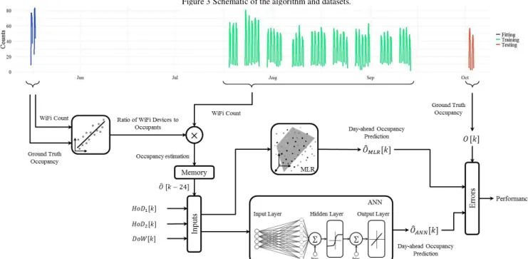
As shown in Figure 2, three WiFi sensors are placed at each floor of the studied building to ensure that the entire occupied area in the building is covered. Furthermore, in order to collect the ground truth occupancy data, the three building entrances (two on the first floor and one on the second floor) were manually monitored by volunteer employees for the duration of the test. This practice resulted in high-accuracy ground truth data aggregated at 15-minute time intervals. However, due to the cost involved with engaging manual labour, the ground truth data collection had to be limited to only two days within the working hours, which was between 7:00 AM and 5:00 PM on the first day and between 7:30 AM and 4:30 PM on the second day. In total, we obtained 78 instances of ground truth data that were used for fitting the occupancy to WiFi data, which is to identify the parameters of the model shown in Equation (2). Furthermore, the collected WiFi data is truncated to match the daily schedule of the building employees and availability of ground truth data. This implies that only data within the time span of 7 AM to 5 PM is kept and the rest is discarded. In fact, this is a more conservative approach for the sake of model accuracy. If the after-hour data (corresponding to night time and weekend hours) was kept, the model would simply predict zero occupancy during those on-occupied hours and it would create a misleading interpretation of high precision [12]. A summary of the algorithm including the available datasets is shown in Figure 3. The data collection process at the studied building consists of three time-separated tests carried out between May 2018 and October 2018. In the first test, fitting data (blue lines in Figure 3) consisting of WiFi device counts and ground truth occupancy data were

collected, with the purpose of identifying the ratio of WiFi devices to occupants. In the second extended test, WiFi counts (green lines in Figure 3) were collected but no ground truth data was available. This set of data is used to train and validate the two prediction methods based on MLR and ANN models. Finally, a third test was carried out by collecting both WiFi counts and ground truth data during two days of normal building operation, with the aim of testing the performance of prediction models. As a result, only 10% of the dataset contains ground truth data. The results of these tests are discussed in the following sections.

B. WiFi to Occupant Ratio

In the first data collection effort, WiFi and ground truth data were collected at 15-minute intervals to identify the parameters of Equation (2). The bias is interpreted as the effect of static WiFi devices such as printers and other peripherals which transmit WiFi packets even if there are no occupants present in the building. Therefore, we identify the bias by calculating the average value of WiFi[k] during the night, when occupancy count ̂[�] is expected to be equal to

Figure 3 Schematic of the algorithm and datasets.

Figure 2 Location of sensors and manual counting (at the entrances) for the three floors of the studied building.

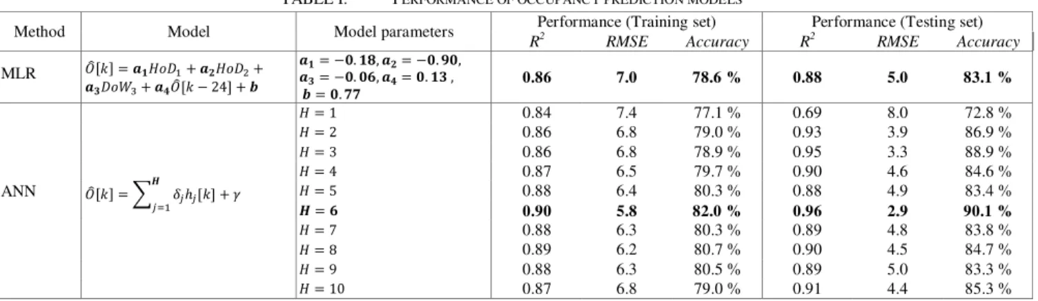
TABLE I. PERFORMANCE OF OCCUPANCY PREDICTION MODELS

Method Model Model parameters Performance (Training set) Performance (Testing set)

R2 _{RMSE Accuracy R}2 _{RMSE Accuracy}

MLR ̂[�] = �� + �� + � + ̂[� − ] + = − . , = − . , = − . , = . , = . 0.86 7.0 78.6 % 0.88 5.0 83.1 % ANN _{̂[�] = ∑}� _{ℎ [�]} = + � = 0.84 7.4 77.1 % 0.69 8.0 72.8 % � = 0.86 6.8 79.0 % 0.93 3.9 86.9 % � = 0.86 6.8 78.9 % 0.95 3.3 88.9 % � = 0.87 6.5 79.7 % 0.90 4.6 84.6 % � = 0.88 6.4 80.3 % 0.88 4.9 83.4 % � = 0.90 5.8 82.0 % 0.96 2.9 90.1 % � = 0.88 6.3 80.3 % 0.89 4.8 83.8 % � = 0.89 6.2 80.7 % 0.90 4.5 84.7 % � = 0.88 6.3 80.5 % 0.89 5.0 83.3 % � = 0.87 6.8 79.0 % 0.91 4.4 85.3 %

zero. For the studied building, the bias is equal to 27. One the bias is calculated, it is subtracted from the WiFi device count data. The resulted unbiased WiFi count is used together with the ground truth data to identify the ratio of WiFi devices to occupants. As shown in Figure 4, a linear least-squares model was fitted to 78 pairs of measurement to identify the ratio of WiFi devices to occupants, _� . The model fits the data with R2 0.9 and identifies _� to be 1.27. This implies that in average 1.27 WiFi devices are associated with each occupant in the building. It is worth mentioning that the linear fit shows an over-average correlation between WiFi device counts and ground truth occupancy in the studied building, based on a comparison to a similar linear model in [10] with R2 0.7.

C. Occupancy prediction

Supervised prediction models required a relatively large training dataset to avoid overfitting. This is especially important for more complex models such as ANN where a higher number of internal model parameters need to be identified. In this study, ground truth occupancy data serve as labels for the supervised training, hence scarcity of such data creates a challenge. As a solution to this problem, we propose a semi-supervised training approach using an estimation of occupancy count (calculated using the linear model developed in the previous step) instead of the ground truth occupancy. As seen in Figure 3, several weeks of WiFi device counts collected at the building during working hours are used for creating the training set. These WiFi counts are multiplied by the WiFi-to-occupant ratio _� , creating a

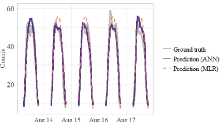
times series of estimated occupancy as an input for training the prediction models. The testing dataset, however, is comprised of both WiFi and ground truth data that were collected during the third test (depicted as red lines in Figure 3). This setup facilitates the training process of the prediction model by avoiding over training, with the compromise of reducing the accuracy of predictions as a result of not exposing the model to ground truth data. Therefore, to ensure that final performance comparisons are credible, we compare the models based on errors calculated with the ground truth occupancy data from the testing set. Table I shows the performance of occupancy prediction models for both training and testing sets as well as the corresponding model parameters. For the classic deterministic MLR model used in this study, only a single set of parameters can minimize the objective function (in this case being the least squares). Therefore, the parameters of the MLR model cannot be adjusted. On the contrary, ANN might be created in various architectures characterized by the number of hidden layer neurons. We examined the performance of ANN models as a function of the number of hidden neurons, H, as defined in equation (5). The results suggest that the best performance metrics are obtained with the ANN model when � = , achieving an accuracy of 82% for the training set (using estimated occupancy) and 90% for the testing set (using ground truth occupancy). Furthermore, almost all ANN models perform better than the MLR model, implying that the ANN is successful in capturing nonlinear relationships between the input set and the occupancy count. That being said, even the MLR model has a promising performance when compared to similar studies. For example, the best prediction models in [13] achieved accuracies of less than 50% for a horizon of 10 time steps (compare to 24 time steps in our case). One explanation is that office buildings show a more regular occupancy pattern compared to institutional buildings (such as universities). Another reason might be the relatively short length of training and testing sets in this study, as both R2 and RMSE are sensitive to the length of data. A visual comparison of the predictions based on the training dataset achieved with MLR model and the best-performing ANN model is shown in Figure 5 for five weekdays in August 2018. The difference in predictions is negligible, as both models are able to capture the hourly dynamics of the occupancy very well. However, it is observed that the MLR predictions are rather uniform among the days, implying that the dominant predictors are the

temporal features. The same conclusion can be made by comparing the value of the weight (corresponding to ̂[� − ]) with values of and (corresponding to HoD inputs). On the contrary, the ANN predictions are more correlated with the values on the day before, showing the capability of ANN model in following changes in the occupancy pattern. For the same reason, the ANN model achieves an advantage of 1.2 (5.8 versus 7.0) in RMSE. While the performance of presented prediction models is acceptable, higher accuracies might be required for certain applications. In that case, it is recommended that the more recent historical values (such as 1 hour before) are chosen as input to the prediction models. A downside to this approach is the requirement for the prediction model to be called at every hour, which might not always be feasible.

IV. CONCLUSIONS

In this paper, methods for real-time estimation and day-ahead prediction of total building occupancy count were presented. The ratio of WiFi devices to occupants in the building was identified with a linear regression model. This ratio is a characteristic of the building and its occupants and is assumed to be time-invariant for the duration of our tests. Two different prediction models based on multiple linear regressions and artificial neural networks were calibrated with an estimation of occupancy counts. The day-ahead prediction results suggested that ANN has superiority with regard to accuracy, although MLR showed competitive performance making it a better solution for situations where implementation of ANN is computationally not feasible, or in case the model intuitiveness is important to the building operators. A key advantage of the proposed approach is its limited dependency on availability of ground truth occupancy data that might prove to be challenging or costly to collect according to the building type and tenants. Furthermore, the use of WiFi device counts as a proxy for building occupancy counts makes the method widely applicable since most commercial buildings today are equipped with a WiFi network. However, there are certain limitations to the proposed method. For example, if the access points cannot be interfaced to obtain the list of MAC addresses, dedicated WiFi sensors are needed instead, which will add to the capital costs of the project. Also, in case the security policy of the building does not allow the collection of un-encrypted MAC addresses, it will be impossible to remove redundant

addresses form the populated list. It is expected that such a scenario would dramatically reduce prediction accuracy.

For future work, the authors intend to apply the proposed prediction method to data from other buildings with different utilisation types. This would allow us to compare the value of

� for each building as well as identifying the longest

period of time for which the ratio can be considered as constant. Also, there will be a focus on alternative prediction targets, such as peak daily occupancy, as well as the earliest arrival and latest departure of occupants.

ACKNOWLEDGMENT

The authors would like to thank Ron Hu, technical officer at NRC Canada, for his contributions to this study.

REFERENCES

[1] T. Hong and H.-W. Lin, “Occupant behavior: impact on energy use of private offices,” 2013.

[2] F. Oldewurtel, D. Sturzenegger, and M. Morari, “Importance of occupancy information for building climate control,” Appl.

Energy, vol. 101, pp. 521–532, 2013.

[3] X. Zhou, D. Yan, and G. Deng, “Influence of occupant behavior on the efficiency of a district cooling system,” in IBPSA

Conference, 2013.

[4] J. Yang, M. Santamouris, and S. E. Lee, “Review of occupancy sensing systems and occupancy modeling methodologies for the application in institutional buildings,” Energy Build., vol. 121, pp. 344–349, 2016.

[5] R. Melfi, B. Rosenblum, B. Nordman, and K. Christensen, “Measuring building occupancy using existing network infrastructure,” in Green Computing Conference, 2011, pp. 1–8. [6] W. Shen, G. Newsham, and B. Gunay, “Leveraging existing

occupancy-related data for optimal control of commercial office buildings: A review,” Adv. Eng. Informatics, pp. 230–242, 2017. [7] H. B. Gunay, A. Ashouri, W. Shen, G. R. Newsham, and W.

O’Brien, “A preliminary analysis on the use of low-cost data streams for occupancy count estimation,” ASHRAE Trans., 2019. [8] B. Balaji, J. Xu, A. Nwokafor, R. Gupta, and Y. Agarwal,

“Sentinel: occupancy based HVAC actuation using existing WiFi infrastructure within commercial buildings,” in ACM Conference

on Embedded Networked Sensor Systems, 2013, p. 17.

[9] B. W. Hobson, D. Lowcay, H. B. Gunay, A. Ashouri, and G. R. Newsham, “Opportunistic occupancy-count estimation using sensor fusion: A case study,” Build. Environ., vol. 159, 2019. [10] M. M. Ouf, M. H. Issa, A. Azzouz, and A.-M. Sadick,

“Effectiveness of using WiFi technologies to detect and predict building occupancy,” Sustain. Build., vol. 2, pp. 1–10, 2017. [11] S. Petersen, T. H. Pedersen, K. U. Nielsen, and M. D. Knudsen,

“Establishing an image-based ground truth for validation of sensor data-based room occupancy detection,” Energy Build., vol. 130, pp. 787–793, 2016.

[12] H. Zou, H. Jiang, J. Yang, L. Xie, and C. Spanos, “Non-intrusive occupancy sensing in commercial buildings,” Energy Build., vol. 154, pp. 633–643, 2017.

[13] J. Howard and W. Hoff, “Forecasting building occupancy using sensor network data,” in International Workshop on Big Data,

Streams and Heterogeneous Source Mining, 2013, pp. 87–94.

[14] F. C. Sangogboye and M. B. Kjærgaard, “PreCount: a predictive model for correcting real-time occupancy count data,” Energy

Informatics, vol. 1, no. 1, p. 12, 2018.

[15] E. Vattapparamban, B. S. Çiftler, I. Güvenç, K. Akkaya, and A. Kadri, “Indoor occupancy tracking in smart buildings using passive sniffing of probe requests,” in 2016 IEEE ICC

Conference, 2016, pp. 38–44.

[16] J. Martin et al., “A study of MAC address randomization in mobile devices and when it fails,” Proc. Priv. Enhancing

Technol., vol. 2017, no. 4, pp. 365–383, 2017.

[17] I. London, “Encoding cyclical continuous features,” 2016. [Online]. Available: https://ianlondon.github.io/blog/encoding-cyclical-features-24hour-time/.