HAL Id: hal-02394498
https://hal.archives-ouvertes.fr/hal-02394498
Submitted on 4 Dec 2019
HAL is a multi-disciplinary open access archive for the deposit and dissemination of sci-entific research documents, whether they are pub-lished or not. The documents may come from teaching and research institutions in France or abroad, or from public or private research centers.
L’archive ouverte pluridisciplinaire HAL, est destinée au dépôt et à la diffusion de documents scientifiques de niveau recherche, publiés ou non, émanant des établissements d’enseignement et de recherche français ou étrangers, des laboratoires publics ou privés.
Computer-aided neurophysiology and imaging with
open-source PhysImage
John Hayes, X Papagiakoumou, Pierre-Louis Ruffault, Valentina Emiliani,
Gilles Fortin
To cite this version:
John Hayes, X Papagiakoumou, Pierre-Louis Ruffault, Valentina Emiliani, Gilles Fortin. Computer-aided neurophysiology and imaging with open-source PhysImage. Journal of Neurophysiology, Amer-ican Physiological Society, 2018, 120, pp.23 - 36. �10.1152/jn.00048.2017�. �hal-02394498�
INNOVATIVE METHODOLOGY
Neural Circuits
Computer-aided neurophysiology and imaging with open-source PhysImage
XJohn A. Hayes,1 XEirini Papagiakoumou,2,3 XPierre-Louis Ruffault,1 Valentina Emiliani,2 and XGilles Fortin1
1UMR9197, CNRS/Université Paris-Sud, Institut des Neurosciences Paris-Saclay, Université Paris-Saclay, Gif-sur Yvette,
France;2UMR8250, Neurophotonics Laboratory, CNRS, Paris Descartes University, Paris, France; and3Institut National de
la Santé et la Recherche Médicale-Inserm
Submitted 24 January 2017; accepted in final form 22 February 2018
Hayes JA, Papagiakoumou E, Ruffault PL, Emiliani V, Fortin G. Computer-aided neurophysiology and imaging with open-source PhysImage. J Neurophysiol 120: 23–36, 2018. First published Febru-ary 28, 2018; doi:10.1152/jn.00048.2017.—Improved integration be-tween imaging and electrophysiological data has become increasingly critical for rapid interpretation and intervention as approaches have advanced in recent years. Here, we present PhysImage, a fork of the popular public-domain ImageJ that provides a platform for working with these disparate sources of data, and we illustrate its utility using in vitro preparations from murine embryonic and neonatal tissue. PhysImage expands ImageJ’s core features beyond an imaging pro-gram by facilitating integration, analyses, and display of 2D wave-form data, among other new features. Together, with the Micro-Manager plugin for image acquisition, PhysImage substantially im-proves on closed-source or blended approaches to analyses and interpretation, and it furthermore aids post hoc automated analysis of physiological data when needed as we demonstrate here. Developing a high-throughput approach to neurophysiological analyses has been a major challenge for neurophysiology as a whole despite data analytics methods advancing rapidly in other areas of neuroscience, biology, and especially genomics.
NEW & NOTEWORTHY High-throughput analyses of both
con-current electrophysiological and imaging recordings has been a major challenge in neurophysiology. We submit an open-source solution that may be able to alleviate, or at least reduce, many of these concerns by providing an institutionally proven mechanism (i.e., ImageJ) with the added benefits of open-source Python scripting of PhysImage data that eases the workmanship of 2D trace data, which includes electrophys-iological data. Together, with the ability to autogenerate prototypical figures shows this technology is a noteworthy advance.
calcium imaging; holographic optogenetic stimulation; image analy-ses; whole-cell patch-clamp
INTRODUCTION
To solve neurophysiological problems increasingly requires investigators to merge technical approaches such as
electro-physiological recordings, live-cell imaging like voltage/Ca2⫹
imaging (Grienberger and Konnerth 2012; Peterka et al. 2011), and optogenetic stimulation/inhibition (Boyden et al. 2005; Emiliani et al. 2015; Li et al. 2005; Lima and Miesenböck 2005). An array of different software and hardware is typically required
for researchers to meaningfully integrate these data. To simplify this type of workflow, we have developed PhysImage, a tool that builds upon the widespread utility of Micro-Manager (Edelstein et al. 2010) and ImageJ (Schneider et al. 2012) and is an all-in-one open-source software platform for acquiring imaging and physi-ology data, analyzing and processing data, and finally presenting rapid results in the form of processed figures potentially suitable for publication, or at least suitable for prototype reports. Finally, the platform can be used for integrating the logical execution of certain hardware and software analyses during the course of experiments. These functions enable the development of increas-ingly sophisticated experimental protocols in neurophysiology.
Here, we illustrate these principles using several examples in the context of systems neuroscience using murine tissue in vitro. First, we present a scripting mechanism for controlling image-related analysis operations that tie together the generation and/or manipulation of imaging and waveform data. After that, we show how to import electrophysiology data from Axon Binary Files (ABFs) recorded in pClamp (Molecular Devices, Sunnyvale, CA) and perform several types of analyses on these waveform data. We then transition into analyzing live calcium imaging data, working with their time series records, and performing some similar analysis with concurrent electrophysiology recordings and automated figure generation. Building on these examples we show how similar approaches can be used for automatable high-throughput analyses of imaging/electrophysiology data. Finally, we conclude by showing how we have integrated these ap-proaches to perform optogenetic experiments. These use comput-er-generated holographic laser stimulation (Kam et al. 2013) of variable subsets of neurons identified using calcium activity while monitoring population activity through nerve recordings.
A significant effort was made to ensure most of these examples and figures are generated with scripts for reproducible and trans-parent results (Ioannidis 2005), and serve as pedagogical exam-ples. These scripts are included with the main distribution of
PhysImage in the “Plugins¡Paper_Examples” menu tree, with
the most pertinent coding points discussed in the Results section below and much of the raw data needed to generate the example analyses are here: https://osf.io/qf2d3/.
MATERIALS AND METHODS
Software. Public-domain ImageJ software (https://imagej.nih.gov/) as well as open-source JFreeChart (http://www.jfree.org/jfreechart/), Jython (http://www.jython.org/), and VectorGraphics (http://trac. Address for reprint requests and other correspondence: J. A. Hayes,
Depart-ment of Applied Science, ISC 3, The College of William and Mary, Williams-burg, VA 23185 (e-mail: [email protected]).
erichseifert.de/vectorgraphics2d/) were integrated to form the initial foundation of the newly implemented PhysImage code we produced (http://physimage.sourceforge.net/). The integrated suite of software may be downloaded from here: https://sourceforge.net/projects/ physimage/files/latest/download. Installation instructions may be found here: http://physimage.sourceforge.net/installation/installa-tion.html. Java class objects and packages used by PhysImage are distinguished within the text using monospaced font and method names are indicated as follows: class_name::method_name() and the structure illustrated in Fig. 1.
Mice and preparations. Animal experiments were done in accor-dance with the guidelines issued by the European Community and have been approved by the research ethics committees in charge (Comités d’éthique pour l’expérimentation animale) and the French
Ministry of Research. Ca2⫹-imaging and electrophysiology in vitro
experiments were performed as described previously for pre-Bötz-inger complex (preBötC) slices (Thoby-Brisson et al. 2005) as well as for experiments using isolated embryonic hindbrains (Ruffault et al. 2015; Thoby-Brisson et al. 2009).
Imaging and electrophysiology. Briefly, for functional Ca2⫹ -imag-ing, a cooled Neo sCMOS camera (Andor Technology, Belfast, UK) was used in Global Exposure mode on an Eclipse FN1 microscope (Nikon Instruments, Tokyo, Japan). A “Frame_out” transistor–tran-sistor logic voltage signal, marking the time each frame was acquired, was routinely recorded directly from the camera through the Digidata 1550 A/D device with pClamp10 software (Molecular Devices) to allow alignment of imaging and electrophysiology recordings. A
Nikon⫻40 objective was used for Figs. 5, 8, and 9 [NA 0.80 and
working distance (WD) 2.0], while a Nikon⫻4 objective was used for
Fig. 6 (NA 0.13 and WD 17.1). Patch recordings (Fig. 4) were performed using a Multiclamp 700B using the aforementioned pClamp10. Field (Fig. 3) and nerve (Figs. 6 and 9) recordings used a Grass 7P511 high-gain AC amplifier (Grass Technologies, Warwick, RI) with Neurolog integration (Digitimer, Hertfordshire, UK).
“Online” analysis of Ca2⫹-imaging data was performed using a
PhysImage module controlling an optional LabJack U3 device (Lab-Jack, Lakewood, CO) through a 10 V digital-to-analog converter (LJTick-DAC, LabJack). A Micro-Manager Beanshell script (http:// www.beanshell.org/) acquires time series images and calculates the ⌬F/F and sends an analog voltage signal to the Digidata in real-time along with simultaneous electrophysiological (i.e., nerve) recordings.
“Offline” analysis of Ca2⫹-imaging data were performed after
acqui-sition on the image time series using ⌬F/F processing PhysImage
plugins described in the text.
Holographic stimulation. Holographic patterned optogenetic stim-ulation of ChR2-expressing parafacial respiratory oscillator (epF) neurons (Ruffault et al. 2015) was performed with an optical system built as described in detail elsewhere (Yang et al. 2011; Zahid et al. 2010), using a 300-mW maximum power diode-pumped solid-state laser emitting at 473 nm (CNI, MBL-FN-473) and custom software to control the spatial light modulator (LCOS-SLM) device (Hamamatsu, X10468-01). The laser beam, after being expanded and spatially
filtered, illuminated the active area of the LCOS-SLM (16⫻12 mm),
which was then imaged at the back focal plane of the objective by a telescope of lenses such as to fill its back aperture (see Zahid et al. 2010 for further details). Phase modulation created a laser pattern at the sample plane simultaneously illuminating multiple regions of interest (ROIs). The custom software (Lutz et al. 2008) received input from PhysImage to generate the appropriate holographic phase masks
for creating the photostimulation patterns, as described underRESULTS.
The laser pulses were generated using a PhysImage plugin that drove the same LabJack U3 device, as above, with its 10 V DAC to activate the laser’s analog input at random intervals and customizable intensities. ij gui io macro measure plugin filter frame tool process text wave plugins ChartPlugIn.java Analysis_General_Tools Analysis_ROI_Tools Analysis_Wave_Tools Automated_Acquisitions CTA_ROI_Tools CTA_Wave_Tools EPSC_Analyses Export_ROI_Tools Export_Wave_Tools Filters Hardware Hardware_Holographic Paper_Examples Processing_Tools Programming Protocols Visualization_Tools_ROIs Visualization_Tools_Waves
org physimage ephys abf
edf
PhysImage
Expansion
Modules
ImageJ1
Core
Modules
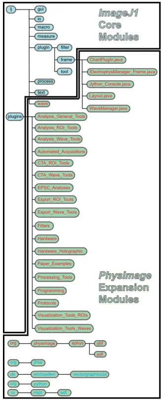
ElectrophysManager_Frame.java Jython_Console.java Layout.java WaveManager.java jfree de erichseifert vectorgraphics2d python org ru mipt edf orgFig. 1. Block diagram displaying the relationship between standard ImageJ software packages and the PhysImage extension modules. The module orga-nization relates to the directory tree that the source code is contained within. Generally, ImageJ packages have a cyan background with black text and PhysImage packages introduced in this project have green background. Open-source packages that are used by PhysImage have blue text and a green background, and newly written software, by the authors, has red text and a green background. Files ending in .java, reflect the specific class objects described in the main text (such as ChartPlugIn, Jython_Console, etc.) and reflect the location of these code in the directory tree.
RESULTS
Python control of ImageJ/Micro-Manager through Jython integration. To integrate raw imaging data, analyzed imaging
data, and electrophysiology data, we forked the Java program-ming code of ImageJ (Schneider et al. 2012). This was neces-sary to provide a platform for merging these disparate data together in a reproducible way. Toward that goal, we embedded the high-level programming language, Python, into the ImageJ interface using Jython (Juneau et al. 2010), an open-source Java implementation of Python. A high-level block diagram of pack-ages that outline the standard ImageJ software and how they relate to the extension modules included in PhysImage package are displayed in Fig. 1. New modules and key class objects that were produced by us are in red text with green backgrounds. The core Jython library appears as org.python in Fig. 1. Figure 2A illustrates the Jython console that appears in
PhysImage (ij.plugin.frame.Jython_Console.java
in Fig. 1). Because of Jython’s ability to control Java code, combined with the relative simplicity of Python syntax and coding, the console coordinates the flow of data sources and analyses. It does this by allowing us to utilize ImageJ plugins,
such as Micro-Manager (Edelstein et al. 2010), as well as ImageJ macros, or new and novel functionality that can arise from custom code taking advantage of Jython’s ability to mix Java and Python code cooperatively and nearly seamlessly.
Standard ImageJ already has support for writing and record-ing its own simple macro language for later playback. There is support for additional scripting languages as well such as Python, Ruby, and Javascript, among others. However a key difference here is that PhysImage always records interactions with the program interface in the background. The code for most actions is written to the console so that anyone can copy and paste them into scripts for later execution. For example, if the user opens an image file through the File¡Open dialog and then runs Process¡Filters¡Gaussian Blur..., something like the following will be reported on the console:
openImage(“/Users/default/Example1.tif”);
run(“Gaussian Blur...”, “sigma⫽1”);
This can be copied and pasted directly into a script or console for reuse later, and actions like these can be mixed with more conventional Python programming logic in the
B
A
B
a
clears the console history
b
save/load .py codec
copy/paste to and from the system’s clipboard
C
Fig2C.py
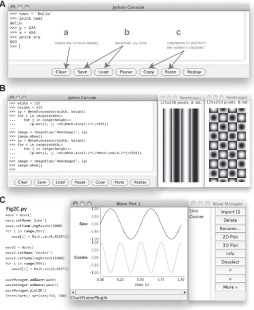
Fig. 2. Programmatically manipulating the PhysImage environment. A: the central Python console integrated into the PhysImage interface. B: Python code (left) that is described in the main text and generates 2 images (middle and right). C: Python code (left) that generates sine and cosine Waves. Middle: plots of the sine and cosine Waves. Right: the WaveManager win-dow is used to collect and manipulate Waves.
console or scripts, which provides for rapid prototyping of trivial and even nontrivial scripts.
A significant benefit of embedding the interactive console in the program is that it immediately interprets and executes any code typed. For example, typing the following code into the console will result in output that looks like Fig. 2A:
text ⫽ ‘Hello’
print text
The rest of Fig. 2A demonstrates some other code that assigns values to variables and performs simple arithmetic.
Figure 2B is a more elaborate example illustrating how the console may be used to access the ImageJ application program-ming interface (API) to manipulate images. In this example, two simple images are dynamically generated by incrementally looping over the coordinates of the images and performing a trivial trigonometric calculation to set the pixel intensities of the images. ImagePlus and ByteProcessor are special classes of objects provided by the ImageJ API, which itself is superseded by the more expansive PhysImage API (http:// physimage.sourceforge.net/physimage_api/index.html). Math, in turn, is a class within the standard Java library that provides implementations for the sin and cos functions (https://docs. oracle.com/javase/8/docs/api/java/lang/Math.html). Finally,
range is a special built-in function of Python (https://docs.
python.org/2/library/functions.html) that offers a succinct way to loop over a range of numbers. In pseudo-code the Python in Fig. 2B could be described as follows:
·assign 125 and 250 to the “width” and “height” variables, respectively
·create a ByteProcessor that stores the pixel values for the first image
·loop over the columns of the image (i.e., from 0 to 124)
·loop over the rows of the image (i.e., from 0 to 249)
·set the value of pixel (i,j) to
sin(0.1*i)*256
·generate and show the ImagePlus object to display the ByteProcessor
·generate another image with a different calculation for the pixels
Code like the above may be saved into a text file with a .py file extension and run as an ImageJ plugin. The chief criterion to accomplish that is the file must be saved in the “plugins” directory tree, as other ImageJ plugins, and an entry for it will appear in a Plugins submenu after restarting PhysImage. If
jEdit is installed (http://jedit.org), one can just click the
plugin-name in the submenu while holding Ctrl down to open the script code to edit it after it has been loaded into your menu, save it, and the changes will be reflected the next time the .py plugin is run without restarting PhysImage.
A final benefit of embedding the Jython interpreter is that its execution has access to core ImageJ code that is otherwise hidden from the user. As a consequence, it provides a means of persistence across plugins and scripts that is not otherwise present or easily accessible from ImageJ plugins. For example,
PhysImage relies on a large number of parameters whose
values are stored in a Configuration_ class object and persists across plugins and scripts. In particular, a “base direc-tory” is frequently used in both analysis and acquisition scripts as seen in subsequent subsections. All these values can be
programmatically manipulated and the most commonly changed values may be changed from the “Plugins¡Analysis_General_ Tools¡Analysis_Configuration” dialog.
Together, these features allow rapid prototyping of a se-quence of actions, by a combination of graphical interaction and coding interactivity, to create sophisticated scripts for later playback. To illustrate this quality, most of the figures in this manuscript have corresponding scripts with the main
Phys-Image distribution that demonstrate how to generate them from
sample raw data. The following sections illustrate how the expanded features of PhysImage can be used to work with physiological data acquired under various conditions.
Chart generation of time series data. The analysis of
imag-ing data are ImageJ’s principal forte, but time series data need to frequently be acquired and analyzed to solve physiological questions as well (these time series may be derived from uniformly sampled time series or elsewhere). To strengthen
ImageJ’s ability to manipulate time series data, we have added
the ability to manipulate one-dimensional waveforms, or “Waves,” similar to images within ImageJ.
Waves can be generated programmatically, by importing the data from other software files, pasted from ASCII text at the system clipboard, or imported from imaging time series ROIs.
Waves may be displayed with ChartPlugins (ij.
plugin.frame.ChartPluginin Fig. 1), which can
dis-play many types of time series data. ChartPlugIns provide convenience functions for making some simple changes to the format of the graphics. This was implemented by incorporating the open-source JFreeChart package (Gilbert 2002; org.
jfreein Fig. 1), which provides an extensive library of chart
functionality that may be programmatically accessible from the ChartPlugIns when convenience functions are not already available for maximum flexibility.
Waves may be collected into the WaveManager, analo-gous to ImageJ’s RoiManager. This provides an easy way to manipulate several Waves and perform such operations as copying/saving the contents, normalizing and scaling the val-ues of the Waves, or reordering/renaming the Waves. The
WaveManageris also a useful place to store waves and may
be programmatically added or removed and offers the flexibil-ity to transform the 1D data from the scripting environment like in MATLAB (MathWorks, Natick, MA) or other mathe-matical software tools. With access to the waveform data, the contents may be manipulated with fine granularity and may be used in many PhysImage plugins. Finally, multiple Waves can be selected and plotted or analyzed with other plugins.
To illustrate these concepts, Fig. 2C shows how to dynam-ically generate two waves that represent sine and cosine wave-forms in two dimensions. The code is similar to Fig. 2B in that it uses the Java Math class for sin/cos functionality and the Python range function for looping. However, this code as-signs the sin/cos values to specific indices of the Wave arrays instead of image pixel locations and then adds the Waves to the WaveManager to plot them using a ChartPlugIn with the plot2D() function. The plot2D() itself is just a convenience function for calling the “Visualization_Tools_Waves¡Wave_ 2DPlot” plugin from the PhysImage menus, while calling the latter directly provides more options for displaying the selected wave(s) in the WaveManager. There is also a plot2D() convenience function that can be called directly from a Wave reference like so:
wave1.plot2D()
or from the Waves class that can be used for collecting a set of Waves. For example,
waves ⫽ Waves()
waves.addWave(wave1) waves.addWave(wave2) waves.plot2D()
is equivalent in outcome to the previously illustrated code that uses the WaveManager. The key difference is that the
WaveManager provides a graphical window that is
some-times more convenient for manipulating the Waves than pro-grammatically working with them. Most of the other Wave-related plugins packaged with PhysImage start with assuming that the Waves to be manipulated are in the WaveManager. By default, Waves represent time series waveforms so the abscissa of the resulting plots are in seconds and the scale is determined by the sampling rate specified by the value passed to the Wave::setSamplingRateHz() function. Later exam-ples show additional ways of displaying the contents of Waves.
Importing electrophysiological data. Although generating
Waves from scratch can be useful, the principal utility of Waves is derived from storing and manipulating experimental data with them. One type of experimental data that may be imported as Waves come from analog-to-digital converter
(ADC) devices saved in electrophysiological files (“ephys files”). Within PhysImage, these files are internally saved as
EphysFileobjects specified in the
org.physimage.ep-hyspackage (Fig. 1) and agnostic to the underlying source of
electrophysiological file. For our examples in this paper, we used an Axon Instrument’s Digidata ADC, along with their
pClamp10 software, to record our electrophysiology data in
many different channels and save the data, metadata, and related comments into ABF format (ABF/.abf files). We have added the ability to read ABF files directly within PhysImage where data may be imported into the WaveManager by developing an ABF class object (specified in org.physimage.ephys.abf, Fig. 1) that extends the EphysFile interface. However, other elec-trophysiology storage file formats can easily be supported as well,
such as the openly specified European Data Format (EDF⫹,
http://www.edfplus.info/) that is commonly used for EEG/EMG/ ECG data. We have added a respective EDF class object (specified in org.physimage.ephys.edf, Fig. 1) that functions sim-ilar to ABF as an extended EphysFile and can read .edf files. We have also introduced an ElectrophysManager (Ephys_ Manager, Fig. 3A) that dynamically detects new ephys files, irrespective of their underlying source whether .abf, .edf., etc., or any other extended EphysFile, in the currently defined base directory and reports any new files when the window is opened. It
A
ephys files in the base directory (3) comments across all ephys files (2) easily switch base directory (1) enter a name for an epoch to import into WaveManager an epoch is defined as a regionwithin the ephys file corresponding to some event of interest. For example, an imaging epoch that may correspond to a time-series acquisition (the above was roughly 1 min).
(5)
Clear the cache to update the ephys files' metadata
(4)
B
D
B
0.00 25.00 50.00 75.00 100.00 125.00 150.00 175.00 200.00 225.00 250.00 275.00 300.00 325.00 350.00 375.00 time (s) 0.45 0.50 0.55 0.60 0.65 pbcC
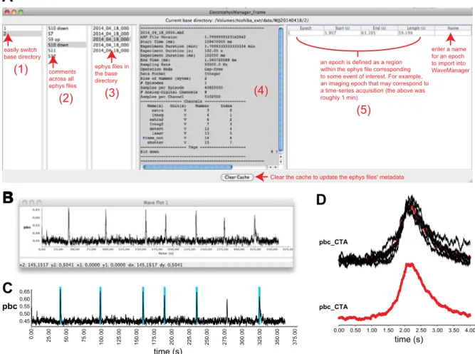
pbc_CTA 0.00 0.50 1.00 1.50 2.00 2.50 3.00 3.50 4.00 time (s) pbc_CTAFig. 3. Loading and manipulating electrophysiology data in PhysImage. A: the ElectrophysManager window may be used to navigate across experiments, view metadata including tags/comments, detect epochs of data, and import channel data into the WaveManager. B: a field recording of a medullary slice retaining the respiratory rhythm generator. C: the same field recording showing detected bursts annotated using vertical bars exported as an EPS file. D: a cycle-triggered average window (bold) of bursts identified in C and displayed in the lighter shades with a red mean in the bottom trace. pbc, Integrated pre-Bötzinger complex activity; pbc_CTA, cycle-triggered averages of these data.
provides a means to interactively view summary information associated with each file and contains metadata such as the number and names of channels recorded, the length of the file, associated tags/comments, sampling rate, etc. The middle panel principally shows this metadata while the left three panels main-tain lists that can be used to navigate through the data easily.
The panel just to the left of the metadata panel shows the list of ephys files in the base directory. The middle-left panel shows a list of comments (“tags” in pClamp parlance) across all the ephys files in the base directory. New comments may be inserted and other comments edited or deleted, and selecting a comment will also select and retrieve the ephys file the tag was associated with. The far left panel shows other directories that are siblings of the current base directory. Selecting a different sibling will change the current base directory and reload the ephys files, which makes it easier to navigate across experiments.
The entire channel contents of a selected ephys file may be imported into the WaveManager, or just a subsection of the file based on a user-defined window of time, i.e., an “epoch,” where the channel name will provide the associated Wave name. Epochs of data sent to the WaveManager may be defined in several ways. The first is simply based on a user-defined range of time. A second way is with a search feature built in to PhysImage that uses one of the channels of electrophysiological data to define the start and stop of an epoch such as when an image acquisition has started or stopped. In the following part, we illustrate how to import data using the first approach over a user-defined range.
Figure 3B shows an extracellular field recording from the preBötC in a transverse slice of the medulla oblongata from a newborn mouse brain, which retains the ability to generate respiratory network oscillations (Funk and Greer 2013; Smith et al. 1991). A selected ephys file was right-clicked within the ElectrophysManager and the “Send data to WaveManager” option was picked. This popped up a window giving the minimum and maximum time of the file in seconds where an intervening interval may be specified. When importing from ephys files the sampling rate, units, and tags for the interval
will be associated with the Wave and can be accessed from the “Info” button of the WaveManager, or programmatically via the WaveManager::info() function, or the
Wave::g-etInfo()function of the Wave class.
With data like these, it may be of interest to automatically identify the bursts of activity in the “preBötC” recording and average them to determine the general trajectory of the bursts. Figure 3C shows blue WaveMarkers that indicate automat-ically identified bursts that uses a “CTA From Wave and Above AbsThreshold” plugin we wrote. The “CTA” represents a cycle-triggered average whose mean is shown in red in Fig. 3D with the raw cycles in black in the top panel. Similarly, period information may be extracted using the blue
Wave-Markersillustrated in Fig. 3C.
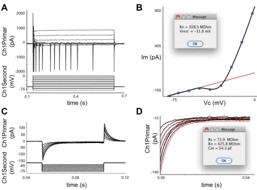
Other types of experiments stored in ephys files represent episodic protocols where a long stretch of recording is essentially the concatenation of multiple sweeps of recording. For example, current-voltage recordings from neurons are often recorded and represented in this manner (Fig. 4A). These may be imported as specialized EpisodicWaves into the WaveManager. The different class of object denotes the different way the traces will be shown in a ChartPlugIn, but it also provides expanded logical access to the underlying data to facilitate programmatic control. This can be leveraged in a few ways. First, traces may be easily queried to report the mean values at each step from 0.5 to 0.6 s like so (Fig. 4B): iwaves ⫽ WaveManager.getWave(‘Ch1Primar’) vwaves ⫽ WaveManager.getWave(‘Ch1Second’) iwave ⫽ iwaves.getMeanValues(0.5, 0.6) vwave ⫽ vwaves.getMeanValues(0.5, 0.6) iwave.setXWave(vwave) iwave.plot2D()
As in Fig. 4B, the resulting data may then be fit to report
values of physiological interest such as input resistance (RN):
lfit ⫽ LinearFitWave(iwave, 0, 2) FrontChart().addWave(lfit) rn ⫽ 1000.0/lfit.getSlope()
A
B
D
C
-50 -100 -150 -65 -75 Ch1Primar (pA) Ch1Second (mV) Ch1Primar (pA) Ch1Second (mV) time (s) 0.04 0.08 0.12 100 50 0 0 -75 0 2000 -2000 1000 -1000 0.1 0.4 0.7 time (s) time (s) 0.04 0.00 -140 -10 Vc (mV) 0 5 7 -Im (pA) -100 800 400 Ch1Primar (pA)Fig. 4. Analyses of episodic electrophysiology pro-tocols. A: a voltage-clamp step protocol showing the whole-cell membrane current recordings (top) from a medullary neuron. B: steady-state current vs. holding command voltages derived from the traces in A. The blue data points are the mean current measured between 0.5 and 0.6 s, and the black curve is a spline fit to those data points. C: brief step-protocols to determine input resistance (RN),
series resistance (RS), and membrane capacitance
(CM). D: voltage-clamp step exponential fits from
Fig. 3C detailing how to measure the whole-cell
CM, RS, and RN of a neuron. Ch1Primar and
Ch1Second, primary and secondary channel1 ac-quisitions, respectively; Im, whole-cell membrane current; Vc, command voltage.
vrest ⫽ lfit.getRoot() calcs ⫽ ‘Rn ⫽ ’ ⫹ str(format(rn, 1)) ⫹ ‘MOhm\n’ calcs ⫹⫽ ‘Vrest ⫽ ’ ⫹ str(format(vrest, 1)) ⫹ ‘mV\n’ IJ.showMessage(calcs)
EpisodicWavesalso allow logical access to the underlying
episodes so that other types of analysis may be performed. For
example, to measure the whole-cell membrane capacitance (CM),
input resistance (RN), and series resistance (RS) in voltage-clamp
configuration a step protocol like Fig. 4C may be used as we have described elsewhere (Hayes and Del Negro 2007). Then, we can
calculate the CM by integrating the difference in the current
recorded before from the current recorded during the step (IM) for
⌬Q ⫽ 兰IM. The change in charge (⌬Q) divided by the change in
command voltages (⌬Vc) during the step protocol allow us to
calculate CM(i.e., CM⫽ ⌬Q/⌬Vc). While fitting exponentials to
the charging decay allows us to calculate the RS from the time
constant (i.e., RS⫽m/CM).
Rather than just performing this calculation on one trace it is more representative to calculate it over several traces and average the results. Scripted in PhysImage, these calculations may be performed as the code for Fig. 4D with the most critical parts as follows:
rs, rn, cm ⫽ [], [], []
for iwave, vwave in zip(iwaves, vwaves):
iwave ⫽ iwave-ileak expWave ⫽ ExpFitWave(iwave) vwave ⫽ vwave-vleak rnval ⫽ iwave.getMeanValue(0.034, 0.037)/ vwave.getMeanValue() c m v a l ⫽ abs(iwave.calculateArea()/ vwave.getMeanValue()) rs.append(1e6*expWave.getTau()/cmval) rn.append(1000.0*rnval) cm.append(1000.0*cmval) calcs ⫽ ‘Rs ⫽ ’ ⫹ str(format(mean(rs), 1)) ⫹ ‘ MOhm\n’ calcs ⫹⫽ ‘Rn ⫽ ’ ⫹ str(format(mean(rn), 1)) ⫹ ‘ MOhm\n’ calcs ⫹⫽ ‘Cm ⫽ ’ ⫹ str(format(mean(cm), 1)) ⫹ ‘ pF\n’ IJ.showMessage(calcs)
In this code, iwaves and vwaves refer to the collection of current and voltage traces during the steps, iwave and vwave are a current/voltage step within the collections, and vleak and
ileakare the first voltage and current steps. ExpFitWave is an
extended Wave class that fits an exponential to raw Wave data (i.e., iwave in the above) and can be used to get the fit
charac-teristics like them. (e.g., ExpFitWave::getTau()).
Identifying neuronal activities from imaging.
Physiologi-cally relevant signals are often identified by processing raw imaging time series. A common processing step for calcium
imaging is the generation of⌬F/F traces that help discriminate
signal from noise. ⌬F/F traces are generally defined as
(F⫺F0)/F0where F0represents background fluorescence, F is
the fluorescence at a given instance, and therefore⌬F/F is the
normalized change in fluorescence. However, how the F0 is
defined can vary depending on the type and manner that a specimen is imaged. PhysImage provides several plugins that
utilize different strategies for generating time series ⌬F/F
images with the principal difference being how F0is defined.
When ROIs are plotted in 2D as a function of time from these
processed images it represents⌬F/F traces.
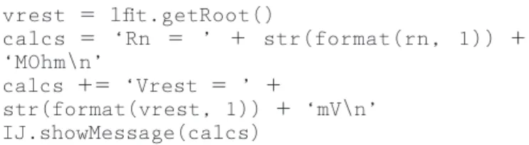
Figure 5 illustrates a time series acquisition of the epF of the murine embryo (Thoby-Brisson et al. 2009) acquired using the
Ca2⫹-indicator dye calcium green 1-AM. A frame capture
representing the raw time series is in Fig. 5A and pseudo-colored with a green lookup table. This population of neurons is characterized by periodic bursts of activity at ~0.2 Hz. A common task for scientists analyzing images with dynamically changing intensities, such as these, is to identify ROIs that
represent candidate neurons. First, the⌬F/F time series can be
generated using PhysImage’s “Forward Moving Average Fil-ter” plugin and the standard deviation of the resulting time series can be displayed (Fig. 5B). In this plugin, each frame’s
spatial pixel represents the F value in the ⌬F/F calculation,
while the F0is calculated by the mean pixel values of the next
x number of frames (100 in this case). In these data, similar to
the electrophysiological data of Fig. 3, we can produce a CTA image from bursting activity in the ROI delineated by a white outline in Fig. 5C to show which cells are on average behav-iorally related (Fig. 5D). ROIs that represent neuronal candi-dates of interest can be identified using an “ROI Detector” plugin we wrote (Fig. 5E) implementing an iterative thresh-olding algorithm (Wang et al. 2013) similar to what others have done (Mellen and Tuong 2009; Valmianski et al. 2010). Once these ROIs are identified, they can be used to generate time series plots within PhysImage. Individually, Waves can be generated by importing the data from imaging time series for each ROI (Fig. 5F, top), processed (Fig. 5F, bottom), and visualized using a 3D raster in a ChartPlugIn (Fig. 5G). ChartPlugIns can also be used to combine waves with differing sampling rates, such as electrophysiology data along with imaging data that may be sampled at a slower rate, or any arbitrary waves that may have been manually generated with a certain sampling rate.
Of note as well, is that when a Wave is retrieved from the WaveManager, the original ROI may be retrieved natively if it was produced from a time series image using Wave:: getRoi(). Spatial attributes for a Wave can therefore be easily retrieved by accessing the associated ROI. However, a
Wavecannot be produced from an ROI alone, fundamentally,
because a time series (i.e., an ImagePlus window) is essen-tial for a Wave to be produced.
Auto-generated figures using Layouts. Time series chart and
imaging data may be combined in Layouts (ij.plugin.
frame.Layout in Fig. 1), which can be used to build full
figures analogous to ones that may be printed in papers or at least serve as useful prototypes. The latter are particularly useful for stubbing out the general figure layout of analyzed data in a structured and reproducible manner across many different experiments as well as for internal reports. After a
Layout has been built, it may also be exported as
vector-based .eps files or as raster images in any format that ImageJ provides, such as JPEG, TIF, or PNG.
There are three general approaches to generating layouts. The first is to use the graphical interface and create a new Layout using the File¡New menu, which is a new addition from
Phys-Image. This creates a blank window representing a sheet of paper.
By right-clicking the field, popup menus can be used to add open charts and images to the Layout at arbitrary locations. Text
labels can be also be added in a similar manner, which is useful for annotating a report with the date or other experiment details. The second way of generating layouts is programmatically. As with many PhysImage operations, the analogous code will be represented in the Jython console in real-time as the graph-ical user interface operation commences. This makes an excel-lent starting point for creating new, more flexible, code. How-ever, the basic way to create a Layout, and add an image (e.g., here named “Image1’) and text label, is as follows:
layout ⫽ Layout()
layout.addComponent(‘Image1’, 50, 45) layout.addText(“A”, Color(0,0,0), Font(‘Arial’, Font.BOLD, 48), 15, 15)
The first line simply creates an instance of the Layout class for us to reference, the second line adds the “Image1”
compo-nent to the layout at position (x⫽ 50, y ⫽ 45) and the third line
adds a black “A” label to position (x⫽ 15, y ⫽ 15) with an
Arial, Bold font of 48 point size. Note: Color and Font are Java classes specified in the Java API documentation. Named
ChartPlugIn windows can also be added to Layouts as
“Image1” as above.
To save the layout to the computer’s file system we can use the following code:
layout.saveLayout(‘/Users/default/ Layout1.layout’) layout.exportToJpeg(‘/Users/default/ Layout1.jpg’) layout.exportToTiff(‘/Users/default/ Layout1.tif’) layout.exportToEps(‘/Users/default/ Layout1.eps’)
The first line saves the layout as a binary file that can be reproduced in PhysImage while the last three will save the layout as JPEG, TIFF, and EPS files, respectively.
The last way of generating a layout is to load charts or images into a Layout template. To make this even easier, once a layout is configured to our liking, we can save a template of that layout for later use by scripts or it can be autoloaded using any available opened images and/or charts that will be arranged according to the template.
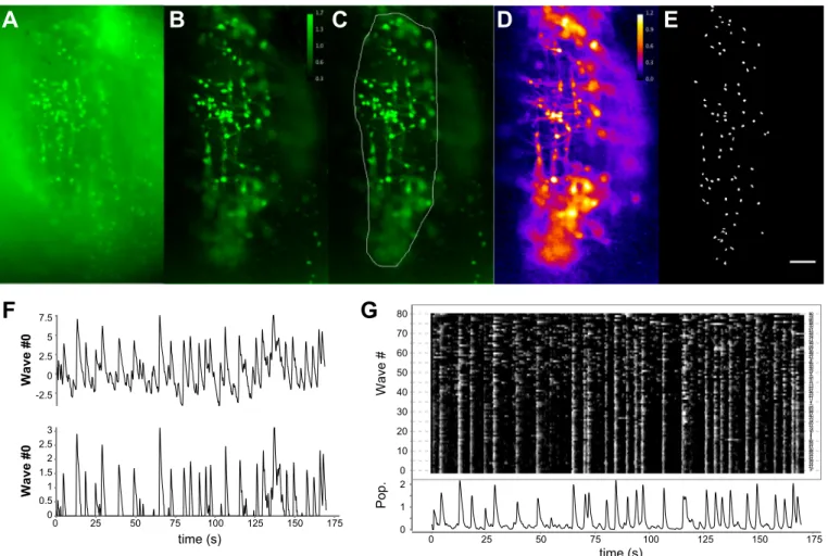
Figure 6 illustrates an example that uses the template system and many of the principles previously discussed to build each panel of the final figure. Figure 6G shows a reproduction of the
Layouttemplate used to generate Fig. 6 itself. This was
graph-ically built by adding the alphabetic labels and adding some previously opened images and chart. After that, right-clicking the
0 25 50 75 100 125 150 175 time (s) 0 10 20 30 40 50 60 70 80 Wave # 7 19 21 24 32 39 41 42 44 45 48 50 51 54 56 620569 10 14 16 31 60 74 13 20 40 57 58 63 69 7214 11 71 22 23 46 47 52 53 73 772 55 753 37 15 26 30 35 658 18 27 28 29 36 67 68 12 49 64 17 34 25 33 43 61 76 70 38 59 66 78 79 80 0 1 2 Pop.
A
B
C
D
E
G
F
-2.5 0 2.5 5 7.5 Wave #0 0 25 50 75 100 125 150 175 time (s) 0 0.5 1 1.5 2 2.5 3 Wave #0Fig. 5. Detection of neurons active during population activity by calcium imaging. A: unprocessed wide-field fluorescent imaging of calcium-loaded respiratory
neurons. B: the same field showing the maximum⌬F/F acquired over the time course. C: the same image as B with a region of interest (ROI) delineating the
region to use as reference for the imaging cycle-triggered averaging (CTA) in D. D: a CTA of the activities in the observed field. E: ROIs detected over the field
in D. The scale bar represents 50m. F, top: a single waveform derived from an ROI in E. Bottom: the same waveform processed as truncated z-scores. G, top:
a raster plot showing the Waves corresponding to the full ensemble of ROIs shown in E with analogous processing to that performed in F, bottom. Increasing
values are lighter (higher⌬F/F) and decreasing values darker (lower ⌬F/F). The ordinate positions were selected by sorting the Waves as described in the text.
layout window and the “Save layout as template...” option pro-vides a means of preserving the template on the file system.
Figure 6A shows the hindbrain with calcium imaging and a concurrent cervical nerve recording while Fig. 6B shows the
standard deviation of the CTA of⌬F/F activity. Figure 6, C and
D show identified ROIs overlaid with Fig. 6, B and A,
respec-tively. These ROIs produced the traces in Fig. 6E and the CTAs of Fig. 6F. The content of these panels may be generated with small scripts (see related content in the main distribution). Then a separate script may be used to call the smaller scripts that generate each panel with the template instantiated as follows:
Configuration_.setBaseDirectory(“data/ Fig6”) run(“Fig6a”) run(“Fig6b”) run(“Fig6c”) run(“Fig6d”) run(“Fig6e”) run(“Fig6f”) layout ⫽ Layout(“Layout_Fig6.layout. template”)
which loads the images and charts into the first slots in the template (Fig. 6G). This templating system is ideal for the col-lection stage of an experiment, where a specific protocol will be repeated many times and assist researchers to have ready access to many examples displayed the same way.
Automating experimental analyses. With this combination of
tools available, many repetitive experimental protocols and
A
G
B
C
D
E
2F
1 0 -1 0.4 0.3 0.2 0.1 3.5 3.23 1 0 1 0 -1 2.5 0 2.5 0 10 20 30 40 50 60 70 80 90 100 110 120 130 140 150 160 170 0 1 2 3 4 time (s) time (s) offline online pTRG mVlln epF vrc C4 A B C D E F GFig. 6. Combined analyses of imaging and electrophysiology data in Layouts. A: a merged view of the hindbrain-spinal cord preparation used in this figure. B:
a cycle-triggered averaging (CTA) of the⌬F/F activity in this region over 170 s. C: the same view as B with regions of interest (ROIs) outlined for respiratory
nuclei of interest. D: the same ROIs as C over the wide-field image of the hindbrain in A. The scale bar represents 200m. E: The traces of ⌬F/F in D; here
“offline” represents the cyan ROI measured after the recording, the “online” was the same region during acquisition using a LabJack (seeMETHODS), pTRG
(paratrigeminal respiratory group) are the purple ROIs, green are the embryonic parafacial respiratory group (epF) ROIs, red is facial motonucleus ROIs, and blue is the ventral respiratory column ROIs. F: the CTAs for the respective ROIs from D and E. G: The Layout template used to generate this figure.
Input S1.stk (pH 7.4) S2.stk (pH 7.2) Calc F/F Calc Stdev Calc CTA Detect ROIs Normalize detected Waves Calc F/F Calc Stdev
Detect ROIstect ROIs
Normalize detected Waves Input S1.stk (pH 7.4) S2.stk (pH 7.2) Build raster plot of activity Output Report-style Figure Calc mean activity
Fig. 7. Automated analyses of raw data across 1 or more data sets. A flowchart showing the processing pipeline of the script that produces Fig. 8. Calc, calculate; CTA, cycle-triggered averaging; Stdev, standard deviation.
analyses can now be automated. For example, Fig. 7 shows a flowchart of the analysis that produces full Layouts like Fig. 8. These Layouts are programmatically generated from raw imaging data run under different experimental conditions. This script (Fig. 8.py) uses most of the same principles that have already been presented but targeted at a more complex output for the final figure, and it notably delegates potentially redun-dant code into user-defined Python functions.
The objective of these experiments was to examine a set of mouse mutants and compare the functional viability of their epF by subjecting each to a pH challenge (Ruffault et al. 2015). The raw data were two TIFF files that respectively contain
time series calcium imaging data under pH⫽ 7.4 and
pH⫽ 7.2 conditions and whose filenames end with “.stk.”
In combination with the Programming¡Iterate_Plugin_
Through_Directory_Tree plugin the same script may be used to generate similar reports across many different sets of experiments for automated high-throughput analyses.
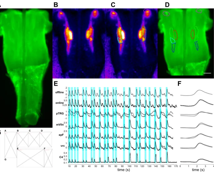
Automating experimental acquisitions and analyses. To
ex-tend these examples to acquisition and intervention during an experiment, our short-term goal was to generate a pattern of light on a relatively confined population of neurons (up to 11 in this case) and then sequentially holographically stimulate each of these targets individually (Figs. 9 and 10). To accom-plish this, we generated a .py script plugin that takes a .zip file containing the full list of target ROIs identified using an 80-s time series imaging acquisition along with online detection of
the population Ca2⫹-activity (similar to Figs. 5, 7, and 8). The
script then generates source images with target masks that are subsequently sent to the custom software controlling the SLM
Fig. 8. Autogenerated report using the analysis flowchart of Fig. 7. The top line labels the experiment directory with the raw .stk files. S1.stk from Fig. 7 represents
the calcium activity under pH⫽ 7.4 conditions while S2.stk represents the activity at pH ⫽ 7.2. The leftmost 4 images show the activity over the whole time
series (green) with autodetected regions of interest (ROIs) (red) as determined based on standard deviation (Stdev, top 2) or cycle-triggered averaging (CTA) (bottom 2). The 4 images to the right of those show the ROIs color coded so that the earliest active neurons are in warmer colors. The middle raster plots show the corresponding activities with lighter colors indicating higher activity. Note the higher number of neurons and increased coherence of activity under the
pH⫽ 7.2 conditions as compared with pH ⫽ 7.4. The far right images show overlays of the pH ⫽ 7.4 (red) and pH ⫽ 7.2 (green) conditions as determined using
the Stdev or CTA images, which highlights the new neurons activated under the pH⫽ 7.2 conditions. Pop., population.
H
G
75% laser 100% laser
Acquire Imaging/Electrophys
Identify Potential Targets
Make Target Mask
Stimulate at Random Intervals
Change Laser Intensity
Generate Analyses Reports
F
A
B
C
E
D
100% laser 0 5 10 15 20 25 30 35 40 45 50 55 60 65 70 75 80 85 90 95 100 105 110 115 120 125 130 135 0 5 10 15 20 25 30 35 40 45 50 55 60 65 70 75 80 85 90 95 100 105 110 115 120 125 130 135 0 5 10 15 20 25 30 35 40 45 50 55 60 65 70 75 80 85 90 95 100 105 110 115 120 125 130 135 0.55 0.50 0.45 0.40 0.35 0.30 0.25 0.20 0.15 0.275 0.250 0.225 0.200 0.175 0.150 0.125 0.100 0.50 0.45 0.40 0.35 0.30 0.25 0.20 0.15 Integ Integ IntegFig. 9. Optogenetic stimulation and analyses of respiratory neurons. A: a flowchart showing the analyses in both Fig. 9 and 10. B: higher magnifi-cation of the embryonic parafacial respiratory (epF)
region. C: analyzed⌬F/F of the same region as B.
D: a mask of the active neurons in C that are targets for laser stimulation. E: full population activity of the epF punctuated by random laser stimuli. The
scale bar represents 50m. F: 3 neurons stimulated
at full power (100%) repetitively. G: 10 targets in the same region stimulated with the same total laser power. H: the target from G stimulated at just 75% power and the corresponding response. Integ, inte-grate nerve activity.
device, which calculates the appropriate phase mask and proj-ects the corresponding holographic pattern for each target on the SLM. PhysImage then acquires an 80 s time series with any nerve recording while periodically generating a command pulse to our laser stimulator. The script also analyzes data from that time series similar to the previous panel and loads a
Layoutwith these data. Finally, it saves the Layout figure
to the computer’s local hard disk and then moves on to the next target until all targets have been examined. This principle is illustrated in the flowchart of Fig. 9A.
The initial set of potential targets was found over the epF as shown in Fig. 9, B–E (similar to Fig. 5). Figure 9F shows the response to stimulation at maximum power of our 473 nm laser (blue markers) on 3 autodetected ROIs (Fig. 9F, left). The
response to stimulation of 11 targets is shown in Fig. 8G with the same targets and decreased laser power in Fig. 9H.
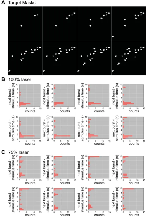
Figure 10 shows an acquired run of the full 11 targets loaded into a Layout. Following to the right and downward, the target templates are automatically loaded (Fig. 10A), the stim-ulation command is automatically set, and the figures are autogenerated to convey the distribution of laser responses relative to the spatially/temporally confined stimuli at full power (Fig. 10B) or reduced power (Fig. 10C). Notably, these data illustrate with decreased laser power that the same holo-graphic-stimulation pattern had a reduced likelihood of popu-lation entrainment by light compared with maximum power. It also shows that weak, but broad, stimulation was less effective than more potent stimulation on a restricted number of neurons
A
B
Target Masks 100% laserC
75% laser 10 8 6 4 2 0 0 5 10 15 counts next burst -stimulus time (s) 10 8 6 4 2 0 0 5 10 15 counts next burst -stimulus time (s) 10 8 6 4 2 0 0 5 10 15 counts next burst -stimulus time (s) 10 8 6 4 2 0 0 5 10 15 counts next burst -stimulus time (s) 10 8 6 4 2 0 0 5 10 15 counts next burst -stimulus time (s) 10 8 6 4 2 0 0 5 10 15 counts next burst -stimulus time (s) 10 8 6 4 2 0 0 5 10 15 counts next burst -stimulus time (s) 10 8 6 4 2 0 0 5 10 15 counts next burst -stimulus time (s) 10 8 6 4 2 0 0 5 10 15 counts next burst -stimulus time (s) 10 8 6 4 2 0 0 5 10 15 counts next burst -stimulus time (s) 10 8 6 4 2 0 0 5 10 15 counts next burst -stimulus time (s) 10 8 6 4 2 0 0 5 10 15 counts next burst -stimulus time (s) 10 8 6 4 2 0 0 5 10 15 counts next burst -stimulus time (s) 10 8 6 4 2 0 0 5 10 15 counts next burst -stimulus time (s) 10 8 6 4 2 0 0 5 10 15 counts next burst -stimulus time (s) 10 8 6 4 2 0 0 5 10 15 counts next burst -stimulus time (s)Fig. 10. Automated acquisition, analyses, holographic intervention, and an autogenerated report using PhysImage. This entire figure was produced by a PhysImage script shortly after acquisition in tandem with Fig. 9. A: images that represent the autodetected pattern of masks for holographic stimulation in B and C. The field of view encapsulates the area containing the red regions of interest in Fig. 9, D and E. B: histograms depicting the time a burst arrives after a given stimuli (i.e., Fig. 9, F–H) where bins 0 –2 s on the ordinate axes represent entrainment. This was at 100% 473 nm power. C: the same data and patterns of holographic stimulation at 75% power intensity.
to evoke nerve activity. Beyond the immediate results, this shows how combining tools and reporting can facilitate the exploitation of sophisticated experiments.
DISCUSSION
Our code intrinsically depends on the seminal ImageJ (Schneider et al. 2012) and subsequent software built on this foundation and benefitting from this history like Fiji (Schin-delin et al. 2012) and Micro-Manager (Edelstein et al. 2010).
Within the context of open and extensible electrophysiology and imaging software are notable exceptions such as ACQ4 (Campagnola et al. 2014) and Ephus (Suter et al. 2010) for researchers interested in similarly integrating imaging and electrophysiological analyses, but we exceed the others, in our view, because we build directly off the great open efforts of Wayne Rasband and his colleagues at NIH, the Fiji project and
Micro-Manager project, and the globally distributed ImageJ
community.
PhysImage substantially improves on the previous
closed-source, patchwork approach to analysis and interpretation, and it furthermore aids post hoc high-throughput analysis of phys-iological data when needed. Automated high-throughput and reproducible analyses has remained a major challenge for neurophysiologists as a whole despite being greatly advanced in other areas of neuroscience as with the genomics. We hope that our additions to the field may allow more easily transfer-able analysis protocols between laboratories (via simple and relatively simple scripts and PhysImage plugins).
PhysImage may contribute to equalizing this divide between
neurophysiology and other disciplines of neuroscience. This tool may also be of great utility to investigators that require extensive and rapid interaction with their imaging/electrophys-iological data or that wish to meet future demands linked to combinatorial probing of neural functions. Lastly, we believe the open nature of the project, like ImageJ, Fiji, and subse-quently Micro-Manager have proven, will promote the ex-change of successful strategies, ideas, code, and extensions, which will be extremely helpful for the neurophysiologist community in coming years.
The ability to interactively manipulate the acquisition and analysis environment of our experimental tools is very power-ful because it provides a means of rapidly developing auto-mated routines catered to specific protocols that can then be easily repeated. For similar reasons, these tools can be used post hoc to automate analyses for a similar class of experiments that would otherwise be distracting and make for tediously repetitive manual labor.
These tools will provide the means to generate creative experimental designs and more reproducible and consistent results and analysis, while allowing progressive refinements according to one’s individual interests.
ACKNOWLEDGMENTS
We thank Christopher A. Del Negro and Christopher G. Wilson for kind assistance in reviewing drafts of this manuscript.
Present address for J. A. Hayes: Department of Applied Science, The College of William and Mary, Williamsburg, VA 23187.
Present address for P.-L. Ruffault: Max-Delbrueck-Center (MDC) for Molecular Medicine, Robert-Roessle-Strasse 10, 13125 Berlin, Germany.
GRANTS
This work was supported by the Centre national de la recherche scienti-fique, Agence Nationale de la Recherche Grants: ANR-2010-BLAN-141001 (G. Fortin), ANR-12-BSV5-0011-02 (G. Fortin and V. Emiliani), ANR-15-CE16-0013-02 (G. Fortin); and Fondation pour la Recherche Médicale Grant DEQ20120323709 (G. Fortin).
DISCLOSURES
No conflicts of interest, financial or otherwise, are declared by the authors.
AUTHOR CONTRIBUTIONS
J.A.H., E.P., V.E., and G.F. conceived and designed research; J.A.H. and P.-L.R. performed experiments; E.P. built the holographic system used in this study; J.A.H. analyzed data; J.A.H. and G.F. interpreted results of experiments; J.A.H. prepared figures; J.A.H. drafted manuscript; J.A.H., E.P., P.-L.R., and G.F. edited and revised manuscript; J.A.H., E.P., P.-L.R., V.E., and G.F. approved final version of manuscript.
REFERENCES
Boyden ES, Zhang F, Bamberg E, Nagel G, Deisseroth K.
Millisecond-timescale, genetically targeted optical control of neural activity. Nat Neu-rosci 8: 1263–1268, 2005. doi:10.1038/nn1525.
Campagnola L, Kratz MB, Manis PB. ACQ4: an open-source software
platform for data acquisition and analysis in neurophysiology research. Front Neuroinform 8: 3, 2014. doi:10.3389/fninf.2014.00003.
Edelstein A, Amodaj N, Hoover K, Vale R, Stuurman N. Computer control
of microscopes usingManager. In: Current Protocols in Molecular
Biol-ogy, edited by Ausubel FM, Brent R, Kingston RE, Moore DD, Seidman JG, Smith JA, Struhl K. Hoboken, NJ: Wiley, 2010, Chapt. 14, Unit 14.20. doi:10.1002/0471142727.mb1420s92.
Emiliani V, Cohen AE, Deisseroth K, Häusser M. All-optical
interroga-tion of neural circuits. J Neurosci 35: 13917–13926, 2015. doi:10.1523/
JNEUROSCI.2916-15.2015.
Funk GD, Greer JJ. The rhythmic, transverse medullary slice preparation in
respiratory neurobiology: contributions and caveats. Respir Physiol Neuro-biol 186: 236 –253, 2013. doi:10.1016/j.resp.2013.01.011.
Gilbert D. JFreeChart Developer Guide. Harpenden, UK: Object Refinery,
2002.
Grienberger C, Konnerth A. Imaging calcium in neurons. Neuron 73:
862– 885, 2012. doi:10.1016/j.neuron.2012.02.011.
Hayes JA, Del Negro CA. Neurokinin receptor-expressing pre-Botzinger
complex neurons in neonatal mice studied in vitro. J Neurophysiol 97:
4215– 4224, 2007. doi:10.1152/jn.00228.2007.
Ioannidis JPA. Why most published research findings are false. PLoS Med 2:
e124, 2005. doi:10.1371/journal.pmed.0020124.
Juneau J, Baker J, Ng V, Soto LM, Wierzbicki F. The Definitive Guide to
Jython. New York: Springer, 2010. doi:10.1007/978-1-4302-2528-7.
Kam K, Worrell JW, Ventalon C, Emiliani V, Feldman JL. Emergence of
population bursts from simultaneous activation of small subsets of preBötz-inger complex inspiratory neurons. J Neurosci 33: 3332–3338, 2013. doi:
10.1523/JNEUROSCI.4574-12.2013.
Li X, Gutierrez DV, Hanson MG, Han J, Mark MD, Chiel H, Hegemann P, Landmesser LT, Herlitze S. Fast noninvasive activation and inhibition
of neural and network activity by vertebrate rhodopsin and green algae channelrhodopsin. Proc Natl Acad Sci USA 102: 17816 –17821, 2005. doi:10.1073/pnas.0509030102.
Lima SQ, Miesenböck G. Remote control of behavior through genetically
targeted photostimulation of neurons. Cell 121: 141–152, 2005. doi:10.
1016/j.cell.2005.02.004.
Lutz C, Otis TS, DeSars V, Charpak S, DiGregorio DA, Emiliani V.
Holographic photolysis of caged neurotransmitters. Nat Methods 5: 821–
827, 2008. doi:10.1038/nmeth.1241.
Mellen NM, Tuong C-M. Semi-automated region of interest generation for
the analysis of optically recorded neuronal activity. Neuroimage 47: 1331–
1340, 2009. doi:10.1016/j.neuroimage.2009.04.016.
Peterka DS, Takahashi H, Yuste R. Imaging voltage in neurons. Neuron 69:
9 –21, 2011. doi:10.1016/j.neuron.2010.12.010.
Ruffault P-L, D’Autréaux F, Hayes JA, Nomaksteinsky M, Autran S, Fujiyama T, Hoshino M, Hägglund M, Kiehn O, Brunet J-F, Fortin G, Goridis C. The retrotrapezoid nucleus neurons expressing Atoh1 and
Phox2b are essential for the respiratory response to CO2. eLife 4: e07051,
2015. doi:10.7554/eLife.07051.
Schindelin J, Arganda-Carreras I, Frise E, Kaynig V, Longair M, Pietzsch T, Preibisch S, Rueden C, Saalfeld S, Schmid B, Tinevez J-Y, White DJ, Hartenstein V, Eliceiri K, Tomancak P, Cardona A. Fiji: an open-source
platform for biological-image analysis. Nat Methods 9: 676 – 682, 2012. doi:10.1038/nmeth.2019.
Schneider CA, Rasband WS, Eliceiri KW. NIH Image to ImageJ: 25 years
of image analysis. Nat Methods 9: 671– 675, 2012. doi:10.1038/nmeth.2089.
Smith JC, Ellenberger HH, Ballanyi K, Richter DW, Feldman JL.
Pre-Bötzinger complex: a brainstem region that may generate respiratory rhythm
in mammals. Science 254: 726 –729, 1991. doi:10.1126/science.1683005.
Suter BA, O’Connor T, Iyer V, Petreanu LT, Hooks BM, Kiritani T, Svoboda K, Shepherd GMG. Ephus: multipurpose data acquisition
soft-ware for neuroscience experiments. Front Neural Circuits 4: 100, 2010. doi:10.3389/fncir.2010.00100.
Thoby-Brisson M, Karlén M, Wu N, Charnay P, Champagnat J, Fortin G.
Genetic identification of an embryonic parafacial oscillator coupling to the
preBötzinger complex. Nat Neurosci 12: 1028 –1035, 2009. doi:10.1038/nn.
2354.
Thoby-Brisson M, Trinh J-B, Champagnat J, Fortin G. Emergence of the
pre-Bötzinger respiratory rhythm generator in the mouse embryo. J Neurosci
25: 4307– 4318, 2005. doi:10.1523/JNEUROSCI.0551-05.2005.
Valmianski I, Shih AY, Driscoll JD, Matthews DW, Freund Y, Kleinfeld D. Automatic identification of fluorescently labeled brain cells for rapid
functional imaging. J Neurophysiol 104: 1803–1811, 2010. doi:10.1152/jn.
00484.2010.
Wang X, Hayes JA, Picardo MCD, Del Negro CA. Automated cell-specific
laser detection and ablation of neural circuits in neonatal brain tissue. J Physiol 591: 2393–2401, 2013. doi:10.1113/jphysiol.2012.247338.
Yang S, Papagiakoumou E, Guillon M, de Sars V, Tang C-M, Emiliani V.
Three-dimensional holographic photostimulation of the dendritic arbor. J Neural Eng 8: 046002, 2011. doi:10.1088/1741-2560/8/4/046002.
Zahid M, Vélez-Fort M, Papagiakoumou E, Ventalon C, Angulo MC, Emiliani V. Holographic photolysis for multiple cell stimulation in mouse
hippocampal slices. PLoS One 5: e9431, 2010. doi:10.1371/journal.pone.