Cosmological Simulations using Grid Middleware

HAL Id: inria-00135189

https://hal.inria.fr/inria-00135189v3

HAL is a multi-disciplinary open access archive for the deposit and dissemination of sci-entific research documents, whether they are pub-lished or not. The documents may come from

L’archive ouverte pluridisciplinaire HAL, est destinée au dépôt et à la diffusion de documents scientifiques de niveau recherche, publiés ou non, émanant des établissements d’enseignement et de

Teyssier

To cite this version:

Yves Caniou, Eddy Caron, Benjamin Depardon, Hélène M. Courtois, Romain Teyssier. Cosmological Simulations using Grid Middleware. [Research Report] RR-6139, LIP RR-2007-11, INRIA, LIP. 2007, pp.24. �inria-00135189v3�

a p p o r t

d e r e c h e r c h e

Cosmological Simulations using Grid Middleware

Yves Caniou — Eddy Caron — Benjamin Depardon — Hélène Courtois — Romain Teyssier

N° 6139

Yves Caniou , Eddy Caron , Benjamin Depardon , Hélène Courtois , Romain Teyssier

Thème NUM — Systèmes numériques Projet GRAAL

Rapport de recherche n° 6139 — March 2007 —21pages

Abstract: Large problems ranging from numerical simulation can now be solved through

the Internet using grid middleware. This report describes the different steps involved to make available a service in the DIETgrid middleware. The cosmological RAMSES appli-cation is taken as an example to detail the implementation. Furthermore, several results are given in order to show the benefits of using DIET, among which the transparent us-age of numerous clusters and a low overhead (finding the right resource and submitting the computing task).

Key-words: Grid computing, cosmological simulations, DIET

This text is also available as a research report of the Laboratoire de l’Informatique du Parallélisme

mais être résolus sur des serveurs distants en utilisant des intergiciels de grille. Ce rap-port décrit les différentes étapes nécessaires pour “gridifier” une application en utilisant l’intergiciel DIET. Les détails de la mise en œuvre sont décrits au travers de l’application de cosmologie appelée RAMSES. Enfin, nous montrerons expérimentalement les avantages de cette approche, parmi lesquels une utilisation transparente des ressources pour un faible coût.

1

Introduction

One way to access the aggregated power of a collection of heterogeneous machines is to use a grid middleware, such as DIET[3], GridSolve [15] or Ninf [6]. It addresses the problem of monitoring the resources, of handling the submissions of jobs and as an example the inherent transfer of input and output data, in place of the user.

In this paper we present how to run cosmological simulations using the RAMSES appli-cation along with the DIETmiddleware. Based on this example, we will present the basic implementation schemes one must follow in order to write the corresponding DIET client

and server for any service. The remainder of the paper is organized as follows: Section3

presents the DIETmiddleware. Section4describes the RAMSEScosmological software and simulations, and how to interface it with DIET. We show how to write a client and a server in Section5. Finally, Section6presents the experiments realized on Grid’5000, the French Research Grid, and we conclude in Section8.

2

Related Work

Several approaches exist for porting applications to grid platforms; examples include clas-sic message-passing, batch processing, web portals, and GridRPC systems [9]. This last approach implements a grid version of the classic Remote Procedure Call (RPC) model. Clients submit computation requests to a scheduler that locates one or more servers avail-able on the grid. Scheduling is frequently applied to balance the work among the servers and a list of available servers is sent back to the client; the client is then able to send the data and the request to one of the suggested servers to solve their problem. To make effec-tive use of today’s scalable resource platforms, it is important to ensure scalability in the middleware layers.

Different kind of middleware are compliant to GridRPC paradigm. Among them, Net-Solve [2], Ninf [6], OmniRPC [8] and DIET(see Section 3) have particularly pursued

re-search involving the GridRPC paradigm. NetSolve, developed at the University of Ten-nessee, Knoxville allows the connection of clients to a centralized agent and requests are sent to servers. This centralized agent maintains a list of available servers along with their capabilities. Servers report information about their status at given intervals, and scheduling is done based on simple models provided by the application developers. Some fault toler-ance is also provided at the agent level. Ninf is an NES(Network Enabled Servers) system

developed at the Grid Technology Research Center, AIST in Tsukuba. Close to NetSolve in its initial design choices, it has evolved towards several interesting approaches using either Globus [14] or Web Services [11]. Fault tolerance is also provided using Condor and a

checkpointing library [7]. As compared to the NESsystems described above, DIET,

devel-oped by GRAAL project at ÉNS Lyon, France is interesting because of the use of distributed scheduling to provide better scalability, the ability to tune behavior using several APIs, and the use of CORBA as a core middleware. Moreover DIETprovides plug-in scheduler

capa-bility, fault tolerance mechanism, a workflow management support and a batch submission manager [1]. We plan to use these new features for the cosmological application described in Section4.

3

DIET overview

3.1 DIET architecture

DIET [3] is built upon the client/agent/server paradigm. A Client is an application that uses DIETto solve problems. Different kinds of clients should be able to connect to DIET: from a web page, a PSE such as Scilab1, or from a program written in C, C++, Java or Fortran. Computations are done by servers running a Server Daemons (SED). A SED encapsulates a computational server. For instance it can be located on the entry point of a parallel computer. The information stored by a SED is a list of the data available on its

server, all information concerning its load (for example available memory and processor) and the list of problems that it can solve. The latter are declared to its parent agent. The hierarchy of scheduling agents is made of a Master Agent (MA) and Local Agents (LA) (see Figure1).

When a Master Agent receives a computation request from a client, agents collect com-putation abilities from servers (through the hierarchy) and chooses the best one according to some scheduling heuristics. The MA sends back a reference to the chosen server. A client can be connected to a MA by a specific name server or by a web page which stores the various MA locations (and the available problems). The information stored on an agent is the list of requests, the number of servers that can solve a given problem and information about the data distributed in its subtree. For performance reasons, the hierachy of agents should be deployed depending on the underlying network topology.

Finally, on the opposite of GridSolve and Ninf which rely on a classic socket commu-nication layer (nevertheless several problems to this approach have been pointed out such as the lack of portability or the limitation of opened sockets), DIETuses CORBA. Indeed, distributed object environments, such as Java, DCOM or CORBAhave proven to be a good base for building applications that manage access to distributed services. They provide transparent communications in heterogeneous networks, but they also offer a framework

CLIENT DIET 0000000000000000000000000000 0000000000000000000000000000 0000000000000000000000000000 0000000000000000000000000000 0000000000000000000000000000 0000000000000000000000000000 0000000000000000000000000000 0000000000000000000000000000 0000000000000000000000000000 0000000000000000000000000000 0000000000000000000000000000 1111111111111111111111111111 1111111111111111111111111111 1111111111111111111111111111 1111111111111111111111111111 1111111111111111111111111111 1111111111111111111111111111 1111111111111111111111111111 1111111111111111111111111111 1111111111111111111111111111 1111111111111111111111111111 1111111111111111111111111111 0000000000000000000000000000 0000000000000000000000000000 0000000000000000000000000000 0000000000000000000000000000 0000000000000000000000000000 0000000000000000000000000000 0000000000000000000000000000 0000000000000000000000000000 0000000000000000000000000000 1111111111111111111111111111 1111111111111111111111111111 1111111111111111111111111111 1111111111111111111111111111 1111111111111111111111111111 1111111111111111111111111111 1111111111111111111111111111 1111111111111111111111111111 1111111111111111111111111111 MA LA LA LA LA LA LA DIET Client

Client: Application view High Level Interface

DIET Server

CORBA Server: Application view

Application _{Fortran, Java...}C, C++, MPI, Fortan, Java... Fortan, Java... C, C++, Scilab... Web page, CORBA C++, C++, C, C++, SERVER Distributed scheduler

Figure 1: Different interaction layers between DIETcore and application view

for the large scale deployment of distributed applications. Moreover, CORBA systems pro-vide a remote method invocation facility with a high level of transparency which does not affect performance [5].

3.2 How to add a new grid application within DIET?

The main idea is to provide some integrated level for a grid application. Figure1 shows these different kinds of level.

The application server must be written to give to DIETthe ability to use the application. A simple API is available to easily provide a connection between the DIETserver and the application. The main goals of the DIETserver are to answer to monitoring queries from its

responsible Local Agent and launch the resolution of a service, upon an application client request.

The application client is the link between high-level interface and the DIET client,

and a simple API is provided to easily write one. The main goals of the DIET client are

to submit requests to a scheduler (called Master Agent) and to receive the identity of the chosen server, and final step, to send the data to the server for the computing phase.

4

R

overview

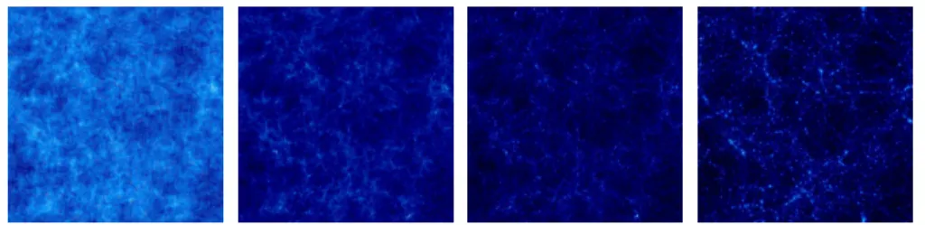
RAMSES2is a typical computational intensive application used by astrophysicists to study the formation of galaxies. RAMSESis used, among other things, to simulate the evolution of a collisionless, self-gravitating fluid called “dark matter” through cosmic time (see Fig-ure2). Individual trajectories of macro-particles are integrated using a state-of-the-art “N body solver”, coupled to a finite volume Euler solver, based on the Adaptive Mesh Refine-ment technics. The computational space is decomposed among the available processors using a mesh partitionning strategy based on the Peano–Hilbert cell ordering [12,13].

Figure 2: Time sequence (from left to right) of the projected density field in a cosmological simulation (large scale periodic box).

Cosmological simulations are usually divided into two main categories. Large scale periodic boxes (see Figure2) requiring massively parallel computers are performed on very long elapsed time (usually several months). The second category stands for much faster small scale “zoom simulations”. One of the particularity of the HORIZON3project is that it allows the re-simulation of some areas of interest for astronomers.

For example in Figure3, a supercluster of galaxies has been chosen to be re-simulated at a higher resolution (highest number of particules) taking the initial information and the boundary conditions from the larger box (of lower resolution). This is the latter category we are interested in. Performing a zoom simulation requires two steps: the first step consists of using RAMSES on a low resolution set of initial conditions i.e., with a small number of particles) to obtain at the end of the simulation a catalog of “dark matter halos”, seen in Figure2as high-density peaks, containing each halo position, mass and velocity. A small region is selected around each halo of the catalog, for which we can start the second step of the “zoom” method. This idea is to resimulate this specific halo at a much better resolution. For that, we add in the Lagrangian volume of the chosen halo a lot more particles, in order

Figure 3: Re-simulation on a supercluster of galaxies to increase the resolution

to obtain more accurate results. Similar “zoom simulations” are performed in parallel for each entry of the halo catalog and represent the main resource consuming part of the project. RAMSES simulations are started from specific initial conditions, containing the initial particle masses, positions and velocities. These initial conditions are read from Fortran binary files, generated using a modified version of the GRAFIC3code. This application

gen-erates Gaussian random fields at different resolution levels, consistent with current observa-tional data obtained by the WMAP4satellite observing the cosmic microwave background radiation. Two types of initial conditions can be generated with GRAFIC:

3_{http://web.mit.edu/edbert} 4_{http://map.gsfc.nasa.gov}

• single level: this is the “standard” way of generating initial conditions. The resulting files are used to perform the first, low-resolution simulation, from which the halo catalog is extracted.

• multiple levels: this initial conditions are used for the “zoom simulation”. The re-sulting files consist of multiple, nested boxes of smaller and smaller dimensions, as for Russian dolls. The smallest box is centered around the halo region, for which we have locally a very high accuracy thanks to a much larger number of particles. The result of the simulation is a set of “snaphots”. Given a list of time steps (or expan-sion factor), RAMSESoutputs the current state of the universe (i.e., the different parameters

of each particules) in Fortran binary files.

These files need post-processing with GALICSsoftwares: HaloMaker, TreeMaker and GalaxyMaker. These three softwares are meant to be used sequentially, each of them pro-ducing different kinds of information:

• HaloMaker: detects dark matter halos present in RAMSESoutput files, and creates a catalog of halos

• TreeMaker: given the catalog of halos, TreeMaker builds a merger tree: it follows the position, the mass, the velocity of the different particules present in the halos through cosmic time

• GalaxyMaker: applies a semi-analytical model to the results of TreeMaker to form galaxies, and creates a catalog of galaxies

Figure4shows the sequence of softwares used to realise a whole simulation.

5

Interfacing R

within D

5.1 Architecture of underlying deployment

The current version of RAMSESrequires a NFS working directory in order to write the out-put files, hence restricting the possible types of solving architectures. Each DIETserver will be in charge of a set of machines (typically 32 machines to run a 2563

particules simulation) belonging to the same cluster. For each simulation the generation of the initial conditions files, the processing and the post-processing are done on the same cluster: the server in charge of a simulation manages the whole process.

1

j+1

Retreiving simulation parameters Setting the MPI environment

RAMSES3d (MPI code)

TreeMaker : Post−processing

HaloMaker’s outputs GalaxyMaker : Post−processing Treemaker’s outputs 2 GRAFIC1: first run_{No zoom, no offset} 3 rollWhiteNoise : centering according to the offsets

cx, cy and cz 4 GRAFIC1: second run

with offsets If nb levels == 0 GRAFIC1 ... GRAFIC2 ... GRAFIC2 ... GRAFIC2 ... GRAFIC2 5’ 5" 5"’ 5n 6n 7n 8n jn 8"’ 7"’ 6"’ 6" 7" 6’ HaloMaker on 1 snapshot per process ... n

Stopping the environment Sending the post−processing to the client j+2’ j+2" j+2’’’ j+2 j+3 j+4 j+5

Figure 4: Workflow of a simulation

5.2 Server design

The DIETserver is a library. So the RAMSES server requires to define themain() func-tion, which contains the problem profile definition and registrafunc-tion, and the solving funcfunc-tion,

whose parameter only consists of the profile and named after the service name,solve_serviceName. The RAMSES solving function contains the calls to the different programs used for

the simulation, and which will manage the MPI environment required by RAMSES. It is

recorded during the profile registration.

The SED is launched with a call to diet_SeD()in the main() function, which will never return (except if some errors occur). The SED forks the solving function when

requested.

Here is the main structure of a DIETserver:

#include "DIET_server.h"

/* Defining the service function */ int solve_service(diet_profile_t *pb)

{ ... }

/* Defining the main function */ int main(int argc, char* argv[]) {

/* Initialize service table with the number of services */ /* Define the services’ profiles */

/* Add the services */

/* Free the profile descriptors */ /* Launch the SeD */

}

5.2.1 Defining services

To match client requests with server services, clients and servers must use the same prob-lem description. A unified way to describe problems is to use a name and define its arguments. The RAMSES service is described by a profile description structure called

diet_profile_desc_t. Among its fields, it contains the name of the service, an ar-ray which does not contain data, but their characteristics, and three integerslast_in, last_inoutandlast_out. The structure is defined inDIET_server.h.

The array is of size last_out + 1. Arguments can be:

IN: Data are sent to the server. The memory is allocated by the user.

INOUT: Data, allocated by the user, are sent to the server and brought back into the same memory zone after the computation has completed, without any copy. Thus free-ing this memory while the computation is performed on the server would result in a segmentation fault when data are brought back onto the client.

OUT: Data are created on the server and brought back into a newly allocated zone on the client. This allocation is performed by DIET. After the call has returned, the user

can find its result in the zone pointed by the value field. Of course, DIET cannot guess how long the user needs these data for, so it lets him/her free the memory with

The fields last_in, last_inout and last_out of the structure respectively point at the in-dexes in the array of the last IN, last INOUT and last OUT arguments.

Functions to create and destroy such profiles are defined with the prototypes below. Note that if a server can solve multiple services, each profile should be allocated.

diet_profile_desc_t *diet_profile_desc_alloc(const char* path, int last_in, int last_inout, int last_out); diet_profile_desc_t *diet_profile_desc_alloc(int last_in, int last_inout,

int last_out); int diet_profile_desc_free(diet_profile_desc_t *desc);

The cosmological simulation is divided in two services:ramsesZoom1andramsesZoom2, they represent the two parts of the simulation. The first one is used to determine interest-ing parts of the universe, while the second is used to study these parts in details. The

ramsesZoom2service uses nine data. The seven firsts are IN data, and contain the simu-lation parameters:

• a file containing parameters for RAMSES

• resolution of the simulation (number of particules) • size of the initial conditions (in M pc.h−1₎

• center’s coordinates of the initial conditions (3 coordinates: cx, cyand cz)

• number of zoom levels (number of nested boxes)

The last two are integers for error controls, and a file containing the results obtained from the simulation post-processed with GALICS. This conducts to the following inclusion in the server code (note: the same allocation must be performed on the client side, with the

diet_profile_tstructure):

/* arg.profile is a diet_profile_desc_t * */

arg.profile = diet_profile_desc_alloc("ramsesZoom2", 6, 6, 8);

Every argument of the profile must then be set withdiet_generic_desc_set()

defined inDIET_server.h, like:

diet_generic_desc_set(diet_parameter(pb,0), DIET_FILE, DIET_CHAR); diet_generic_desc_set(diet_parameter(pb,1), DIET_SCALAR, DIET_INT);

5.2.2 Registering services

Every defined service has to be added in the service table before the SED is launched. The complete service table API is defined inDIET_server.h:

typedef int (* diet_solve_t)(diet_profile_t *); int diet_service_table_init(int max_size);

int diet_service_table_add(diet_profile_desc_t *profile, NULL, diet_solve_t solve_func);

void diet_print_service_table();

The first parameter, profile, is a pointer on the profile previously described (section5.2.1). The second parameter concerns the convertor functionality, but this is out of scope of this paper and never used for this application. The parameter solve_func is the type of the

solve_serviceName()function: a function pointer used by DIETto launch the com-putation. Then the prototype is:

int solve_ramsesZoom2(diet_profile_t* pb) {

/* Set data access */ /* Computation */ }

5.2.3 Data management

The first part of the solve function (called solve_ramsesZoom2()) is to set data ac-cess. The API provides useful functions to help coding the solve function e.g., get IN arguments, set OUT ones, with diet_*_get()functions defined in DIET_data.h. Do not forget that the necessary memory space for OUT arguments is allocated by DIET.

So the user should call thediet_*_get()functions to retrieve the pointer to the zone his/her program should write to. To set INOUT and OUT arguments, one should use the

diet_*_desc_set()defined in DIET_server.h. These should be called within

“solve” functions only.

diet_file_get(diet_parameter(pb,0), NULL, &arg_size, &nmlPath); diet_scalar_get(diet_parameter(pb,1), &resol, NULL);

diet_scalar_get(diet_parameter(pb,2), &size, NULL); diet_scalar_get(diet_parameter(pb,3), &cx, NULL); diet_scalar_get(diet_parameter(pb,4), &cy, NULL);

diet_scalar_get(diet_parameter(pb,5), &cz, NULL); diet_scalar_get(diet_parameter(pb,6), &nbBox, NULL);

The results of the simulation are packed into a tarball file if it succeeded. Thus we need to return this file and an error code to inform the client whether the file really contains results or not. In the following code, the diet_file_set() function associates the DIETparameter with the current file. Indeed, the data should be available for DIET, when

it sends the resulting file to the client.

char* tgzfile = NULL;

tgzfile = (char*)malloc(tarfile.length()+1); strcpy(tgzfile, tarfile.c_str());

diet_file_set(diet_parameter(pb,7), DIET_VOLATILE, tgzfile);

5.3 Client

In the DIET architecture, a client is an application which uses DIET to request a service. The goal of the client is to connect to a Master Agent in order to dispose of a SED which will be able to solve the problem. Then the client sends input data to the chosen SED and, at the end of computation, retrieve output data from the SED. DIETprovides API functions to easily and transparently access the DIETplatform.

5.3.1 Structure of a client program

Since the client side of DIETis a library, a client program has to define themain() func-tion: it uses DIETthrough function calls. Here is the main structure of a DIETclient:

#include "DIET_client.h"

int main(int argc, char *argv[]) {

/* Initialize a DIET session */

diet_initialize(configuration_file, argc, argv); /* Create the profile */

/* Set profile arguments */ /* Successive DIET calls ... */

/* Retreive data */ /* Free profile */ diet_finalize(); }

The client program must open its DIETsession with a call todiet_initialize(). It parses the configuration file given as the first argument, to set all options and get a refer-ence to the DIETMaster Agent. The session is closed with a call todiet_finalize(). It frees all resources, if any, associated with this session on the client, servers, and agents, but not the memory allocated for all INOUT and OUT arguments brought back onto the client during the session. Hence, the user can still access them (and still has to free them !). The client API follows the GridRPC definition [10]: alldiet_functions are “dupli-cated” withgrpc_ functions. Bothdiet_initialize()/grpc_initialize()

anddiet_finalize()/grpc_finalize()belong to the GridRPC API.

A problem is managed through a function_handle, that associates a server to a service name. The returned function_handle is associated to the problem description, its profile, during the call todiet_call().

5.3.2 Data management

The API to the DIETdata structures consists of modifier and accessor functions only: no

allocation function is required, sincediet_profile_alloc()allocates all necessary memory for all argument descriptions. This avoids the temptation for the user to allocate the memory for these data structures twice (which would lead to DIETerrors while reading

profile arguments).

Moreover, the user should know that arguments of the_setfunctions that are passed by pointers are not copied, in order to save memory. Thus, the user keeps ownership of the memory zones pointed by these pointers, and he/she must be very careful not to alter it during a call to DIET. An example of prototypes:

int diet_scalar_set(diet_arg_t* arg,

void* value,

diet_persistence_mode_t mode,

int diet_file_set(diet_arg_t* arg, diet_persistence_mode_t mode,

char* path);

Hence arguments used in theramsesZoom2simulation are declared as follows:

// IN parameters

if (diet_file_set(diet_parameter(arg.profile,0), DIET_VOLATILE, namelist)) {

cerr << "diet_file_set error on the <namelist.nml> file" << endl; return 1;

}

diet_scalar_set(diet_parameter(arg.profile,1), &resol, DIET_VOLATILE, DIET_INT); diet_scalar_set(diet_parameter(arg.profile,2),

&size, DIET_VOLATILE, DIET_INT); diet_scalar_set(diet_parameter(arg.profile,3),

&arg.cx, DIET_VOLATILE, DIET_INT); diet_scalar_set(diet_parameter(arg.profile,4),

&arg.cy, DIET_VOLATILE, DIET_INT); diet_scalar_set(diet_parameter(arg.profile,5),

&arg.cz, DIET_VOLATILE, DIET_INT); diet_scalar_set(diet_parameter(arg.profile,6),

&arg.nbBox, DIET_VOLATILE, DIET_INT); // OUT parameters

diet_scalar_set(diet_parameter(arg.profile,8), NULL, DIET_VOLATILE, DIET_INT);

if (diet_file_set(diet_parameter(arg.profile,7), DIET_VOLATILE, NULL)) {

cerr << "diet_file_set error on the OUT file" << endl; return 1;

}

It is to be noticed that the OUT arguments should be declared even if their values is set to NULL. Their values will be set by the server that will execute the request.

Once the call to DIETis done, we need to access the OUT data. The 8th parameter is a file and the 9th is an integer containing the error code of the simulation (0if the simulation succeeded):

int* returnedValue; size_t tgzSize = 0; char* tgzPath = NULL;

diet_scalar_get(diet_parameter(simusZ2[reqID].profile,8), &returnedValue, NULL);

if (!*returnedValue) {

diet_file_get(diet_parameter(simusZ2[reqID].profile,7), NULL, &tgzSize, &tgzPath);

}

6

Experiments

6.1 Experiments description

Grid’50005 is the French Research Grid. It is composed of 9 sites spread all over France, each with 100 to 1000 PCs, connected by the RENATER Education and Research Network (1Gb/s or 10Gb/s). For our experiments, we deployed a DIETplatform on 5 sites (6 clus-ters).

• 1 MA deployed on a single node, along with omniORB, the monitoring tools, and the client

• 6 LA: one per cluster (2 in Lyon, and 1 in Lille, Nancy, Toulouse and Sophia) • 11 SEDs: two per cluster (one cluster of Lyon had only one SED due to reservation

restrictions), each controlling 16 machines (AMD Opterons 246, 248, 250, 252 and 275)

We studied the possibility of computing a lot of low-resolution simulations. The client requests a 1283particles 100M pc.h−1_{simulation (first part). When it receives the results, it}

requests simultaneously 100 sub-simulations (second part). As each server cannot compute more than one simulation at the same time, we won’t be able to have more than 11 parallel computations at the same time.

6.2 Results

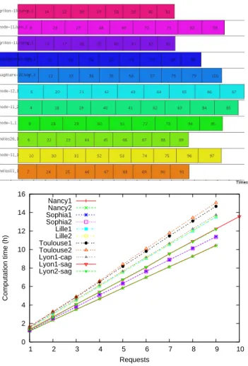
The experiment (including both the first and the second part of the simulation) lasted 16h 18min 43s (1h 15min 11s for the first part and an average of 1h 24min 1s for the second

part). After the first part of the simulation, each SED received 9 requests (one of them

received 10 requests) to compute the second part (see Figure5, left). As shown in Figure5

(right) the total execution time for each SED is not the same: about 15h for Toulouse and 10h30 for Nancy. Consequently, the schedule is not optimal. The equal distribution of the requests does not take into account the machines processing power. In fact, at the time when DIETreceives the requests (all at the same time) the second part of the simulation has never been executed, hence DIETdoesn’t know anything on its processing time, the best it can do

is to share the total amount of requests on the available SEDs. A better makespan could be attained by writing a plug-in scheduler[4].

The benefit of running the simulation in parallel on different clusters is clearly visible: it would take more than 141h to run the 101 simulation sequentially. Furthermore, the overhead induced by the use of DIET is extremely low. Figure 6 shows the time needed to find a suitable SED for each request, as well as in log scale, the latency (i.e., the time

needed to send the data from the client to the chosen SED, plus the time needed to initiate the service).

The finding time is low and nearly constant (49.8ms on average). The latency grows rapidly. Indeed, the client requests 100 sub-simulations simultaneously, and each SED cannot compute more than one of them at the same time. Requests cannot be proceeded until the completion of the precedent one. This waiting time is taken into account in the latency. Note that the average time for initiating the service is 20.8ms (taken on the 12 firsts executions). The average overhead for one simulation is about 70.6ms, inducing a total overhead for the 101 simulations of 7s, which is neglectible compared to the total processing time of the simulations.

7

Acknowledgment

This work was developed with financial support from the ANR (Agence Nationale de la Recherche) through the LEGO project referenced ANR-05-CIGC-11.

8

Conclusion

In this paper, we presented the design of a DIETclient and server based on the example of cosmological simulations. As shown by the experiments, DIETis capable of handling long

cosmological parallel simulations: mapping them on parallel resources of a grid, executing and processing communication transfers. The overhead induced by the use of DIET is ne-glectible compared to the execution time of the services. Thus DIETpermits to explore new

0 2 4 6 8 10 12 14 16 1 2 3 4 5 6 7 8 9 10 Computation time (h) Requests Nancy1 Nancy2 Sophia1 Sophia2 Lille1 Lille2 Toulouse1 Toulouse2 Lyon1-cap Lyon1-sag Lyon2-sag

Figure 5: Simulation’s distribution over the SEDs: at the top, the Gantt chart; at the bottom, the execution time of the 100 sub-simulations for each SED

research axes in cosmological simulations (on various low resolutions initial conditions), with transparent access to the services and the data.

Currently, two points restrict the ease of use of these simulations, and their performance: the whole simulation process is hard-coded within the server, and the schedule could be greatly improved. A first next step will be to use one of the latest DIETfeature: the workflow management system, which uses an XML document to represent the nodes and the data dependancies. The simulation execution sequence could be represented as a directed acyclic

40 50 60 70 80 90 100 110 120 130 0 20 40 60 80 1001 10 100 1000 10000 100000 1e+06 1e+07 1e+08

Finding time (ms) Latency (ms)

Request number Find Latency

Figure 6: Finding time and latency

graph, hence being seen as a workflow. A second step will be to write a plug-in scheduler, to best map the simulations on the available resources according to their processing power, to lower the unbalance observed between the SEDs. Finally, transparence could be added to the deployment of the platform, by using the DIET batch system. It allows to make transparent reservations of the resources on batch systems like OAR, and to run the jobs by submitting a script.

References

[1] A. Amar, R. Bolze, A. Bouteiller, P.K. Chouhan, A. Chis, Y. Caniou, E. Caron, H. Dail, B. Depardon, F. Desprez, J-S. Gay, G. Le Mahec, and A. Su. Diet: New developments and recent results. In CoreGRID Workshop on Grid Middleware (in conjunction with

EuroPar2006), Dresden, Germany, August 28-29 2006.

[2] D. Arnold, S. Agrawal, S. Blackford, J. Dongarra, M. Miller, K. Sagi, Z. Shi, and S. Vadhiyar. Users’ Guide to NetSolve V1.4. Computer Science Dept. Technical Report CS-01-467, University of Tennessee, Knoxville, TN, July 2001.

[3] Eddy Caron and Frédéric Desprez. Diet: A scalable toolbox to build network enabled servers on the grid. International Journal of High Performance Computing

[4] A. Chis, E. Caron, F. Desprez, and A. Su. Plug-in scheduler design for a distributed grid environment. In ACM/IFIP/USENIX, editor, 4th International Workshop on

Mid-dleware for Grid Computing - MGC 2006, Melbourne, Australia, November 27th

2006. To appear. In conjunction with ACM/IFIP/USENIX 7th International Middle-ware Conference 2006.

[5] A. Denis, C. Perez, and T. Priol. Towards high performance CORBA and MPI mid-dlewares for grid computing. In Craig A. Lee, editor, Proc. of the 2nd International

Workshop on Grid Computing, number 2242 in LNCS, pages 14–25, Denver,

Col-orado, USA, November 2001. Springer-Verlag.

[6] H. Nakada, M. Sato, and S. Sekiguchi. Design and implementations of ninf: towards a global computing infrastructure. Future Generation Computing Systems,

Metacom-puting Issue, 15:649–658, 1999.

[7] H. Nakada, Y. Tanaka, S. Matsuoka, and S. Sekiguchi. The Design and Implementa-tion of a Fault-Tolerant RPC System: Ninf-C. In Proceeding of HPC Asia 2004, pages 9–18, 2004.

[8] M. Sato, T. Boku, and D. Takahasi. OmniRPC: a Grid RPC System for Parallel Pro-gramming in Cluster and Grid Environment. In Proceedings of CCGrid2003, pages 206–213, Tokyo, May 2003.

[9] K. Seymour, C. Lee, F. Desprez, H. Nakada, and Y. Tanaka. The End-User and Middle-ware APIs for GridRPC. In Workshop on Grid Application Programming Interfaces,

In conjunction with GGF12, Brussels, Belgium, September 2004.

[10] Keith Seymour, Hidemoto Nakada, Satoshi Matsuoka, Jack Dongarra, Craig Lee, and Henri Casanova. Overview of GridRPC: A Remote Procedure Call API for Grid Com-puting. In Grid Computing - Grid 2002, LNCS 2536, pages 274–278, November 2002. [11] S. Shirasuna, H. Nakada, S. Matsuoka, and S. Sekiguchi. Evaluating Web Services Based Implementations of GridRPC. In Proceedings of the 11th IEEE International

Symposium on High Performance Distributed Computing (HPDC-11 2002), pages

237–245, July 2002.

[12] R. Teyssier. Cosmological hydrodynamics with adaptive mesh refinement. A new high resolution code called RAMSES. Astronomy and Astrophysics, 385:337–364, 2002. [13] R. Teyssier, S. Fromang, and E. Dormy. Kinematic dynamos using constrained

trans-port with high order Godunov schemes and adaptive mesh refinement. Journal of

[14] Y. Tanaka and H. Takemiya and H. Nakada and S. Sekiguchi. Design, Implementation and Performance Evaluation of GridRPC Programming Middleware for a Large-Scale Computational Grid. In Proceedings of 5th IEEE/ACM International Workshop on

Grid Computing, pages 298–305, 2005.

[15] A. YarKhan, K. Seymour, K. Sagi, Z. Shi, and J. Dongarra. Recent developments in gridsolve. In Y Robert, editor, International Journal of High Performance Computing

Applications (Special Issue: Scheduling for Large-Scale Heterogeneous Platforms),

4, rue Jacques Monod - 91893 ORSAY Cedex (France)

Unité de recherche INRIA Lorraine : LORIA, Technopôle de Nancy-Brabois - Campus scientifique 615, rue du Jardin Botanique - BP 101 - 54602 Villers-lès-Nancy Cedex (France)

Unité de recherche INRIA Rennes : IRISA, Campus universitaire de Beaulieu - 35042 Rennes Cedex (France) Unité de recherche INRIA Rocquencourt : Domaine de Voluceau - Rocquencourt - BP 105 - 78153 Le Chesnay Cedex (France)

Unité de recherche INRIA Sophia Antipolis : 2004, route des Lucioles - BP 93 - 06902 Sophia Antipolis Cedex (France)

Éditeur