HAL Id: hal-01635459
https://hal.archives-ouvertes.fr/hal-01635459
Submitted on 15 Nov 2017
HAL is a multi-disciplinary open access
archive for the deposit and dissemination of
sci-entific research documents, whether they are
pub-lished or not. The documents may come from
L’archive ouverte pluridisciplinaire HAL, est
destinée au dépôt et à la diffusion de documents
scientifiques de niveau recherche, publiés ou non,
émanant des établissements d’enseignement et de
Incremental Reconstruction of Manifold Surface from
Sparse Visual Mapping
Shuda Yu, Maxime Lhuillier
To cite this version:
Shuda Yu, Maxime Lhuillier. Incremental Reconstruction of Manifold Surface from Sparse Visual
Mapping. joint 3DIM/3DPVT Conference (3D Imaging, Modeling, Processing, Vizualization and
Transmission), Oct 2012, Zurich, Switzerland. �10.1109/3DIMPVT.2012.11�. �hal-01635459�
Incremental Reconstruction of Manifold Surface from Sparse Visual Mapping
Shuda Yu and Maxime Lhuillier
Institut Pascal, UMR 6602, CNRS/UBP/IFMA, Aubi`ere, France
[email protected]
This paper is accepted at 3DIMPVT’12 (DOI 10.1109/3DIMPVT.2012.11, Copyright 2012 IEEE).
Abstract
Automatic image-based-modeling usually has two steps: Structure from Motion (SfM) and the estimation of a trian-gulated surface. The former provides camera poses and a sparse point cloud. The latter usually involves dense stereo. From the computational standpoint, it would be nice to avoid dense stereo and estimate the surface from the sparse cloud directly. Furthermore, it would be useful for online applications to update the surface while the camera is mov-ing in the scene. This paper deals with both requirements: it introduces an incremental method which reconstructs a surface from a sparse cloud estimated by incremental SfM. The context is new and difficult since we ensure the resulting surface to be manifold at all times. The manifold property is important since it is needed by differential operators in-volved in surface refinements. We have experimented with a hand-held omnidirectional camera moving in a city.
1. Introduction
The estimation of the scene surface viewed by a camera is an important requirement for applications such as aug-mented reality, collision detection while moving along a planned path, environment modeling etc. However, the ma-jority of methods which produce a 2-manifold (e.g. dense multi-view stereo [19] or methods based on [10]) are batch methods. They are not easy to adapt to the incremental con-text where a surface is computed at all times from the pro-gressive availability of images or 3d points.
In a 2-manifold (i.e. 2d topological manifold surface), each point of the surface has a surface neighborhood which is homeomorphic to a disk. Thus, a triangulated 2-manifold is not a simple soup of badly connected triangles. Each triangle is exactly connected by its 3 edges to 3 other tri-angles, the surface has neither holes nor self-intersections, and it cuts R3into free-space and matter regions. Here we assume that the 2-manifold is triangulated.
The manifold property provides the possibility of esti-mating safely the differential operators [14] (e.g. curvature)
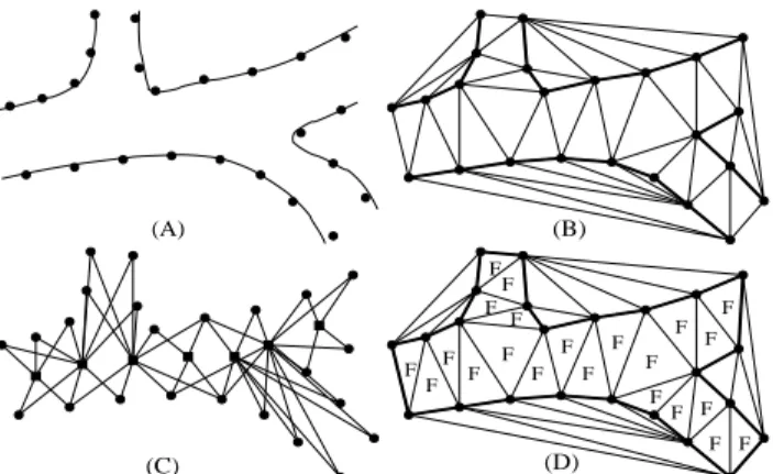
(C) (A)
(B) (D)
Figure 1. (A) is a denoised non-manifold, (B) is a non-denoised 2-manifold, (C) is a denoised 2-manifold, (D) is the texture of (C). In (A,B,C), the triangle normals are encoded by colors.
used by surface refinements like surface fairing and dense stereo. In this paper, we use a surface denoising based on discrete Laplacian [20], whose performances are degraded if we apply it on a non-manifold surface. Fig. 1 shows an example for car and street (during winter) reconstructed by our methods from a sparse SfM point cloud. More gener-ally, a lot of Computer Graphic algorithms do not apply if the triangle list is not a 2-manifold [4].
Note that a 2-manifold directly estimated from the sparse cloud produced by SfM would be ideal for both time and space complexities. This surface would also be useful for initializing a more accurate (but more costly) surface recon-struction method such as surface deformation minimizing photo-consistency [8, 17]. The dense-stereo/deformation step is outside the scope of this paper.
To our knowledge, this paper presents the first incremen-tal method which provides a 2-manifold from a sparse cloud of reconstructed interest points provided by SfM. Here “in-cremental” means that a 2-manifold obtained before time
t is locally updated using 3d points provided by SfM at t to obtain the 2-manifold at t. SfM is also incremental:
the geometry att (camera poses and sparse point cloud of
the sequence up tot) is a local update of a geometry
be-foret. We focus on the mapping scenario such as a
cam-era mounted on vehicle/robot/human exploring an unknown and large scene. In our experiments, a hand-held
omnidirec-(A) (B) (C) F F F F F F F F F F F F F F F F F F F F F F (D)
Figure 2. In the 2d case, surfaces, tetrahedra and triangles are re-placed by curves, triangles and edges, respectively. (A) curves to be reconstructed and points which sample the curves. (B) the De-launay triangulation of the points (the bold-faced DeDe-launay edges approximate the curves). (C) points (circle) and camera locations (squares) linked by rays (segments). (D) the Delaunay triangles in-tersected by rays are free-space and are denoted by “F”. The other triangles are matter. The Delaunay edges separating free-space and matter are bold-faced.
tional (calibrated) video camera is moving in a city. This is different to the scenario of a camera moving in a limited workspace such as desk-like/indoor environments [17].
Section 2 compares our work against others. Sections 3 and 4 describe a batch method [22] and our incremental method, respectively. The former is useful to describe the latter. Lastly, the experiments and conclusion are given in Sections 5 and 6.
2. Previous Work
We discuss the previous works which reconstruct a sur-face from sparse (not dense) cloud of features reconstructed by SfM. Since most of these methods use a 3d Delaunay triangulation, we start with a reminder of what this is.
A lot of surface reconstruction methods [5] are based on the following property [2]: ifP is a sufficiently dense
sam-ple of points on the (smooth) scene surface, a good approx-imation of this surface is given by a list of triangles of the 3d Delaunay triangulationT of P . T is a list of tetrahedra
which partitions the convex hull ofP such that (1) the
ver-tices of all tetrahedra areP and (2) the tetrahedra
circum-spheres do not contain a vertex within them. The triangles are the facets of the tetrahedra. Fig. 2 (A and B) illustrates this property in the 2d case.
In our case, the points are reconstructed from images and we know the listViof indices of images which reconstruct the 3d point pi ∈ P . We refer to a ray as a line segment
linking pito thej-th camera location cjsuch thatj ∈ Vi.
The free-space carving methods [6, 11, 18, 13, 22] use rays as visibility constraints to label the tetrahedra of a 3d Delaunay: a tetrahedron is free-space if it is intersected by at least one ray, otherwise it is matter. These methods deal
with sparse cloud of points (or edges [6]), and only [13] is incremental. They (except [6] and [22]) directly consider the surface as the list of triangles separating the free-space and matter tetrahedra (see Fig. 2). Unfortunately, the result-ing surface may be non-manifold. For example, the surface has a singularity at vertex v if all tetrahedra which have ver-tex v are matter, except two free-space tetrahedra∆1and
∆2 such that the intersection of∆1 and∆2 is exactly v. In [6] ([22], respectively), a region growing procedure in the list of matter (free-space, respectively) tetrahedra removes all singularities and provides a 2-manifold.
Methods [15, 21, 9] use 2d Delaunay triangulations and deal with a sparse cloud of features. Only [9] is incremental, but the surface is not manifold (it may have holes) and the approach is applied to a small sequence of real images.
3. Batch Surface Reconstruction
The batch method is useful to describe our incremental method. Its steps are 3d Delaunay, Ray tracing, 2-Manifold Extraction, Topology Extension, and Surface Denoising.
3d Delaunay Triangulation T Assume that SfM esti-mates the geometry of the whole image sequence. The ge-ometry includes the sparse cloud of points {pi}, camera
locations{cj} and rays defined by visibility lists {Vi}
(no-tations in Section 2). Point pi has poor accuracy if it is
reconstructed in degenerate configuration [7]: if piand all cj, j ∈ Viare nearly collinear. This case occurs in part of the camera trajectory which is a straight line and if points reconstructed from this part are close to the straight line. Thus, piis added inT if and only if there is an angle \cjpick
(j, k ∈ Vi) larger than thresholdǫ.
We also add extra points inT . For the clarity of our
cur-rent paper, we only mention that (1) these extra points act reconstructed points with empty visibility lists and (2) they are randomly added in the neighborhood of the camera tra-jectory. The reason (removal of spurious arks/handles) and technical details are in Section 4 of our previous paper [22].
Ray Tracing As all tetrahedra are initialized matter, ray-tracing is applied to each ray to force into free-space all tetrahedra intersected by the ray. T is defined by a graph:
a graph vertex is a tetrahedron, a graph edge is a triangle between two tetrahedra. Tracing a ray cjpi is a walk in
the graph, starting from the tetrahedron which contains cj,
moving to another tetrahedron through the triangle inter-sected by the line segment cjpi, stopping in tetrahedron
which has vertex pi. Now we know the label (matter or
free-space) of all tetrahedra which partition the convex hull
C of the points, but the label of R3\ C is unknown. In our
case, the points are reconstructed in almost all directions around view points (we reconstruct an environment). Thus,
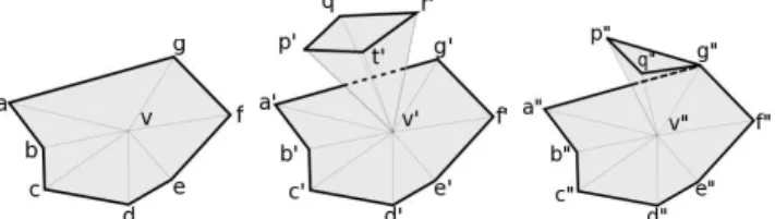
Figure 3. v is regular since the edges opposite to v define
a simple polygon abcdef ga on the surface. v′ and v′′ are
not regular since polygons a′b′c′d′e′f′g′a′
− p′q′r′t′p′ and a′′b′′c′′d′′e′′f′′g′′p′′q′′g′′a′′are not simple (the former is not con-nected, the latter has multiple vertex g′′).
view points and rays are in the convex hull of the points. Since the rays do not intersect R3\ C, R3\ C is matter.
2-Manifold Test The target surfaceS is a list of triangles
ofT which should be 2-manifold. Let v be a point in S.
We say that v is regular if it has a neighborhood inS which
is topologically a disk. Otherwise v is singular. By defi-nition,S is 2-manifold if all its points are regular. In our
context whereS is a list of triangles of T , it is sufficient to
check that each vertex v ofS is regular using the following
neighborhood of v: the list of theS triangles which have
vertex v [3]. Then, v is regular if and only if the edges op-posite to v in the triangles ofS having v as vertex form a
simple polygon (Fig. 3). A simple polygon is topologically a circle, i.e. a list of segments which forms a closed path without self-intersection.
2-Manifold Extraction The target surfaceS should also
separate free-space and matter as far as possible, under the constraint that it is 2-manifold. A 2-manifold cuts R3in re-gions labeled outside (outside the matter) and inside. Here the outside region O contains a maximum of free-space
tetrahedra and does not contain matter tetrahedron. A re-gion growing process is used: O grows from ∅ by adding
free-space tetrahedra one by one, such that the border δO
ofO remains 2-manifold. The final δO is S. We know that δO is 2-manifold if and only if all δO vertices are regular.
Since tetrahedra are added one by one, the neighborhoods of at most four vertices ofδO (those of the added
tetrahe-dron) are modified. So we only need to check that these vertices are regular after the tetrahedron is added. If this is not the case, this tetrahedron is removed fromO and we try
another one. The finalO depends on the addition order of
the tetrahedra inO. We choose the added free-space
tetra-hedron such that it has a facet included inδO, i.e. it is in
the neighborhood ofO. A priority is also defined for each
free-space tetrahedron: the number of rays which intersect the tetrahedron. The tetrahedra in the neighborhood of O
are stored in a heap (priority queue) for fast selection of the tetrahedron with the largest priority.
The inputs of the region growing are the initialO, the set F0of tetrahedra where the growing is possible, the setQ0of
tetrahedra which includes the initial value of the heap, and function r which maps a tetrahedron ∆ to the number of
rays which intersect∆. In the batch case, O = ∅, Q0= T
andF0is the list of free-space tetrahedra ofT . The output
isO. Here is the algorithm in C style.
// **** initialization of priority queue (heap)Q **** Q = ∅;
if (O==∅) { // used by batch algo.
let∆ ∈ F0be such thatr(∆) is maximum; Q ← Q ∪ {∆};
} else // used by topology extension and incremental algo.
for each tetrahedron∆ in Q0∩ F0
if (∆ /∈ O and one of its 4 neighbors is in O) Q ← Q ∪ {∆};
// **** region growing ofO ****
while (Q!=∅) {
pick fromQ the ∆ which has the largest r(∆);
if (∆ ∈ O) continue; O ← O ∪ {∆};
if (all vertices of∆ are regular) { // read the Appendix
for each∆′in the list of the four∆ neighbors
if (∆′ ∈ F0and∆′∈ O) Q ← Q ∪ {∆/ ′}; } else O ← O \ {∆};
}
Topology Extension TheδO genus can not be changed if
the tetrahedra are added one by one by the algorithm above:
O always has the ball topology. This is problematic if the
true outside does not have the ball topology, e.g. if the cam-era trajectory contains closed loop(s) around building(s). In the simplest case of one loop, the true outside has the toroid topology and the computed outsideO can not close
the loop. This problem is corrected as follows. First, we find a vertex inδO such that all inside tetrahedra incident to
this vertex are free-space. Second, we force all these tetra-hedra to outside (O is increased). Third, we check that all
vertices of these tetrahedra are regular. In case of failure(s), these tetrahedra are restored to inside (O is decreased).
Fi-nally, we alternate this scheme and the previous algorithm until no more tetrahedron can be added inO. Here, Q0is the list of tetrahedra neighbors of the forced tetrahedra above, andF0is unchanged.
Surface Denoising TheS reconstruction noise is reduced
thanks to a smoothing filter p′ = p + ∆p where p is a
vertex of S and ∆p is a discrete Laplacian defined on S
vertices [20]. The smoothed p′ is stored in a distinct array
of p. We don’t apply p ← p′ to avoid the computation
4. Incremental Surface Reconstruction
Our method is defined by a main loop which alternates the incremental versions of the steps in Section 3. Integert
specifies the current time and the keyframe index.
Incremental SfM First, a new keyframe is selected from the input video and interest points are matched with the previous keyframe using correlation. The new keyframe is such that the number of its matches with the two previous keyframes is larger than a threshold. Then, the new pose is robustly estimated (using Grunert’s method and RANSAC) and new 3d points are reconstructed from the new matches. Lastly, local bundle adjustment refines the geometry of the
l-most recent keyframes. Using l = 3, the l most recent
keyframes aret − 2, t − 1 and t. No more details are given
on this SfM step since it is similar to [16].
3d Delaunay TriangulationT We add point p toT once preaches its final value by SfM. From the computational
standpoint, this is efficient since we don’t need to updateT
every time SfM updates p. More precisely, we add inT at
timet (after the SfM step at t) every 3d point p such that
its last track is in keyframet − 2. As in the batch case, we
check that p is not in a degenerate configuration and we add extra points. A fixed number of extra points is added in the neighborhood of ct.
Dating Our incremental method needs a creation date for all tetrahedra and vertices. Furthermore, we use the Delau-nay implementation of CGAL [1] which adds the points one by one toT . The adding of p destroys list Ld(p) of
tetrahe-dra and creates listLc(p) of other tetrahedra. So we assign
datet to p and to the tetrahedra of Lc(p) if p is added to T at time t. We also need the smallest date dtof all outside tetrahedra inLd(p) destroyed at time t (for all p added at t). Each tetrahedron was labeled outside or inside by the
2-manifold step below. Both listsLc(p) and Ld(p) are easy
to compute thanks to CGAL functions.
Ray Tracing Tracing all rays available at date t is too
time consuming. Here we do the following approximation: the label (free-space or matter) of a tetrahedron is defined by the rays which have creation dates similar to or greater than that of the tetrahedron. A ray has the creation date of its 3d point, defined in the “Dating” step. According to this approximation, we only need to ray-trace the most recent rays. At datet, we apply ray-tracing to the small list of rays
which have creation dates in{t − k, · · · , t − 1, t}, where k
is a threshold.
2-Manifold Extraction Starting the region growing from
O = ∅ as in the batch case is too time consuming. In the
Figure 4. Region growing for image t = 98. The number of tetra-hedra layers contained in a pack is n = 20. Left: before region growing for image 98, the 2-manifolds of layers 20, 40, 60, 80 and 97 are already computed. Left-middle: point insertion destroys tetrahedra. The earliest creation date of tetrahedra which are
de-stroyed due to point additions in T is dt = 51. Right-middle:
the 2-manifolds of layers 60, 80, and 97 are invalid and destroyed.
Right: region growing from layer ni0to layer 98 by pack of n.
incremental case, we propose a method which starts the re-gion growing from a listO obtained at a recent date. We
regroup the free-space tetrahedra into different layers Lt′
by creation date t′ and the idea of growing the outsideO
by layer of creation date comes naturally to mind. We grow
O layer by layer, and for each layer, only free-space
tetra-hedra created before or at this layer can be added into O.
As a result, for each layer, we could extract a 2-manifold as the border of the tetrahedra list O. Then the 2-manifold
of the next layer can be easily computed by starting from that of the current layer. In practice, we prefer to grow by pack ofn layers for efficiency. At each time t, the method
holds several lists of outside tetrahedra which correspond to particular creation dates (multiples ofn): On,O2n, ...Oitn
whereitis the largest integer such thatitn ≤ t. These lists
and another listOtof outside tetrahedra meet
On⊆ O2n⊆ · · · ⊆ O(it−1)n⊆ Oitn ⊆ Ot
∀t′∈ {n, 2n, · · · , itn, t}, Ot′ ⊆ L1∪ L2∪ · · · ∪ Lt′
and the border ofOt′ is 2-manifold. (1)
The border ofOtis the target 2-manifoldS at time t.
Fur-thermore, the region growing at timet + 1 is started from
one of theOt′lists above.
To simplify notations in this Section, timet starts from 1 (not 0) and we define O0 = ∅. If t ≤ n, we apply the
batch region growing in all free-space tetrahedra from O0
to obtainOt. Now assume thatt > n. The algorithm works
from Eq. 1 att − 1 to Eq. 1 at t. Fig. 4 illustrates this if t = 98, n = 20, dt = 51. Remember that the point
addi-tions at timet destroy tetrahedra and we know the smallest
date dt of the destroyed outside tetrahedra. Leti0 be the largest integer such that i0n < dt. Ifi ≤ i0, Oin is un-changed and its border is still manifold. Ifi0< i, tetrahedra
may be destroyed inOin, its border may be non manifold andOinshould be recomputed. Time starts from 1, thus 1 ≤ dt,0 ≤ i0andOi0nexists. Then we apply region
grow-ing (2-manifold extraction in Section 3) fromOi0nto obtain
O(i0+1)n. We also apply region growing fromO(i0+1)nto
obtainO(i0+2)nand so on, until we obtainOitn. Lastly, we
apply region growing fromOitnto obtainOt. Remember
thatF0 andQ0 should also be defined for region growing fromOinto obtainO(i+1)n (orOt), as mentioned in
Sec-tion 3. For time complexity reason, we don’t useQ0 = T
but the most recent layers Q0 = Lin−b0 ∪ · · · ∪ L(i+1)n
whereb0 ∈ N is constant. We also define F0by the free-space tetrahedra ofL(i0−1)n∪ · · · ∪ L(i+1)n(not those of
L0∪ · · · ∪ L(i+1)n).
Topology Extension TheOin(includingOt) obtained at the previous step are improved by an incremental version of “Topology Extension” (Section 3) after the region growing fromO(i−1)n toOin. The improvedOinstill meet Eq. 1. “Topology Extension” is only applied to the most recent vertices ofS which have creation dates in − b1, · · · , in − 1, in where b1 ∈ N is a threshold. These vertices are only
tried once (there is only one “2-Manifold Extraction” and one “Topology Extension” for a giveni). Here we use Q0
of Section 3 andF0 is the list of free-space tetrahedra of
L(i0−1)n∪ · · · ∪ Lin.
Surface Denoising Denoising all vertices of S is too
time consuming. In the incremental case, we only need to smooth vertex p ofS if its smoothing p′at timet is
differ-ent to that att − 1 due to the steps above. As in Section 3,
the smoothing is p′ = p + ∆p where ∆p only depends
on p andN (p). Neighborhood N (p) is the list of vertices
which are connected to p by an edge ofS. Thus p′is
(re)-calculated if p is a new vertex ofS or if N (p) changes at t.
The tetrahedra listOt\Oi0nis the outside volume grown by
steps “2-Manifold Extraction” and “Topology Extension” att. Furthermore, all S changes at t are on the border of Ot\ Oi0n. So we (re)-calculate p′ifN (p) ∪ {p} contains
at least one vertex of the border ofOt\ Oi0n.
5. Experiments
5.1. Synthetic Sequence
Here we compare the performances of the batch (Sec-tion 3) and the incremental (Sec(Sec-tion 4) surface reconstruc-tion methods on the same sparse cloud of 3d points esti-mated from images of a synthetic scene. The synthetic scene is manually generated from real images taken in a city. The trajectory is a 230 m long closed loop around a building including several shops. The images are generated by ray-tracing and taking into account the ray reflection on the mirror. The catadioptric camera has axial symmetry. The large circle, which contains the scene projection in the image, has a 600 pixel radius. Fig. 5 (top-left corner) shows two images of the synthetic sequence.
SfM [12] reconstructs 600 camera poses and a sparse
cloud of257336 3d points from the sequence. We
approx-imate the true calibration by a central model and refine the radial distortion parameters using bundle adjustment. We estimate the similarity transformationR which minimizes E(R) =P599i=0||R(ci) − cgi||2, where ciand cgi are the
es-Figure 5. Two omnidirectional images, the sparse point cloud (and camera trajectory) by SfM, the batch surface, the final incremental surface. We remove the triangles on the sky to make viewing in the figure easier.
timated locations and the ground truth locations of the cam-era, respectively (ciis at the camera center and c
g
i is at the
mirror apex). We foundpE(R)/600 = 5.1 cm and use R to map the estimated geometry (poses and point cloud) in the ground truth coordinate system.
Both batch and incremental methods select points using
ǫ = 10 degrees and add 2 extra points in the neighborhood
of every ct(3d Delaunay Triangulation step). The
incre-mental method has parametersk = 40 (Ray-Tracing step), n = 60 and b0 = 10 (2-Manifold Extraction step), b1= 10
(Topology Extension step).
Qualitative Comparison Before using the ground truth, it is interesting to compare batch and incremental results. The 3d Delaunay triangulation has 123196 vertices and 750219 tetrahedra. The numbers of free-space tetrahedra are 494562 for batch and 490174 for incremental (the dif-ference is 0.9%). The batch and incremental (final) surfaces have 233273 and 231826 triangles, respectively.
Remember that the listO of outside tetrahedra grows in
the list of free-space tetrahedra. Thus the ratio between the numbers of outside and free-space tetrahedra can be used to compare the performances of the growing steps (2-Manifold Extraction and Topology Extension). Batch sur-face has 89.1% and incremental (final) sursur-face has 85.8%. We explain this results as follows: the incremental growing is more constrained than the batch growing. In the incre-mental case, both dating and manifold constraints are used. The batch method only uses manifold constraints. In
prac-Table 1. Errors of batch and incremental (final) surfaces using ground truth surface. The numbers between parentheses are ob-tained for twice smaller images.
method inliers (%) median (cm) 90% quantile (cm) batch 75.7 (73.9) 8.0 (64.3) 55 (103) increm. 72.4 (69.7) 8.6 (71.0) 50 (106)
tice, the ratio can not reach 100% since ray-tracing alone does not enforce the manifold constraint between free-space and matter tetrahedra.
Quantitative Comparison Now we define an error func-tion to compare the estimated surface (batch or incremental) against the ground truth surface. At first glance, we could use distancee(p) between the ground truth surface and
vtex p of the estimated surface [19]. Unfortunately, this er-ror is biased in favor of reconstructed areas which have the largest densities of reconstructed points (ground parts have low textures and densities, walls have high densities). A second idea is the use of the same error such that p samples uniformly the estimated surface. However, this method has drawback since the closest point in the ground truth surface does not necessarily correspond to the same point p.
Our solution does not have the problems above. Let q be a pixel in an image of the sequence. Let pebe the
intersec-tion of the estimated surface and the back-projected ray of
qby the estimated camera pose. Let pgbe the intersection
of the ground truth surface and the back-projected ray of q by the ground truth camera pose. In both cases, if there are several intersections, we take the intersection which is the closest to the camera pose. Then we usee(q) = ||pe−pg||.
If pgdoes not exist ore(q) > µ0(whereµ0= 2 m), we
as-sume that the point matching(pe, pg) is outlier (e.g. for the
pixels of the sky) and we ignore the error for q. In practice, we estimate the statistic ofe(q) by uniform sampling of q
in all images of the sequence. We sample 6000000 pixels in the sequence. Tab. 1 provides the results for both batch and incremental methods. We see that the batch method has slightly better results than the incremental method.
Lastly, the same experiment (both SfM and surface cal-culations) is re-done for the same images down-sampled by 2. We foundpE(R)/600 = 56 cm, which implies that the SfM drift is larger than in the previous case. According to Tab. 1, the batch surface is still the best and the surface ac-curacies are degraded. Fig. 5 shows the sparse point cloud by SfM and the surfaces.
5.2. Real Sequence
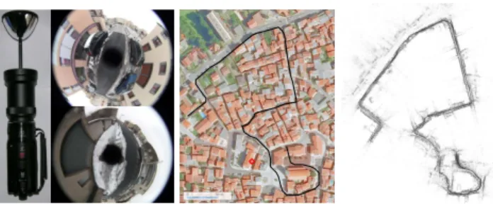
Our (equiangular) calibrated catadioptric camera is the 0-360 mirror mounted on the Canon Legria HSF10. We take a 1920*1080 AVCHD (MP4) video walking in a city
Figure 6. From left to right: our hand-held camera, two images of the sequence, aerial view of the trajectory, the sparse point cloud reconstructed by incremental SfM.
Figure 7. Images of the incremental surface reconstruction (also in the joint video). Top: gray levels encode the triangle normals. Bottom: one omnidirectional image is used for texture mapping. The black areas are due to triangles without texture in this image.
during 505 seconds and pointing the mirror toward the sky by hand. Ground truth is not available, but we know that the trajectory length is about 800 m. The view field is 360 de-grees in the horizontal plane and 51-58 dede-grees above and below. Fig. 6 shows our camera and several images of the sequence. The horizontal and vertical radii of the large el-lipse, which contains the scene projection in the images, are 700 and 693 pixels, respectively.
The method in Section 4 is applied to the (down-sampled by 2) images with the same parameters as in Section 5.1. 1033 keyframes are selected from 25278 images. About 600 Harris points are matched by correlation in three con-secutive keyframes. Fig. 6 shows the 187588 reconstructed points by incremental SfM for the complete sequence. The SfM drift is also visible thanks to an aerial photography (un-used by our method).
Fig. 7 shows the surface obtained at five different timest.
The observer moves in the scene such that he/she is observ-ing the most recent part of the surface at a (roughly) con-stant distance. This part is mainly within a ball whose center is ct−2att. At time t, the observer is located at ct−20and is looking towards ct−2. The observer and the surface end come forward simultaneously. These images are extracted from the joint video at http://maxime.lhuillier.free.fr.
Fig. 8 shows one global view and two local views of the last surface, which has 234354 triangles and 117145 ver-tices. 89.3% of free-space tetrahedra are outside tetrahedra. Remember that the surface is closed, so it also models the sky. In the figure, we remove the triangles on the sky to make viewing easier. Also we note that enforcing the
man-Figure 8. Views of the incremental (final) surface.
ifold constraint is not an option. If we simply define the final surfaceS by the list of triangles between free-space
and matter tetrahedra, we find that 25.5% of theS vertices
are not regular. Fig. 1 shows that this degrades the quality. Fig. 9 (on the left) shows the computation times of
the different steps at each time t: “Delaunay” in
yel-low (3d Delaunay Triangulation+Dating), “Carving” in blue (Ray Tracing), “Manifold” in red (2-Manifold Ex-traction+Topology Extension), “Post-processing” in green (Surface Denoising) and “Total” in black. We use a Core 2 Duo E8500 at 3.16 GHz. About 121 points per time
are added to the 3d Delaunay triangulation. “Delaunay” and “Post-processing” have almost negligible computation times in comparison to the other steps. “Carving” is less than 190 ms. Ift ∈ [0, 925], “Manifold” is less than 200 ms.
In the other cases, “Manifold” is between 50 and 600 ms. Thanks to Fig. 9 (on the right), we see that the compu-tation times of “Manifold” and “Post-Processing”globally increase if t − dtincreases and t − dt > 50. .
Further-more,t − dt< 280 in the whole sequence. Remember that dt is the smallest date of all outside tetrahedra destroyed at timet by “Delaunay”. These results are consistent with
those of a theoretical time complexity study: Delaunay and Carving are O(1), Manifold is O((t − dt) log(t − dt)),
Post-Processing is O(t − dt). Actually, these tight bounds should be considered as conjectures since the proofs use strong as-sumptions and will be submitted in another paper.
We now explain the large values of “Manifold” if t ∈ [925, 1032]. In a complete trajectory loop, vertices added at
the loop end (at timet) destroy outside tetrahedra created
at the loop beginning (at time dt) since these vertices and tetrahedra have similar 3d locations. The larger the loop, the largert − dt, and the larger the “Manifold” (and “Post-Processing”) computation time. Fig. 6 shows that the recon-structed trajectory has two incomplete (about 75%) loops: a large one on the top and a small one on the bottom. Here the loops are incomplete but the same principle applies for the small loop which is 75% closed ift ∈ [925, 1032]: there are
times in [925, 1032] such that added vertices destroy
out-side tetrahedra created at the loop beginning. This does not apply in the large loop case since (1) the added vertices and outside tetrahedra are in a tubular neighborhood of the cam-era trajectory and (2) the neighborhood radius is less than the (divided by 2) distance between both ends of the loop. Fig. 8 shows the neighborhood and its size; the small loop is on the top and the large loop on the bottom.
6. Conclusion
To our knowledge, this paper presents the first system with four features: incremental reconstruction for triangu-lated manifold surface from sparse point cloud generated by SfM. In experiments, we use a synthetic image sequence to compare and discuss the performance of our incremen-tal method and the related batch method. Although the batch method has slightly better results than our incremen-tal method, the latter is interesting for online applications that the former can not solve. We also reconstruct parts of a city using a hand-held omnidirectional camera and provide
Figure 9. Calculation times of the incremental surface reconstruction as a function of t (left) or a function of t − dt(right).
a detailed explanation of the computation times.
Several steps of the method can be improved and are sub-jects for future work. Image edges could be reconstructed and integrated in the Delaunay to improve the surface. The region-growing step should be accelerated in the case of a closed loop in the camera trajectory. Currently, the surface is denoised assuming that the point cloud is dense enough to estimate a discrete Laplacian. This improves the surface but it would be better to design a dedicated denoising method for sparse SfM point clouds. Lastly, we plan to use our method for online applications, larger data sets, and to ini-tialize surface reconstruction methods which are more time expensive and more accurate.
Appendix: Region Growing Acceleration
Here is a note to accelerate the “2-Manifold Extraction” step. In the algorithm of Section 3, we first insert tetrahe-dron∆ in O and then check if δO is 2-manifold. However,
we can do this faster (as in [3]) if we first check a condition on the neighborhood of∆ and then add ∆ to O (if the
con-dition is meet). Letf be the number of ∆ facets which are
inδO. If f = 1, ∆ is added to O if and only if the vertex
of∆, which is not in the δO facet, does not have adjacent
tetrahedron inO. If f = 0, ∆ is added to O if and only if the
four vertices meet this same condition. Iff = 2, ∆ is added
toO if and only if the edge of ∆, which is not an edge of
the twoδO facets, does not have adjacent tetrahedron in O.
Iff = 3 or f = 4, ∆ is added to O. In our implementation,
we greatly accelerate these computations by precalculating for each vertex the list of its adjacent tetrahedra.
References
[1] CGAL, www.cgal.org
[2] N. Amenta and M. Bern. Surface reconstruction by voronoi filtering. Discrete Computational Geometry, vol. 22, 1984. [3] J.D. Boissonnat. Geometric structures for three-dimensional
shape representation. ACM Transaction on Graphics, vol. 3, num. 4, p. 266-286, 1984.
[4] M. Botsch, L. Kobbelt, M. Pauly, P. Alliez, and B. Levy.
Poly-gon Mesh Processing. AK Peters, 2010.
[5] F. Cazals and J. Giesen. Delaunay triangulation based surface reconstruction: ideas and algorithms. INRIA technical report 5394, 2004.
[6] O. Faugeras, E. Le Bras-Mehlman, and J.D. Boissonnat. Rep-resenting stereo data with the delaunay triangulation. Artificial
Intelligence, p. 41-47, 1990.
[7] R. Hartley and A. Zisserman. Multiple View Geometry in
Computer Vision. C.U. Press, 2003.
[8] V.H. Hiep, R. Keriven, P. Labatut, and J.P. Pons. Towards high-resolution large-scale multi-view stereo. CVPR’09. [9] A. Hilton. Scene modelling from sparse 3d data. Image and
Vision Computing, vol. 23, p. 900-920, 2005.
[10] M. Kazhdan, M. Bolitho, and H. Hoppe. Poisson surface re-construction. Eurographics Symposium on Geometry
Process-ing, 2006.
[11] P. Labatut, J.P. Pons, and R. Keriven. Efficient multi-view reconstruction of large-scale scenes using interest points, De-launay triangulation and Graph-Cuts. CVPR’07.
[12] M. Lhuillier. Automatic scene structure and camera motion using a catadioptric camera. CVIU, 29(2), p. 186-203, 2008. [13] D. Lovi, N. Birkbeck, D. Cobzas, and M. Jagersand.
In-cremental free-space carving for real-time 3d reconstruction.
3DIMPVT’10.
[14] M. Meyer, M. Desbrun, P. Schroder, and A.H. Barr. Discrete differential-geometry operators for triangulated 2-manifolds.
Visualization and Mathematics III, 2003.
[15] D.D. Morris and T. Kanade. Image-consistent surface trian-gulation. CVPR’00.
[16] E. Mouragnon, M. Lhuillier, M. Dhome, F. Dekeyser, and P. Sayd. Generic and real-time structure from motion using local bundle adjustment. IVC, vol. 27, p. 1178-1193, 2009. [17] R.A. Newcombe and A.J. Davison. Live Dense
Reconstruc-tion with a Single Moving Camera. CVPR’10.
[18] Q. Pan, G. Reitmayr, and T. Drummond. ProFORMA: probabilistic feature-based on-line rapid model acquisition.
BMVC’09.
[19] S.M. Seitz, B. Curless, J. Diebel, D. Scharstein, and R. Szeliski. A comparison and evaluation of multi-view stereo reconstruction algorithms. CVPR’06.
[20] G. Taubin. A signal processing approach to fair surface de-sign. SIGGRAPH’95.
[21] C.J. Taylor. Surface reconstruction from feature based stereo.
ICCV’03.
[22] S. Yu and M. Lhuillier. Surface reconstruction of scenes us-ing a catadiopric camera. MIRAGE’11 (also in LNCS, volume 6930).