HAL Id: hal-02191369
https://hal-lara.archives-ouvertes.fr/hal-02191369
Submitted on 23 Jul 2019
HAL is a multi-disciplinary open access
archive for the deposit and dissemination of
sci-entific research documents, whether they are
pub-lished or not. The documents may come from
teaching and research institutions in France or
abroad, or from public or private research centers.
L’archive ouverte pluridisciplinaire HAL, est
destinée au dépôt et à la diffusion de documents
scientifiques de niveau recherche, publiés ou non,
émanant des établissements d’enseignement et de
recherche français ou étrangers, des laboratoires
publics ou privés.
The analysis of 6-component measurements of a random
electromagnetic wave field in a magnetoplasma. I : The
direct problem
L.R.O. Storey, François Lefeuvre
To cite this version:
L.R.O. Storey, François Lefeuvre. The analysis of 6-component measurements of a random
electro-magnetic wave field in a magnetoplasma. I : The direct problem. [Research Report] Note technique
CRPE n° 12, Centre de recherches en physique de l’environnement terrestre et planétaire (CRPE).
1975, 36 p. �hal-02191369�
CENTRE NATIONAL D'ETUDES CENTRE NATIONAL DE
DES TELECOMMUNICATIONS LA RECHERCHE SCIENTIFIQUE
CENTRE DE RECHERCHE EN PHYSIQUE DE
L'ENVIRONNEMENT TERRESTRE ET PLANETAIRE
NOTE TECHNIQUE CRPE/12
THE ANALYSIS OF 6-COMPONENT MEASUREMENTS OF A RANDOM
ELECTROMAGNETIC WAVE FIELD IN A MAGNETOPLASMA. 1 - THE DIRECT PROBLEM
by
L. R. 0. STOREY and F. LEFEUVRE
CRPE/PCE
45045 ORLEANS-LA-SOURCE, FRANCE
LE DIRECTEUR s n s fin r... /
THE ANALYSIS OF B- CDMPONENT ME ASUREME NTS DF A RANDOM ELECTROMACNETIC WAVE FIELD IN A M ACNE TOP L ASM A .
I - THF DIRECT PRORLEM
by
L.R.O. STOREY and F. LEFEUVRE
ARSTRACT
This is the first of a séries of papers, the général
subject of which is how to interpret a set of simultaneous measu-
rements of the three electric and three magnetic components of a
random electromagnetic wave field in a magnetoplasma. The point at which the measurements are made is assumed to be stationary with
respect to the plasma. In this first paper, the following problems
are treated : how to define, within the framework of classical
electrodynamics, a distribution function that characterizes the statistics of a linear random electromagnetic wave field in a
lossless magnetoplasma the direct problem of predicting the
statistical properties of measurements of the six components of a
CONTENTS
I. GENERAL INTRODUCTION
2. STATISTICAL DESCRIPTION OF THE WAVE FIELD
3. STATISTICAL DESCRIPTION OF THE RECFIVED SICNALS
3.1. Wide-band signais
3.2. Narrow-band signais
4. DIRECT RELATIONSHIP DETWEFN WAVE AND SIGNAL STATISTICS
5. CONCLUSION
ACKMOWLEDGEMENTS
REFERENCES
APPENDIX A :
validity of thR basic concepts
and assumptions
APPENDIX R : expressions for the kernels
a
ij and b ij
T. GENFRAL INTRODUCTION
This paper présents the first step in the developmert
of a method fnr the
analysis of expérimental dota on linear
randon (i,e. weakly turbulent) plectromagnetic wavR fields in
a magnetoplasma. The method is suitable, in particular, for analysing measurements of the six components of the fields of
certain natural
very-low-frequencv (VLF) or ex t. reme ly- low-
frequency (ELF) electromagnetic wave nhenomena, in the stu�y of the interactions between waves and energetic particles in
the earth's marnetosphern.
The wave phenomena in question arf those that appear to be continuous and structureless, such as VLF and FLF
hiss, in contrast to discrète rhenomena such as whistlers cr
VLF émissions which hâve clear-cut structures in the frenuency-
time plane (RUSSELL et al. , 1972). Their interactions comprise
the plasma instabilities that produce them, and also the
perturbations that they cause to particles other than those
involved in their production.
In the development of the theory of magnetospheric
wave-particle interactions during récent years, the situations
envisaged hâve become orogressively more and more complex.
The earliest work concerned beams of mon o-energe t i particles
with a single pitch angle, interacting with plane monochromatic waves propagated at a fixed angle to the magnetic field. So�n, however, this situation was seen to be unrealistic. In the
magnetosphere, the interacting particles are spread in ener�y and in pitch angle, and must be characterized by their statistical
distribution with respect to thèse two variables. Accordingly
the next developments in the theory concerned interactions
between the population of energetic électrons or protons,
with a given distribution function, and plane monochromatic waves. In point of fact, this is a reasonable nodel for the
interactions involving natural whistlers from lightning
- 2 -
hetween whistlers and energetic particles, in particular on
whistler -triggered V L F émissions, and on the similar discrète émissions that can he triggered by artificial
signais of fixed frequency radiated from VLF transmitters
on the ground.
Foually important, however, are the interactions
involving natural VLF noise that is gêner a ted entirely
within the magnetosphere, doubtless throughnut large relions,
and which covers a wide range of frequencies. At a given point of observation, which may be either inside or outside
the source région, the corresponding waves arrive from différent
parts of this région by différent paths, with différent wave-
normal directions, and ail frequencies are présent simulta-
neously. Accordingly, in some of the most récent work on the
pitch-angle diffusion of radiation-belt particles under the
influence of natural VLF waves, the latter are recognized
as being spread in frequency and in direction of propagation,
and hence -like the particles- as needing to be characterized
by some kind of distribution function (LYONS et al. , 1972 j
SCHULZ and LANZEROTTI, 1974).
Therefore, in order to provide inputs to the theory
and to test its outputs, one needs to be able to détermine,
from expérimental data, distribution functions for the waves
as well as for the particles. Methods for measuring particle
distribution functions are well developed, y et almost no
thoueht has been given as to how to make the corresponding
measurements for waves j indeed, only recently has the need
for such measurements been acknowledged clearly (STOREY, 1971).
The présent paper is an initial step tocards the
development of one possible method for measuring distribution
functions for electromagnetic waves in space plasmas :
electrostatic waves renuire différent methods, which will not
be discussed hère.
The first auestion that arises is thR choise of the
data on which to base the method, and thR answer dépends
on what practical limitations to data cnllpction are acceptpd.
Hère it will be assumed that data are available at any instant
gnetic wave fields observed from a single spacecraft. the assumption is reasonable because thn wavelensths in tha
médium are
nenerally much larder than the dimensions of any
practicable antennae. which means that the wave fields are
uniform on the scale of the measuring device. (This is one
respect in which the case of electrostatic waves is différent).
While acceotin� this limitation for présent purposes. we should remember that it could be overcome bv collecting data with
a suitably-disposed pair or cluster of spacecraft.
The electromagnetic field data that are available at
a single point in space comprise the three orthogonal components of the wave electric field, and the three orthogonal components
of the wave magnetic field, in as wide a band of frequencies as one
may choose to observe. They can be measured by suitable
antennae : dipoles for the electric components, loops for
the magnetic components. Thèse methods of measurement, thoutïh
simple in
principlB} are often less so in practice, particularly
for the electric field, but they hâve been discussed elsewhers
(MOZER, 1973) and will not he considered hère. The measurements
will be assumed to be perfect, free both from systematic
errors and from noise of technological
oriein and attention
will be confined to the question of how to analyze them.
Up to now, most of the methods for analyzing measurements
of the six components of an electromagnetic wave field in
space hâve been based on the assumption that the field observed
in any narrow band of frequencies is locally and instanta-
neously like that of a single plane wave (GRARD, 1968
SHAWHAN, 1970 1 MEANS, 1972). In this case, the data can he
interpreted readily to yiald ail the characteristic parameters
of the wave : direction of propagation, amplitude, polarisation
ellipses for the electric and magnetic vectors, wave impédance.
When data on ail six components are available, the method of
interprétation does not involve any assumption ahout the nature
of the médium indeed, some of the properties of the médium
can be deduced from those of the wave (STOREY, 1959).
Conversely, if the properties of the médium are known, then
certain items of the information obtained about the wave are
redundant. Specifically, when the frequency of observation
has been chosen and the direction of propagation measured,
- 4 -
of the wave impédance can he calculâtes from st rai pht f orward
propagation thaory. F'y comparintr thèse theoretical prédictions
with the corresponding expérimental results, the original
assumption of a plane wave can be put to the test. W h e
studying V L F waves in the magnetosphere, the polarization is particularly useful for this purpose because, under very
diverse conditions, its theoretical form is almost independent
of the plasma parameters. When this test is applied to
discrète phenomena such as whistlers, the agreement with the
theory is often satisfactory (MEANS, 1972). nn the other
hand, when it is applied to continuous, structureless phenonnna
such as VLF and ELF hiss, the results show fréquent
discrepancies : the observed shapes of the polarization ellipses
départ from their theoretical ones, and indeed fluctuate
considerably (THORNE et al. , 1973). It follows that, for
such apparently random fields, the plane-wave model is much
too simple, and that some kind of statistical model is required
instead.
STOREY (1971), following a suggestion made privately by D.A. Gurnett, advocated that a natural noise field of this type be considered as a continuum of superposed plane waves, of différent frequencies and propagated in différent directions,
without any mutual phase cohérence. This last condition is
what is meant by the statement at t h o bReinninp of the
présent paper, to the effect that the field in nuestion is
weakly turbulent : if tho observations �re being made within the source région, the condition requires that the field be
so weak that no nonlinear effects occur j aIt R r n Mt iv e l y, even
when such effects occur at the source, the condition can still
he satisfied if the resulting phase cohérence between différent
fréquences is destroyed by dispersion along the path to the
point of observation, the latter bein� outside the source région. The nroperties of such a weakly turbulent, incohérent, or random wave field can be described statistically by a
function that spécifies how the wave snerqy ri s n s i t is
�istributed with respect *� the wave-number vector k , or a lt ern at i ve ly with respect to the angular frequency w and
the direction of propagation. This concept, which is familiar
to theore ticians of plasma turbulence ( B E K E F I , IflR6), has
yet to win general acceptance anong expérimental space
In the li�ht of it, the question of how to analyze measurements of the six components of a random electroma- gnetic wave field in a magnetoplasma reduces to the more spécifie one of how best to use thèse measurements to
détermine the wave distribution function.
A brief discussion of this question has been published previously (STOREY and LEFEUVRE, 1974). The
présent paper is intended to be the first in a séries of papers that reply to it in détail. Hère we are concerned
with the direct problem in the statistics of random
electromagnetic wave fields : namely, given a field
characterized by a known distribution function, what are
the statistical properties of its six components ?
The plan of the paper is as follows : section 2
présents the formai définition of the distribution function
that is used to describe a random wave field statistically j section 3 describes the standard methods that are used for the statistical description of the set of signais received
on six antennae that are immersed in the field and measure
its six components � section 4 gives the solution to the direct problem (as defined above) of the relationship
between the statistics of the wave field and of the received
signais : finally section 5 offers some provisional conclusions. Many assumptions and approximations ara made in order
to simplify the problem : ail the statistical properties of
the wave field are stationary in time and space the plasma
is infinité, uniform, cold and col lision less j the point
of observation is fixed with respect to the plasma 1 wave
propagation is described by the magneto-ionic theory in its
simplified version in which the forced motion of the ions
is ignored. Their validity, and that of the basic concepts
of the paper, are discussed in appendix A.
The rationalized MKSA system of units is used
- 6 -
2. STATISTICAL DESCRIPTION nF THE WAVE FIELD
In the kinetic theory of gases, the distribution
function Fs (t, r, v) for the particle species s
is defined in such a way that
Fs (t, r, v ) d r d v
is the ensemble average number of thèse particles, at the
time t, in the volume élément d" 3 r at the point r in
coordinate space, whose velocity vectorslie in the élément
d v at the point v" in velocity space.
By analogy, the distribution function Fm ( t, r, k) for the wave mode m may be defined on such a way that
Fm ( t, r. It) d3 r d
is the ensemble average amount of wave energy in this mode
at the time t and in the volume élément d r, due to
homogeneous plane waves whose wave-number vectors lie in the
élément d3k at the point k in wave-number space. However,
since k and r are not independent variables, the definitinn
of Fm involves certain conceptuel difficulties that do not
arise for
F j thèse are discussed in appendix A.
This wave distribution function is essentially the same as that introduced by BEKEFI (1966), in terms, however,
of "light particles", which he does not define clearly. If
they are what are usually called "plasmons", and each carries
a quantum of energy h w where � is Planck's constant and w the wave angular frequency corresponding to the vector k,
then Bekefi's distribution function, which is even more closely
analogous to that for a species of particles of finite mass, is equal to
o F / � w. Since our treatment is purely classical, we prefer to work directly in terms of the wave energy.
Note that the définition of the function Fm, in
terms of the energy in a particular wave mode, involves
the implicit assumption that the médium is of the type that
supports wave propagation in distinct modes, i.e. that it is
anisotropic. Surprisingly, this assumption very much
simplifies the problem in hand. The nature of the simplification
may be appreciated bv considering how one would specify the
intensity and state of polarization of a quasi-monochromatic
wave field that is random in the restricted sensé that it is
- 7 -
propagation which is fixed and known. In the case of an
anisotropic médium, it suffices to specify the energy density
in each of the possible wave modes thus for a cold magneto- plasma, which supports two electromagnetic wave modes, only
two parameters are renuired. On the other hand, in the case
of an isotropic médium such as free space or a non-magnetized plasma, no less than four parameters are required, for
instance the Stokes parameters (BORN and WOLF, 1964). The
method of analysis developed in the présent paper has not
yet been extended to the case of waves in isotropic média.
From hère on, several assumptions will be made in
order to simplify the discussion : first, the médium will
be assumed to be uniform j the wave field will be assumed to
be stationary in time, and the observations to be made at
a fixed point in the médium, so the variables t and r can be omitted 5 also, it will be assumed provisionall� that only one wave mode is présent, and the subscript m will be dropped accordingly. Thèse assumptions are discussed in the appendix A.
They enable is to Write the wave distribution function simply
as F (k).
Now when the médium is optically uniaxial, as is the
case for a stationary magnetoplasma, it is more convenient to express the wave distribution function in terms of the
angular frequency 00 and of the direction of propagation
(i.e. the direction of the k vector), as specified by the angle 6 between this vector and the optic axis, and by
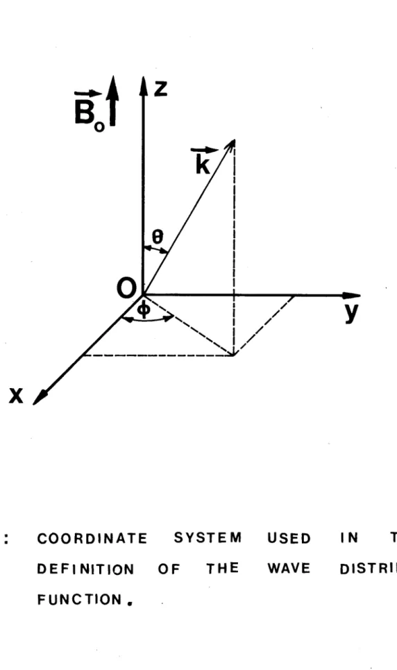
an azimuthal angle � (fig. 1) the angle 0 varies from 0 to 7r , and � from ° to 2 ir . In this représentation, the distribution function will be written
F ( u), 6 , 4� and the élément of wave energy is F (�d,6 ,$) d3r d w d9" d-f� The relation between this and the previous form of the distribution function is
(1.1.) F (w, 6. *) " Vg" k sin e F (k)
where k = j k| and V7
=
1 (d w / 9 ) e| is th modulus of the group velocity (BEKEFI, 1866) the vector
has the direction of the wave normal (or the opposite
direction, if (9�o/3Mfl is négative), as distinct from the group-ray velocity which has the direction of the géométrie
optics ray (HELLIWELL, 1965).
The représentation of the distribution function
for an electromagnetic wave mode in a magnetoplasma in terms of the variables to, 6, and� is analogous to that for a charged particle species, in the présence of a magnetic field, in terms of the energy E and the pitch-angle a . There is the différence that, for low-energy particles, the
distribution function has cylindrical symmetry around the
magnetic field, so no azimuthel angle is required, whereas
for waves, although most known source processes give rise to
distributions having such symmetry. this is lost progressively
by refraction as the waves are propagated away from their source
région. Incidentally, it should he remembered that the.
distribution functions of the energetic charged particles
in the earth's radiation belts are not cylindrically
symmetrical at énergies such that the radii of gyration are
comparable with the linear scale of the gradients of the
magnetic field (i.e. with an earth radius) or with the
atmospheric scale height in thR case of particles trapped
on low L - shells (HESS. 1968).
There is one respect in which the représentation
F (u . 8, �) of the wave distribution function is actually better than the représentation F (k) : namely, it is
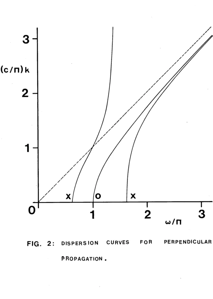
unambiguous. For e lectromagnet ic waves in a given mode. propagated in a given direction, it is possible for a given value of k to correspond to two (or more) différent values of w . This point is illustrated in fig. 2, which shows
the real branches of the dispersion curves for waves propa-
gated psrpendicu larly to the magnetic field ( 6 = tt/2) j � the électron gyrofrequency has been taken equal to tha
plasma frequency. The abscissa is w / II , where n is the
- 9 -
where c is the speed of light in free space i the dashed
line is the free-space dispersion curve to ck. Note that
the function w (k) is ambiguous for the extraordinary (X)
mode, though not for the ordinary (0), whereas the function
k ( to) is single-valued for hoth modes. In gênerai, for a given mode, a given value of w always corresponds to a unique value of k, and for this reason the représentation
F ( w, 0, �) is to be preferred.
Another reason is that the expérimenter, b� means of narrow-band filters, can sélect for observation waves
with frequencies w that lie between limits of his choosing.
Of course, the observed frequencies are equal to the true
wave frequencies only if the point of observation is
stationary with respect to the médium, because any motion
gives rise to Doppler shifts- proport ion al to k j hère this
has been assumed to be the case (see appendix A.). From this
point onwards, therefore, the distribution function for wave
energy will be used exclusively in the représentation
F (w, 6 ,$) .
In conclusion of this section, and in anticipation of
those that follow, it should be stated that the term "energy"
is employed in this paper in two différent sensés. In the
context of wave propagation theory, it is used in its strict
and customary sensé as above. However, when discussing the
analysis of data on the six field components, we shall use
it also in the sensé of signal theory, where for instance
if x(t) and y (t) are two real time séries, then
o x (t) dt and 10 y (t) dt are their respective énergies
in the time interval 0 � t � T while / x (t) y (t)dt is their interaction energy. We shall distinguish between thèse
two sensés, by using the terms "wave energy" and "signal
energy" respectively ; equally we shall speak of "wave power"
- 10 -
3. STATISTICAL DESCRIPTION OF THE RECEIVED SIGNALS
3.1. Wide-band signais
When we seek to predict the statistics of the six
components of a random wave field, the first question to ask is how thèse statistics should be described. As already
mentioned, the field is pictured as being made up of a
continuum ofelementary plane waves of différent frequencies
and with random phases, propagated through the médium in
différent directions. We suppose that, at a fixed point in the médium, continuous measurements are made of three
orthogonal electric components and three orthogonal magnatic
components of the total field, using for instance three electric
dipole antennae and three maenatic loop antennae. For the
time being. we suppose that thèse mRasuraments are madR ov�r a wide frequency band. Wr take a right-handed set of rectangular coordinate axes Oxyz, with Oz parallel to the steady magnetic
field, and suppose for convenience that the antennae are
aligned parallel to thèse axes. Then the expérimental data
consist of six wide-band signais, each proportional to one
of the six axial field
components.
First let us consider the individual properties of
any one of thèse signais, separate from the other five. It
is the sum of ail the waveforms induced on the corresponding
antenna by ail the différent elementary plane waves. The
elementary wareform induced by any one of thèse waves is a
sinusoid, the phase of which bears no spécial relationship
to that of the sinusoid induced by any other such wave. Thus
the total signal is the sum of an infinité number of elementary
sinusoids, with infinitésimal amplitudes and random phases.
It is well known that a signal of this type is a stationary Gaussian random process of zéro mean value, and that, as such;
its statistical properties are described completely by its
mean auto-covariance function or hy its mean signal power
spectrum ("auto-spectrum").
As usual when discussing random processes, it is
We imagine an ensemble of random wave fields. each giving
rise to a spécimen of the random signal considered. We assume that, on �oing from one member to another of the ensemble of fields, the elementary plane waves change in
amplitude, frequency, direction of propagation, and phase,
while remaining consistent collectively with thR given wave
distribution function. On this assumption. the received signal
is ergodic, so its auto-corariance function and auto-spectrum
can be defined alte mat ive ly in terms of time averages or
of ensemble averages.
Now let us consider the six received signais as a
whole. Besides their individual properties, we need to know
what relationships exist between them. Thèse are described
by the cross-covariance functions for ail the fifteen possible
pairs of signais, or by the corresponding cross-spectra.
Hère we prefer to work with signal auto-spectra and
cross-spectra, rather than to use covariance functions, because
the spectra are related more simply to the wave distribution
function, as we shall show later 1 of course, we can get from
a covariance function to the corresponding power spectrum, or
vice versa, by a direct or inverse Fourier transform
respectively (JENKINS and WATTS, 1969).
First, let us define a 6 x 6 spectral matrix, which groups ail the statistical data together in a convenient way, Let Ex, Ey, Ez be the axial components of the electric field
of the wave at the point of observation, and
Hx , Hy, Hz the components of the wave magnetic field. From thèse variables,
we define a generalized electric field vector E as folio w s :
where
7 is the wave impédance of free space. (Note : another
way of defining a generalized electric field vector is mentioned in appendix B). This step in the argument is just a convenient way of regrouping the data, and has no physical
- 12 -
significance. Let Ei be any comportent of this vector, the
subscript i running from 1 to 6. We now introduce the
6 x 6 spectral matrix, of which any élément
Sij ( w) is either the auto-power spectrum of the field component f (if i = j), or the cross-power spectrum of the components ri and Ej
(if i / j) .
Thèse are "two-sided" signal power spectre : that is,
they hâve values at négative as well as at positive frequencies.
They are the Fourier transforms of the corresponding covariance
functions. Since the latter functions are purely real, it
follows that
Sij ( w) - sfj w), where the asterisk
dénotes the complex conjugate 1 therefore it suffices to quote
the expressions for the spectra at positive frequencies only.
At any one frequency w,the spectral matrix contains
36 items of statistical information about the field. It
might be thought that the number of indépendant items is less
than this, because the matrix is Hermitian : Sij ( to ) » Sjï (to Hence hère are only 6 independent auto-spectra and 15
cross-spectra. Note. howevnr, that while the auto-spectra
are purely real, since the auto-covariance functions are
symmetrical, the cross-spectra are complex, since the cross-
covariance functions are asymmetrical in gênerai. Moreover
the real and imaginary parts of the cross-spectra are mutually
independent, i.e. there is no gênerai relation between them.
Hence the numher of indépendant items of information is 36
as stated.
3.2. Narrow-band sienals
Now let us consider tho case where the 6 data signais are received in a band of width 6w centred on some frequency
wo. We suppose moreover that this band is narrow, by
which we mean two things : firstly, that Ato
��u� 1 secondly, that ail the 36 signal power spectra Si., ( w) are essentially
constant and equal to
- 13 -
Then clearly the information contained in the received signais
relates only to the values of the 36 ouantities
S.. ( w Q ) j 3 the question is how to extract the relevant information from
the data.
Let
Xi (t) be the real narrow-band signal obtained by
filtering the original wide-band signal Ei (t) through the
receiver pass-band. Let X i (t) be the corresponding analytic
signal, i.e. the représentation of Xi (t) by a complex exponential (HELLSTROM, 1968). We now define the covariance
matrix {cij } of the set of 6 narrow-band real signais, with (1.3) Cij - � X i (t)
Xj* (t) �
where the triangular brackets dénote the (BORN and WOLF, 1964)
ensemble average or "expected value" of the product. If the
signais are stationary and ergodic, as has been assumed, then
thèse same quantities are given by the corresponding time
averages in the limit of very long times. A practical method for estimating the éléments
c..
of the covariance matrix
in this way has been described bv MEANS (1972).
In order to relate thèse éléments to those of the spectral
matrix at the frequency
u . it is necessary to define the bandwidth Au more precisely. If the transfer function of the
receiver is Y (00 ), between the point where the signal
E i (t) enters it and that at which Xi (t) émerges, and if, at positive frequencies, this function takes the form of a
single peak with its summit at w
o , then
we define
In engineering parlance, this quantity is known as the
noise bandwidth (BENDAT and PIERSOL, 1971).
With Au thus defined, it follows from elementary
considérations of signal energy conservation that
2 (1.5)
Cij
= 4 Au
ly Cw0) 1 Sjj (wo)
The factor 4 stems from the fact that, at positive frequencies, the amplitudes of the Fourier components of x i (t) are twice those of the corresponding components of Xi (t).
- 14 -
4. DIRECT RELATIONSHIP BETWEEN WAVE AND SIGNAL STATISTICS
The problem is to relate the spectral matrix, which
describes the statistics of the 6 received signais, to the
distribution function, which describes those of the random
wave field. In order to do this, we shall show how each of
thèse entities is made up of contributions from ail the
various elementary waves we begin with the case where
thèse waves ail belong to the same magneto-ionic mode.
First let us consider one such wave, which we shall
distinguish from its fellows by placing the subscript 1 in
front of every symbol that refers to it. The i'th component
of its generalized electric field, which will be called
le:i (t, t), varies sinusoidally as a function of time and of spatial position :
On the right-hand side of this eouation, the symbol Re dénotes
the extraction of the real part, lei is the complex amplitude,
the angular frequency lW is real and positive, and the
wave-number vector lk is real because the médium is assumed to
be lossless, and also because only homogeneous waves are
being considered, as befits a situation in which there are no boundaries.
Now if, in coordinate space, the wave has an electro-
magnetic energy density IP. thpn its distribution function,
which we shall call if (k), is a 3-dimensional Dirac
distribution of strength
pat the point lk in k space : (1.7)
If (it)
»
ip 6(k - :it)
The alternative form of this distribution function is
(1.8)
if ( u),
6.4
�
) =
ip
�
5(oi -
iw ) 6(6 - 10
6(4.-^
where le and l� are the angles that specify the directionof ik. The équivalence of thèse two expressions is évident, because in both cases the wave enerey per unit volume of
coordinate space is given by a triple intégral over the distribution function :
- 15 -
In spite of superficial appearances, the expressions (1.7)
and (1.8) are consistent with (1.1) j the algebraic factors
on the right-hand side of (1.1) are incorporated in the
delta-functions on the right-hand side of (1.8).
The éléments of the spectral matrix for this same
elementary wave are, for u positive,
Probably the simplest way to dérive this resuit is to obtain
the expression for the cross-covariance function of the
periodic signais ici
(t) and
,ej (t) at a fixed point r, and then to take its Fourier transform.
Now. instead of considering just one elementary wave,
let us consider the subset of elementary waves fer which the
parameters jw, 10. and 14 lie respectively in the ranges
from m to 00 + dw , from 6 to 6 + dO . and from � to d� Their contribution to the wave energy per unit volume of
coordinate space is E
lp , where the sun ia taken over
this subset. Bv définition, the distribution function for
the random field is related to this quantity as follows :
(1.11) F ( u, 6, +) dw d6 d, � ip � 1
Hère the brackets on the right-hand side dénote the ensemble
average.
Similarly, the elementary waves in this subset make
the following contribution to the signal energy of interaction
between the field components Ei and Ej , in the frequency
range from w to 00 + d w :
At this point we introduce a crucial idea : for given
values of u , 9 . and �. the wave energy density p is propor-
tional to the square of the amplitude of any one field component i
the same is true of the product lei le j therefore the
- 16 -
is independent of the amplitude, and is essentially the
same for ail the elementary waves in the subset defined
above, i.e. it is independent of 1. With ail the possible
pairs of values of the indices i and j, the identity
(1.13) defines 36 such ratios. The expressions for them,
as functions of w, 9 , and � and of the characteristic parameters of the plasma, are given by the propagation
theory for the type of wave considered, i.e. by the
magneto-ionic theory in the présent instance 1 they are quûted in the appendix B. It is at this point that our
knowledge of the properties of the médium enters into the
argument.
This idea enables us to write
with (1.15) following from (1.11), and enabling us to cancel
du on both sides.
Finally, in order to obtain the total auto-spectral
(i » j) or cross-spectral ( 1 0 J) signal energy in the frequency range from w to w + du it suffices to sum over the complète set of elementary waves in this range, with ail
possible directions of propagat ion . in other words, (1.15)
must be integrated over the full ranges of the angles 8 and Then, dividing by du we obtain
(1.16) S i j
( u) =
-y- ; o
J ai j
C u.
F ( w.
6,
�
)
d
6 d
for w positive. This is the required resuit, for the spécial case where only one of the two magneto-ionic modes areprésent.
In the general case where both modes are présent simultaneously, each spectral matrix élément is just the sum of the contributions from the two modes :
- 17 -
where the subscript m dénotes the wave mode.
From their définitions, it follows that the spectral
matrix
S ^ j together with the kernels aii for the two modes,
- 18 -
5. CONLUSION
Subject to the assumptions made in this paper. équation
(1.17) is the solution for the direct problem of determining the
statistics of the received signais when those of the wave
field are known.
As such, it already provides a weak basis for
comparison between theory and experiment in the study of the
origin of certain natural random Rlectromagnetic wave fields,
such as those of magnetospheric VLF and ELF hiss. If the
theory predicts the wave distribution function explicitly,
and if an accurate estimate of the spectral matrix is available
from expérimental data, then the two can be compared by means
of this equation.
More often, however, the task of comparing theory and
experiment is less simple. Tha data may be degraded by noise,
or the time of observation too short to yield good statistics.
The theory may involve one or more unknown parameters, which
hâve to be adjusted in order to make its prédictions agrée
with the data as closely as possible. There may be several
competing théories, none of which explains the data perfectly,
and then one wants to know whether any of thèse théories is
acceptable, and if so, which is the most plausible. Or again,
one may be interested in analyzing some expérimental data to
find out whatever one can about the wave distribution function.
in the absence of any theoretical model. Ail there are différent
forms of the inverse problem, which is more difficult and
will be treated in subséquent papers.
At the same time, further work is needed on the direct
problem, in order to free the theory from the limitations
accepted in this paper. For instance, before it can be applied to space-probe data on the random field of Alfven waves in the
solar wind, the theory must be generalized to take account
of the motion of the point of observation with respect to
the médium, and to make use of data on the wave-induced
fluctuations of plasma velocity. The application to random
wave fields other than electromagnetic must be considered.
has been noted already, in section 2. Another interesting
special case is that in which the wave field is random in
space but not in time, an example being the field created
when an initially plane monochromatic wave traverses a
spatially irregular but temporally stationary médium. The
study of this case would begin to forge the links between two
domains hitherto independent, namely previous work on the
propagation of deterministic wave fields through random média,
and the présent work on the analysis of measurements of rendom
wave fields in uniform média.
ACKNOWLEDGEMEIMTS
The authors are most grateful to Professor D.A.'Gurnett
for suggesting this problem, in a private communication to L.R.O. Storey in 1965. The work was begun in 1972 when one
of us (L.R.O.S) was a guest worker at the Institute for Extraterrestrial Physics of the Max-Planck Institute for
Physics and Astrophysics, Garching (German Fédéral Republic),
at the kind invitation of Dr. G. Haerendel. Our thanks are
- 20 -
REFERENCES
BEKEFI, G. "Radiation Processes in Plasmas",
Wiley, New York, 1966.
BENDAT, J.S. and A.G. PIERSOL, "Random Data :
Analysis and Measurement Procédures".
Wiley, New York, 1971.
BORN, M. and E. WOLF, "Principles of Optics" (4th. ad.),
Pergamon, London, 1970.
BUDDEN, K.G. "Radio Waves in the Ionosphère",
University Press, Cambridge (G.B.) 1961.
GRARD, R. "Interprétation de mesures de champ électromagnétique
T.B.F, dans la maznAtosohAre",
Ann. Géophys. 24, 955-971, 1968.
HELLIWELL. R.A. "Whistlers and related
Ionospheric
Phenomena". Stanford University Press.
Stanford. 1965.
HELLSTROM. C.W. "Statistical Theory of Signal Détection"
(2 nd.ed.). Pergamon London,1968.
HESS. W.N. "The Radiation BRlt and the MaEnetosphere".
Blaisdell. Toronto, 196R.
JENKINS. G. M. and D.G. WATTS. "Spectral Analysis and its
Applications". Holdan-Day, San Francisco. 1969.
LYONS. L.R., THORNE. R.M. and C.F. KENNEL. "Pitch-angle
diffusinn of radiation-belt électrons within
the plasmasphere", J. Geophys. Res. 77
- 21 -
MEANS. J.D. "The use of the three-dimensinnal covariance
matrix in analyzing the polarization properties
of plane waves". J. Geophys.
Res. 77. 5551 - 5559, 1972.
riHZER. F.S. "Analysis of techniques for measuring ne and AC
electric fields in thp magnetosphere". Space
Sci. Rev. 14. 272-�13 1973.
RATCLIFFE. J.A. "The Magneto-ionic Theory and its Applications
to the Ionosphère". University Press,
Cambride (G.B.). 1959.
RUSSELL. C.T. Mc. PHERRON, R.L., and P.J. COLEMAN,
"Fluctuatine magnetic fields in the magnetosphere :
1- ELF and VLF fluctuations". Space Sci.
Rev. 12. 810-856, 1972.
SCHULZ. M. and L.J. LANZEROTTI. "Particle Diffusion in the
Radiation Belts". Springer-Verlas, Berlin. 1P7'".
SHAWHAN. S.D. "The use of multiple receivers to measura
the wave characteristics of very-low-f reouency
noise in space". Space Sci. Rev. 10, 639-736. 1°?-.
STOREY. L.R.O. "A method for measuring local électron density from an artificial satellite". J. Re;;. Nat. Bur.
Stand. 63 D. 325-340, 1959.
STOREY. L.R.O. "Electric field experiments : - alternating
fields", in "The ESRO geostationary magnetospheric
satellite". European Space Research Organisation,
Neuilly-sur-Seine, Report n° SP-60, 267-279, 1971.
STOREY. L.R.O. and F. LEFEUVRE, "Theory for the in terpret at ic-
of measurements of a random e lect romagnet ic wave field in space". in "Space Research XIV" (Eds :
M ..1 . RYCROFT and'R.D. REASENBERG ) Ak ademie-Vc r lag ,
- 22 -
THORNE. R.M.. SMITH. E.J. , BURTON. R.K. and R.E. HOLZER.
"Plasmaspheric hiss". J. Ceophys. Res. 78. 1581-
- 23 -
APPENDIX A : Validity of the basic concepts and assumrtions.
In section 2, it is assumed that the random wave fielri
is statistically stationary in space and in time, and that
only one wave mode is présent. Thèse assumptions are less
restrictive than mipht appeau at first si�ht. The conditions undar which they may be considered to be satisfied adequately
are discussed bslow,
Approximate spatial uniformity is required only to
ensure that thR structure of a single wave be very littlp différent from what it would be in an infinité uniform
médium, with properties like those of the real medium at
the point considered. For this purpose, it is necessary that
the médium be uniform on a scale much larger than a wavalength. The residual large-scale non-uniformity limits the meaningful
détail that the distribution function can exhibit : if L is the distance over which the médium is substantially uniform,
then this functinn can he specified with a résolution, in any
component of k, of the order of Ak = 2* /L.
Aporoximate temporal stationarity of the field is
needed to provide reasonable data statistics, which means
that the received signais must be statistically stationary
over time intervais much longer than a wave oeriod. If they
are in fact so for a time T, than the distribution function
can he measured with a resolution in frequency of the order
of Au = 2 ir/T (moreover, the point of observation is effectively stationary if ail Doppler shifts due to its
motion are less than Au ) .
Under the conditions enunciated in the previous two
paragraphs, it is possible to define a wave distrihution
function that varies with time t and with spatial position
r , as was mentioned in section 2. For this purpose, the
fields must he truncated hy means of a suitable "window"
function, of linear dimensions L and duration T, centred
on the point-instant (r, t) considered, before taking
their Fourier transforms i the choice of L and T also limits
the meaningful resolution of F in wave number and in frequency respectively.
- 24 -
Thèse same conditions justify the use of géométrie
optics to détermine how a given distribution function evolves in tine and in space (BEKEFI, 1966), In the présent paper,
such questions hâve been avoided by the assumption of
stationarity.
Finally, the assumption that only one wave mode is
présent is satisfied over wide frequency ranges, in particular in the range from the lower hy brlri f requen cy up to the
électron gyro-frequencyoinwhichonly the whistler (ordinary)
mode is propagated. Even at frequencies where both modes can
be propagated, natural source mechanisms are likely to excite
one much more strongly than the other. Finally, as we saw
in section 4, this assumption can be dropped if necessar� without greatly complicating the theory.
- 25 -
APPENDIX B : expressions for the kernels
aij and bij The 36 functions
ai1 (u,8,�J�), which are the kernels of the set of intégral équations (1.16), were defined by
(1.13) in the course of an analysis based on a right-handed rectangular coordinate System Oxyz, with Oz parallel to the
steady magnetic field. For pratical purposes, algebraic
expressions are required for thèse weighting functions in
terms of the variables w, Oand and of the characteristic
parameters of the médium.
However, since the médium has been assumed to be
uniaxial, the required expressions would hâve been simpler
if the analysis had been developed using a "circularly- polarized" coordinate system (STIX, 1962), in which the
complex amplitudes of the sinusoïdal components of the
electric field vector e of an elementary plane wave are
(1.18)
eR mex iey eL::I ex - iey ap
ez
and similarly for the magnetic vector h. The subscripts
R, L, and P stand for "right-handed", "left-handed", and "parallel" respectively. We now define a generalized electric field vector f, the 6 components of which hâve the complex amplitudes
Then, redeveloping the analysis along the lines of
section 4, we are led to define a new set of 36 kernels,
for which we shall now quote the expressions.
First. hnwever, we must define thn plasma parameters..
In this we shall follow STIX (1962). with some minor
différences : in particular. we suppose that the plasma
containsonly électrons and positive ions, and that the
latter, of which there may be several species oresent, are
ail singly charged. Denoting thn different types of chareed
particle - including the électrons - by a subscriot k, let
- 26 -
per particle, and q the charge per narticle. For eech type
of particle, we now define two charactRristic fmaufincies :
the an�ular plasma frenuencv IIk, such that
where en is the electric
permit tivity of free space. and
the aneular gyrof reauancy
where 80 is the magnitude of the induction vector of tha
steady magnetic field. The minus sien has heen put into this
définition so as to �ive
fik the sien of the natural sensé of
gyration of the particles around the field (e.g. positive
for the électrons, which gyrate in a right-handed sensé). Lastly. we define three dimensionless quantities :
Thèse auantitias arR identical with those that Stix dénotes
by the same symhols i in the expressions that follow , they
represent thp oroperties of the plasma.
From thèse wr must define several derived
quantifies,
the first of which is the phase refractivn index n for
e lect romagnet ic waves in either of the two magneto-ionic modes. This Quantité is the solution of the équation
which is a
- 27 -
For a given 0 and given plasma paramRters. (1.24) may hâve two, one.,, or no roots with n positive. Only such positive roots, which correspond to freely propagated modes, are to
be considered here 1 négative roots correspond to evanescent modes. Moreover. for a given positive n , only the positive value of n will be considered, the négative value corresponding
to a wave propagated in the opposite direction. On the
questions of the nomenclature for the two modes, and of their
correspondence with the roots, the reader should consult the
standard works on the magneto-ionic theory (RATCLIFFE 1959,
BUDDEN 1961).
One more dimensionless quantity remains to be defined.
It involves the group refractive index
and two other parameters :
In thèse t�rms� the required quantity is
We are now in a position to list the 36 kernels
b^ , . In
point of fact� it sufficns to list the 6 kernels with i-j, and 15 kernels with i/j, since the rnmaining 15 are given by
the relation
bJi - =
b"^, which follows from
their de-Finition
- 29 -
The dérivation of thèse results. which is s traightf orward
but lengthy, will bR
published elsewhere. They apply to
both magneto-ionic modes 1 however, thn values of n and ofÇ are différent for the two modes, so in general the
bij are
différent also.
Thèse kernels can be used directly for interpreting
data on random wave fields, provided that the 6 field components are transformed to the circularly-polarized coordinate System
bafore being used to estimate their spectral matrix. On the
other hand. if one prefers to work with data in the rectangular
System Oxyz, then one req.uires the kernels
a...
which are
given in terms of the bij by the following expressions :
The 3 other kernels with i and ^3 can he found by using the relation a.. = a From this set of 9 kernels, the remaining 27 with i and/or j) can be obtained by adding 3 to the first and/or second subscript of every term in each
expression. Thèse results follow quite simply from the