HAL Id: inria-00387749
https://hal.inria.fr/inria-00387749
Submitted on 2 Jun 2009
HAL is a multi-disciplinary open access
archive for the deposit and dissemination of
sci-entific research documents, whether they are
pub-lished or not. The documents may come from
teaching and research institutions in France or
abroad, or from public or private research centers.
L’archive ouverte pluridisciplinaire HAL, est
destinée au dépôt et à la diffusion de documents
scientifiques de niveau recherche, publiés ou non,
émanant des établissements d’enseignement et de
recherche français ou étrangers, des laboratoires
publics ou privés.
Register allocation by graph coloring under full
live-range splitting
Sandrine Blazy, Benoît Robillard
To cite this version:
Sandrine Blazy, Benoît Robillard. Register allocation by graph coloring under full live-range splitting.
ACM SIGPLAN/SIGBED Conference on Languages, Compilers, and Tools for Embedded systems
(LCTES’2009), ACM, Jun 2009, Dublin, Ireland. �inria-00387749�
Live-Range Unsplitting for Faster Optimal Coalescing
Sandrine Blazy
Benoit Robillard
ENSIIE, CEDRIC {blazy,robillard}@ensiie.fr
Abstract
Register allocation is often a two-phase approach: spilling of regis-ters to memory, followed by coalescing of regisregis-ters. Extreme live-range splitting (i.e. live-live-range splitting after each statement) en-ables optimal solutions based on ILP, for both spilling and coa-lescing. However, while the solutions are easily found for spilling, for coalescing they are more elusive. This difficulty stems from the huge size of interference graphs resulting from live-range splitting. This paper focuses on coalescing in the context of extreme live-range splitting. It presents some theoretical properties that give rise to an algorithm for reducing interference graphs. This reduction consists mainly in finding and removing useless splitting points. It is followed by a graph decomposition based on clique separators. The reduction and decomposition are general enough, so that any coalescing algorithm can be applied afterwards.
Our strategy for reducing and decomposing interference graphs preserves the optimality of coalescing. When used together with an optimal coalescing algorithm (e.g. ILP), optimal solutions are much more easily found. The strategy has been tested on a standard benchmark, the optimal coalescing challenge. For this benchmark, the cutting-plane algorithm for optimal coalescing (the only opti-mal algorithm for coalescing) runs 300 times faster when combined with our strategy. Moreover, we provide all the optimal solutions of the optimal coalescing challenge, including the three instances that were previously unsolved.
Categories and Subject Descriptors D.3.4 [Programming lan-guages]: Processors - compilers, optimization; G.2.2 [Graph the-ory]: Graph algorithms
General Terms algorithms, languages
Keywords register allocation, coalescing, graph reduction
1.
Introduction
Register allocation determines at compile time where each variable will be stored at execution time: either in a register or in memory. Register allocation is often a two-phase approach: spilling of reg-isters to memory, followed by coalescing of regreg-isters [3, 8, 16, 5]. Spilling generates loads and stores for live variables1 that cannot 1A variable that may be potentially read before its next write is called a live
variable.
Permission to make digital or hard copies of all or part of this work for personal or classroom use is granted without fee provided that copies are not made or distributed for profit or commercial advantage and that copies bear this notice and the full citation on the first page. To copy otherwise, to republish, to post on servers or to redistribute to lists, requires prior specific permission and/or a fee.
LCTES’09, June 19–20, 2009, Dublin, Ireland.
Copyright c 2009 ACM 978-1-60558-356-3/09/06. . . $5.00.
be stored in registers. Coalescing allocates unspilled variables to registers in a way that leaves as few as possible move statements (i.e. register copies). Both spilling and coalescing are known to be NP-complete [24, 6].
Classically, register allocation is modeled as a graph coloring problem, where each register is represented by a color, and each variable is represented by a vertex in an interference graph. Given a number k of available registers, register allocation consists in finding (if any) a k-coloring of the interference graph. When there is no k-coloring, some variables are spilled to memory. When there is a k-coloring, coalescing consists in choosing a k-coloring that removes most of the move statements.
ILP-based approaches have been applied to register allocation in order to provide optimal solutions. Register allocation is one of the most important passes of a compiler. A compiler performing an optimal register allocation can thus generate efficient code. Having such a code is often of primary concern for embedded software, even if the price to pay is to use an external ILP-solver. Appel and George formulate spilling as an integer linear program (ILP) and provide optimal and efficient solutions [3]. Their process to find optimal solutions for spilling requires live-range splitting, an opti-mization that leaves more flexibility to the register allocation (i.e. avoids to spill a variable everywhere). While the solutions are easily found for spilling in this context, for coalescing they are more elu-sive. Indeed, live-range splitting generates huge interference graphs (due to many move statements) that make the coalescing harder to solve.
Splitting the live-range of a variable v consists in renaming v to different variables having shorter live-ranges than v and adding move statements connecting the variables originating from v. Re-cent spilling heuristics benefit from live-range splitting: when a variable is spilled because it has a long live-range, splitting this live-range into smaller pieces may avoid to spill v. If the live-range of v is short, it is easier to store v in a register, as the register needs to hold the value of v only during the live-range of v.
There exists several ways of splitting live-ranges (e.g. region spilling, zero cost range splitting, load/store range analysis) [10, 7, 18, 19, 4, 11, 20]. Splitting live-ranges often reduces the interfer-ences with other live-ranges. Thus, most of the splitting heuristics have been successful in improving the spilling phase. The differ-ences between these heuristics stem from the number of splitting points (i.e. program points where live-ranges are split) as well as the sizes of the split live-ranges. These heuristics are sometimes difficult to implement.
The most aggressive live-range splitting is extreme live-range splitting, where live-ranges are split after each statement. Its main advantage is the accuracy of the generated interference graph. In-deed, a variable is spilled only at the program points where there is no available register for that variable. As in a SSA form, each vari-able is defined only once. Furthermore, contrary to other splitting heuristics, extreme live-range splitting is easy to implement.
Extreme live-range splitting helps in finding optimal and ef-ficient solutions for spilling [3]. However, it generates programs with huge interference graphs. Each renaming of a variable v to v1results in adding a vertex in the interference graph for v1 and,
consequently, some edges incident to that vertex. Thus, interfer-ence graphs become so huge that coalescing heuristics often fail. The need for a better algorithm for the optimal coalescing problem gave rise to a benchmark of interference graphs called the optimal coalescing challenge (written OCC in the sequel of this paper) [2]. Recently, Grund and Hack have formulated coalescing as an ILP [16]. They introduce a cutting-plane algorithm that reduces the search space (i.e. the space of potential solutions). Thus, their ILP formulation needs less time to compute optimal solutions. As a result, they provide the first optimal and efficient solutions of the OCC. These solutions are 50% better than the solutions computed by the best coalescing heuristics.
Grund and Hack conclude in [16] that their cutting-plane al-gorithm fails when applied to the largest graphs of the OCC. Be-cause of extreme live-range splitting (that was required for opti-mal spilling), optiopti-mal solutions for coalescing cannot be efficiently computed on these graphs. Owing to the extreme amount of copies, coalescing is hard to solve optimally. In this paper, we study the impact of extreme live-range splitting on coalescing and provide a strategy for reducing interference graphs before coalescing. ILP is commonly composed with algorithms in order to let the solver, that uses an exponential algorithm, only deal with the core of the problem. The work we present follows this classical methodology. Our strategy performs mainly two steps. The first step is the main step of the strategy and we call this step live-range unsplitting; it identifies most of the splitting points that are not useful for co-alescing, and updates the graph consequently. Then, a second step finds clique separators in the updated graph and thus decomposes it into several subgraphs. Coalescing on each subgraph is then solved separately. As the subgraphs are much smaller than the original graph, ILP solutions are much easier and faster to find. Moreover, both steps do not break the optimality of coalescing.
The remainder of this paper is organized as follows. Section 2 recalls some definitions form graph theory and defines some terms that are computed by our strategy for optimal coalescing (e.g. split interference graphs, that are the interference graphs resulting from extreme live-range splitting). Section 3 presents the main contri-bution of this paper. It details our algorithm for live-range unsplit-ting, that reduces split interference graphs. Then, section 4 defines our whole strategy for optimal coalescing. This strategy performs mainly live-range unsplitting and then a graph decomposition.
Section 5 presents experimental results on the OCC. A first re-sult is that our live-range unsplitting reduces the size of original graphs (i.e. before extreme live-range splitting) by a factor of up to 10, and thus extreme live-range splitting does not make coalescing harder anymore. A second result is that Grund and Hack’s cutting-plane algorithm for optimal coalescing runs 300 times faster when combined with our strategy, thus enabling to solve all the instances of the OCC, including the 3 instances that were previously un-solved. Related work is discussed in Section 6, followed by con-cluding remarks in Section 7.
2.
Foundation
This section defines split interference graphs and SB-cliques, as well as some concepts from graph theory.
Register allocation is performed on an interference graph. There are two kinds of edges in an interference graph: interference (or conflict) edges and affinity (or preference) edges. Two variables in-terfereif there exists a program point where one variable is live at the exit of a statement that defines the other variable (and the state-ment differs from a move statestate-ment between both variables) [1].
An affinity edge between two variables represents a move statement between these variables (that should be stored in a same register or at the same memory location). Weights are associated to affinity edges, taking into account the frequency of execution of the move statements.
Given a number k of registers, register allocation consists in satisfying all interference edges as well as maximizing the sum of weights of affinity edges such that the same color is assigned to both endpoints. Satisfying most of the affinity edges is the goal of register coalescing.
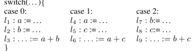
Interference graphs are built after a liveness analysis [9]. In an interference graph, a variable is described by a unique live-range. Consequently, spilling a variable means spilling it everywhere in the program, even if it could have been spilled on a shorter live-range. Figure 1 illustrates this problem on a small program consist-ing of a switch statement with 3 branches (see [21] for more de-tails). The program has 3 variables but only 2 variables are updated in each branch of the switch statement. Thus, its corresponding interference graph is a 3-clique, that is not 2-colorable, although only 2 registers are needed.
switch(. . . ){
case 0: case 1: case 2:
l1: a := . . . l4 : a := . . . l7: b:= . . .
l2: b := . . . l5 : c := . . . l8: c:= . . .
l3: . . . := a + b l6 : . . . := a + c l9: . . . := b + c
}
Figure 1. Excerpt of a small program such that its interference graph is a 3-clique.
The usual way to overcome the previous problem is to perform live-range splitting. Extreme live-range splitting splits live-ranges after each statement, and thus generates some renamings that are not useful for coalescing. When v is renamed to v1and v2, if after
optimal coalescing v1and v2share a same color, then the renaming
of v2 is useless: v2 can be replaced by v1 while preserving the
optimality of coalescing.
Moreover, the number of affinity edges blows up during extreme live-range splitting since there is an affinity edge between any two vertices that represent the same variable in two consecutive statements. Figure 2 shows the split interference graph of a small program given in [1]. In the initial interference graph, each vertex represents a variable of the initial program (the array mem is stored in memory); the affinity edges correspond to both assignments d:=c and j:=b.
The bottom of Figure 2 is the split interference graph resulting from extreme live-range splitting on the graph at the top of the Fig-ure. The construction of the split interference graph is inspired from the construction of the OCC by Appel and George. Every variable vithat is live-in and live-out2at program point p is renamed into
vi+1at this program point (i.e. the variables are renamed in parallel
with the statement of p). For instance, k0, k1 and k2 are copies of k. As k is live initially, it is renamed (at program point p0) to k0
(and so is j). Similarly, g and j0 are renamed to respectively g0 and j1 at program point p1, but the variable k is not renamed, as
it dies (i.e. it is not live-out) at p1. In order to show how the edges
of the first graph (on the top of the figure) are transformed into the edges of the second graph (bottom of the figure), the edges(j, k) and(j, b) of the first graph and their corresponding edges in the second graph are bold edges. The renamings are done in parallel in order to limit the interferences between the newly created
vari-2Given a program point p, a variable is live-in (resp. live-out) if it is live
Live-in : k j (p0) g := mem[j+12] (p1) h := k - 1 (p2) f := g * h (p3) e := mem[j+8] (p4) m := mem[j+16] (p5) b := mem[f] (p6) c := e + 8 (p7) d := c (p8) k := m + 4 (p9) j := b (p10) Live-out : d k d e g h k m j b Live-in : k j (p0) k0 := kk j0 := j k g := mem[j+12] (p1) j1 := j0k g0 := g k h := k0 - 1 (p2) j2 := j1k f := g0 * h (p3) f0 := fk j3 := j2 k e := mem[j2+8] (p4) e0 := ek f1 := f0 k m:=mem[j3+16] (p5) e1 := e0k m0 := m k b:=mem[f1] (p6) b0 := bk m1 := m0 k c := e1 + 8 (p7) b1 := b0k m2 := m1 k d := c (p8) b2 := b1k d0 := d k k1 := m2 + 4 (p9) d1 := d0k k2 := k1 k j4 := b2 (p10) Live-out : d1 k2 k j k0 j0 g g0 h j1 f j2 e f0 j3 e0 f1 m m0 b e1 m1 b0 m2 b1 d k1 b2 d0 k2 j4 d1 (p0) (p1) (p2) (p3) (p4) (p5) (p 6 ) (p 7 ) (p 8 ) (p 9 ) (p 10 )
Figure 2. A small program and its interference graph (top). Full edges are interference edges. Affinity edges are dashed edges. The same program after extreme live-range splitting and its split interference graph (bottom). The weights of affinity edges are omitted in the Figure. The program points(p0) . . . (p10) of both programs are shown in the Figure.
ables and the other variables. For instance, in the first statement (at program point p0), k0 interferes with j0 but not with j.
Edges corresponding to renamings are added in the split inter-ference graph. Affinity edges between renamed variables are also added, as well as interference edges related to renamed variables. For instance, renaming j to j0 generates the affinity edge (j, j0). More precisely, an interference edge(x, y) in the initial graph gen-erates (in the split interference graph) n interference edges between a renaming x′
of x (or x itself) and a renaming y′
of y (or y it-self), where n is the number of program points where x and y in-terfere in the initial program. For instance, the inin-terference edge (j, k) (of the initial graph) corresponds to the three interference edges(j, k), (j0, k0) and (j4, k2) of the split interference graph, because in the initial program, j and k interfere at program points p0, p1and p10. Similarly, the affinity edge(j, b) of the initial graph
corresponds to the affinity edge(j4, b2) of the split interference graph, and this is the only affinity edge originating from(j, b) as there is only one move statement j:=b in the initial program.
The main drawback of extreme live-range splitting is that it generates huge graphs. There are two kinds of affinity edges in a split interference graph: edges representing coalescing behaviors, and edges added by variable renaming during live-range splitting.
A lot of affinity edges and vertices (as well as some associated edges) corresponding to variable renaming are added in the graph. This section gives two properties of these edges and vertices that are useful for reducing the graphs.
Clique. A clique of a graph G is a subgraph of G having an edge between every pair of vertices. A clique is said to be maximal if there is no other clique containing it.
Interference connected component. Given a graph, an interfer-ence connected componentis a maximal set of vertices such that there exists a path (of interference edges) between any pair of its vertices.
Interference clique. An interference clique is a clique containing only interference edges. For instance, the subgraph induced by the vertices b0, c and m1 is an interference clique that we call C. The subgraph induced by the vertices b1, d and m2 is also an interference clique that we callC′
.
Theorem 1. After extreme live-range splitting, a statement corre-sponds to an interference connected component of the split interfer-ence graph. Moreover, such a component is an interferinterfer-ence clique, that we call a statement clique.
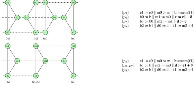
m0 b e1 b01 m12 cd k1 b2 d0 m0 b e1 m1 b0 c m2 b1 d k1 b2 d0 (p8) (p9) (p7) (p6) (p9) (p7,p8) (p6) (p5) e1 := e0k m0 := m k b:=mem[f1] (p6) b0 := bk m1 := m0 k c := e1 + 8 (p7) b1 := b0k m2 := m1 k d := c (p8) b2 := b1k d0 := d k k1 := m2 + 4 (p5) e1 := e0k m0 := m k b:=mem[f1] (p6, p7) b1 := bk m2 := m0 k d := e1 + 8 (p8) b2 := b1k d0 := d k k1 := m2 + 4
Figure 3. Some parallel cliques and the corresponding piece of code (top). The same subgraph (and the corresponding piece of code) after our graph reduction (bottom).
For instance, the statement clique of d := c (at program point p7) isC, and the statement clique of k := m+4 (at program point
p8) isC′. The split interference graph of Figure 2 shows the
corre-spondence between statement cliques and statements (i.e. program points).
The proof of Theorem 1 relies on the fact that all the variables that are defined in parallel at a program point interfere together, thus they induce an interference clique. Moreover, there is no other interference involving these variables since there is an unique state-ment where they are live.
Matching. A matching is a set of non-adjacent edges. A matching is maximum if its cardinality is the maximal cardinality of all matchings. For instance, the set{(b0, b), (m0, m1)} is a matching. Affinity matching. An affinity matching is a matching consisting only of affinity edges. For instance, the previous example is also an affinity matching. It is maximum on the graph induced by the vertices ofC and C′
.
Parallel clique, dominant and dominated parallel cliques, domi-nant affinity matching. Let C1and and C2be two maximal
inter-ference cliques. C1dominates C2if there exists an affinity
match-ing M such that :
1. M contains only affinity edges having an endpoint in C1and
the other in C2,
2. each vertex of C2is reached by M ,
3. no affinity edge of M has endpoints precolored3with different colors,
4. for any v ∈ C1 and v′ ∈ C2which are precolored with the
same color, the edge(v, v′
) belongs to M ,
5. for each vertex v of C2, the weight of the edge of M that
reaches v is greater than or equal to the total weight of all others affinity edges reaching v. This condition is not as restrictive as it seems. The weight of an affinity edge is often half the weight of
3A precolored node is a node that is colored (i.e. preassigned to a register)
before register allocation, in order to respect the calling conventions of the processor. Register allocation cannot change the color of such a node, but a precolored node can be coalesced with any ordinary node.
the total weight of incident affinity edges reaching its endpoints. Indeed, the number of copy statements does not change, except when entering in or exiting from a loop.
We also say that C1and C2are parallel cliques, C1is a dominant
parallel cliqueand C2 is a dominated parallel clique. Moreover,
Mis called a dominant affinity matching.
Figure 3 shows a subgraph of the split interference graph given in Figure 2. This subgraph (on the top of the figure) consists of both cliquesC and C′
and two other cliques.C dominates C′
(andC′
dominatesC). We call M = {(b0, b1), (c, d), (m1, m2)} the dom-inant affinity matching betweenC and C′
. Intuitively, the edges of M represent the variables that will be coalesced. When applied to the subgraph on the top of Figure 3, live-range unsplitting consists in computingM and then coalescing the variables of affinity edges ofM, thus yielding the reduced graph at the bottom of the figure. In this reduced graph, the splitting point p8has been removed. In the
corresponding piece of code, the copies b0 and m1 have been re-moved, and the sequence of statements c:=e1+8; d:=c has been simplified into the statement d:=e1+8.
Actually, many dominations appear. The following property of dominated parallel cliques enables us to remove the splitting points that have created this domination, without worsening the quality of coalescing (i.e. while preserving the optimality).
Theorem 2. If C1and C2 are two parallel cliques such that C1
dominates C2, then there exists an optimal coalescing such that
the endpoints of each edge of the dominant affinity matching are colored with a same color.
We prove this result by induction on the size of C2. If there is
only one vertex then C2 has no coloring constraint. Thus coloring
this vertex with the same color than its image in the matching leads to an optimal solution. Assume the property holds for a clique of size p. We decompose a clique of size p+ 1 into a clique of size p and an other vertex. The result holds for the clique and the single vertex. Moreover, there is no constraint between the p vertices and the last one since p+ 1 is lower than or equal to k because spilling has already been done, and there is no other constraints since a statement clique is a connected component. Finally, the optimum is reached since minima of both problems are reached and that the function to optimize is linear.
Bipartite graph. A graph G is bipartite if there exists a partition (V1, V2) of its vertices such that every edge has an endpoint in V1
and the other in V2.
SB-clique. The main idea of live-range unsplitting is to reduce the size of the split interference graph by removing most of the splitting points. Any splitting point separates two consecutive se-quences of statements. We define a split-block as a sequence of statements that is not separated by a splitting point. Hence, initially (i.e. before the reduction) split-blocks are statements. Moreover, re-moving a splitting point between two split-blocks leads to a new split-block. We also define SB-cliques (for split-blocks cliques), as cliques of the interference graph. Thus, SB-cliques are initially statement cliques. The intuition that motivated the following work relies on the correspondence between split-blocks and SB-cliques.
3.
Live-range unsplitting
Live-range unsplitting removes the splitting points that could have been useful for spilling but that are useless for coalescing. This re-duction relies on dominated parallel cliques representing the split-ting points that can be removed from the program. This section de-tails a first algorithm that checks if two cliques are parallel. Then, it details a second algorithm that reduces split interference graphs. This second algorithm merges parallel cliques and removes trivially colorable vertices.
3.1 Detecting dominated parallel cliques
A reduction rule arises from Theorem 2. Furthermore, checking if two cliques are parallel can be done in polynomial time. Algo-rithm 1 does it in O(k· mC2), where mC2is the number of affinity
edges having an endpoint in C2.
The first part of Algorithm 1 (lines 1 to 7) computes E, the set of affinity edges that may belong to a dominant affinity matching. The edges that cannot respect precoloring constraints (i.e. that have endpoints colored with different colors or an endpoint colored with a color that cannot be a color for the second endpoint) are removed. Then, the next two loops (lines 8 to 17) remove every affinity edge such that its weight is not high enough to be dominant. More precisely, an affinity edge can be deleted if its weight is not greater than the half of the total weight of its endpoint that belongs to the potential dominated parallel clique. Affinity edges having endpoints precolored with the same color are not deleted since they must belong to any dominant matching. The last part of Algorithm 1 (lines 18 to 23) is a search for a maximum affinity matching included in E. This problem is nothing but the search of a maximum matching in a bipartite graph, which can be solved in polynomial time [23]. Finally, one only needs to check if each vertex of C2is an endpoint of an affinity edge of the matching. That
can be done by checking the equality between the cardinal of the matching and the number of vertices of C2(line 19).
3.2 Merging parallel cliques
Algorithm 2 reduces split interference graphs as long as it is pos-sible. This reduction requires the computation of SB-cliques. First, SB-cliques are initialized to statement cliques. If two SB-cliques are parallel, then they can be merged (resulting in a new SB-clique), since each pair of vertices linked by an edge of the dominant affin-ity matching (that is computed by Algorithm 1) can be coalesced. Indeed, there exists an optimal solution that assigns the same color to both vertices (see Theorem 2). This merge leads to a graph where new dominations may appear, as well as vertices with no affinity edges. These vertices can be removed from the graph since the in-terference degree of any vertex is strictly lower than k. We denote such a vertex a low-degree vertex. Low-degree vertices can be
re-Algorithm 1 dominant affinity matching (C1,C2)
Require: Two maximal interference cliques C1and C2
Ensure: A dominant affinity matching M if C2is dominated by
C1, NULL otherwise
1: E:={affinity edges having an endpoint in C1and the other in
C2}
2: delete every affinity edge having endpoints precolored with different colors from E
3: for allcolor c do
4: ifthere exist v1 ∈ C1and v2 ∈ C2 both colored with c
then
5: delete from E every affinity edge reaching v1or v2
except(v1, v2) 6: end if 7: end for 8: for all v∈ C2do 9: Aff weight(v) :=P x∈Aff Nghb(v)weight(v,x) 10: end for 11: for all v2∈ C2do
12: for all v1such that(v1, v2) ∈ E do
13: if weight(v
1,v2) < 1
2 · Aff weight(v2) and v1 and
v2are not precolored with the same color then
14: delete(v1, v2) from E
15: end if
16: end for
17: end for
18: M := maximum affinity matching included in E
19: ifcardinal(M) = number of vertices of C2then
20: return M
21: else
22: return NULL
23: end if
moved from the graph and put in the coloring stack to be treated later, as many coalescing algorithms do [9, 13].
Merging two SB-cliques is equivalent to removing the splitting point that separates the split-blocks they represent and, hence, re-moving copies that have been created by the deleted splitting point. In other words, merging two SB-cliques is equivalent to undo a splitting. Moreover, since merging two cliques yields a new SB-clique, the reduction is iterated until the graph is left unchanged, i.e. as long as there remain parallel SB-cliques or low-degree vertices (lines 7 to 22). In order to speed up the process, for each SB-clique i, we first compute the set Niof SB-cliques j such that there exists
an affinity edge having an endpoint in i and the other in j. Then, one only needs to find and merge parallel SB-cliques, delete low-degree vertices, and update the graph. Algorithm 2 details our reduction.
3.3 An example
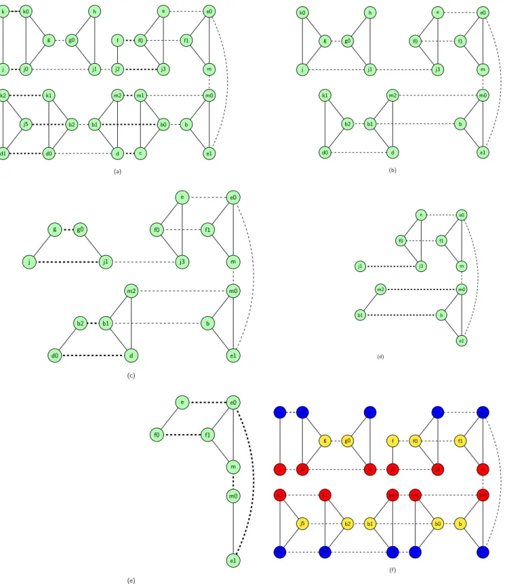
Figure 4 presents the succession of parallel cliques detected during the application of live-range unsplitting to the second graph of Figure 2, for k≥ 3. Each of the steps of Figure 4 is followed by a (traditional) phase of deletion of low-degree vertices that is not detailed in the Figure (except the first one).
At the first step four pairs parallel-cliques are detected (graph (a)), and thus coalesced. In the graph, this coalescing corresponds to the merge of four affinity edges that are in bold in graph (a): (k, k0), (j, j0), (f, f 0), (j2, j3). Graph (b) shows the graph re-sulting from this merge. In Figure 4, when two nodes are merged, the resulting node is identified by one of these two nodes (e.g. k0 in graph (b)), not to overload the graphs of Figure 4. Then, low-degree vertices (h, k0, k1) are removed, thus yielding graph (c). A new phase of parallel cliques detection is performed on graph (c),
Algorithm 2 graph reduction (G) Require: A split interference graph G Ensure: A reduced split interference graph
1: compute statement cliques
2: for allstatement clique i do
3: Ni:={statement cliques linked to i with an affinity edge}
4: end for
5: red:= 1
6: while red6= 0 do
7: red := 0
8: for allSB-clique i do
9: for all j∈ Nisuch that|i| ≥ |j| do
10: M:= dominant affinity matching(i, j)
11: if M6= N U LL then
12: merge each pair of M and compute new
weights 13: red := red+1 14: Nij:= Ni∪ Nj− {i, j} 15: for all k∈ Ni∪ Njdo 16: Nk:= Nk∪ {ij} − {i, j} 17: end for 18: end if 19: end for 20: end for
21: red := red + card({low-degree vertices})
22: remove low-degree vertices
23: end while
thus yielding the graph (d). The process is then iterated, thus yield-ing graph (e) and an empty graph.
Finally live-range unsplitting yields an empty graph, meaning that this instance can be optimally solved in polynomial time. Indeed, contrary to classical algorithms, it does not always lead to an empty graph. However, when it does, as for this example, it also ensures the optimality of the coalescing. Moreover, the solution requires only three colors while any coalescing technique applied to the the classical interference graph (first graph of Figure 2), and satisfying its two affinities, would require at least four colors. In Figure 4, thanks to live-range splitting, k and k2 are not colored with the same color, as well are j and j5.
Actually, if j and b are coalesced and if jb is the vertex obtained by coalescing j and b, then {e, f, m, jb} form a clique of four vertices. Thus these four vertices must have different colors, and four colors (at least) are needed. It shows, again, that live-range splitting can provide better solutions because variables belonging to split live-ranges may be stored in different registers.
4.
A strategy for optimal coalescing
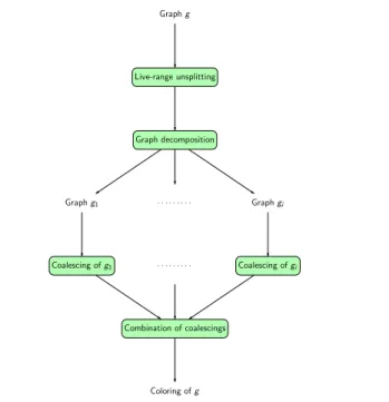
Live-range unsplitting is the first step of our strategy for optimal coalescing. This strategy consists of four steps, and it does not affect the global quality of coalescing (and preserve the optimality of coalescing). It is detailed in Figure 5.
The second step uses clique separators to decompose the graph into several smaller subgraphs. The third step consists in solving coalescing separately on each subgraph using any well-known co-alescing algorithm (i.e. a heuristic or an exact algorithm, such as an ILP). The last step is the combination of coalescings of the sub-graphs, that is the construction of the global coalescing from the coalescings of all the subgraphs.
4.1 Decomposition by clique separators
Our graph decomposition (the second step) is an enhancement of a decomposition based on clique separators that is commonly
Live-range unsplitting Graph decomposition Coalescing of g1 Coalescing of gi Combination of coalescings Graph g Graph g1 Graph gi Coloring of g . . . . . . . .
Figure 5. The whole process for coalescing.
used in operations research [22, 17]. Its main idea is to use SB-cliques, that have already been computed by the previous phase as separation sets. A separation set is a set of vertices whose removal partitions a connected component into several smaller ones. Thanks to separation cliques, coalescing needs to be solved only on each component resulting from the decomposition (and not on the whole graph), as the following property proves.
Property 1. Let s be an interference clique of g that separates g into components c1, . . . , cjand let col1, . . . , coljbe some
respec-tive colorings of c1∪s, . . . , cj∪s and colsa coloring of s. Then,Πi
is defined, for1 ≤ i ≤ j, as a permutation of {1, . . . k} such that for each vertex v of s,Πi(coli(v)) = cols(v). Such permutations
exist, since all the available colorings of a clique are permutating. The composition ofΠiand coliis thus a coloring of cisatisfying
exactly the same preferences than coli. Moreover, the coloring col
defined such that∀x ∈ ci, col(x) = Πi(coli(x)) is a coloring of g.
In other words, this property explains that it is always possi-ble to paste the colorings of subgraphs to obtain the coloring of the initial graph. A prerequisite to make the colorings of subgraphs compatible is to take care that the color of any vertex belonging to the separation clique does not change between these colorings. This constraint of compatibility can be either imposed when the co-alescing algorithm is called, by forcing the coloring of the vertices of separation cliques, or after the colorings, by permutating colors as Property 1 explains.
In split interference graphs, this decomposition can be done in linear time, rather than in quadratic time. Indeed, the hardest task is to find interference clique separators. This can easily been done in split interference graphs since all interference cliques are disjoint. Hence, to know if a SB-clique is a separator clique, we create a graph where a vertex represents a SB-clique and two vertices are adjacent if there exists an affinity edge between the two SB-cliques that these vertices represent. Then, we compute separator vertices of this graph. A separator vertex of this graph corresponds to a separator clique of the split interference graph.
Furthermore, our live-range unsplitting is based on cliques merging (see Algorithm 1) and thus makes cliques more likely
g g0 h j1 e e0 f1 m m0 b e1 k j k0 j0 k1 b2 d0 k2 j5 d1 m1 b0 c m2 b1 d (a) f j2 f0 j3 g g0 j1 j e f0 j3 e0 f1 m m0 b e1 b2 d0 m2 b1 d h k0 k1 (b) e f0 e0 f1 m m0 b e1 m2 j3 g g0 j1 j b2 d0 b1 d (c) e f0 e0 f1 m e1 j1 j3 m2 m0 b1 b (d) m e1 m0 e f0 e0 f1 (e) k k0 h e e0 e1 c d d0 d1 g g0 f f0 f1 b1 b b2 b0 j5 j1 m m0 j j0 k1 k2 m2 m1 j2 j3 (f)
(P ) 8 > > > > > > > > > > < > > > > > > > > > > : M in X (i,j)∈A wij· yij under constraints (C1) ∀i ∈ {1, . . . , n(G)}, k X c=1 xic = 1 (C2) ∀(i, j) ∈ I, ∀c ∈ {1, . . . , k}, xic+ xjc ≤ 1 (C3) ∀(i, j) ∈ A, ∀c ∈ {1, . . . , k}, xic− xjc ≤ yij (C4) ∀i ∈ {1, . . . , n(G)}, ∀c ∈ {1, . . . , k}, xic∈ {0, 1}
Figure 6. ILP formulation of Grund and Hack for coalescing. Variables are xicwhich are set to 1 iff the vertex i is of color c and yijwhich
are set to 1 iff vertices i and j have the same color. wijis the weight of the affinity edge(i, j), I is the set of interference edges, A is the set
of affinity edges and n(G) is the number of vertices of G.
to be separators. Indeed, if a union of two cliques is a separable set, then the clique obtained by merging these two cliques is a separation clique, even if the two cliques alone are not.
The strength of this decomposition is that it gets rid of solutions that are permutations of previous solutions, while reducing the size of each subproblem we need to solve. For a coloring problem, the huge number of such permutations makes this problem hard to deal with. Thus imposing a same coloring for the clique separators reduces a lot the number of solutions. Since ILP solvers are very sensitive to permutations, deleting some of them may lead to much faster optimal computations.
4.2 Impact on the cutting-plane algorithm for coalescing Even if any coalescing algorithm can be used after our strategy, this section focuses on the most efficient optimal algorithm, the cutting-plane algorithm of [16]. This algorithm consists on an ILP formu-lation of coalescing to which are added some efficient inequalities called cuts. Figure 6 recalls the formulation of [16] that we reuse.
At each iteration where a dominated parallel clique of size s is found, the size of the graph decreases of s vertices, s2interference
edges and at least s affinity edges. On the ILP formulation of [16], it involves a reduction of at least k· s + s variables (k · s for vertices and at least s for affinity edges) and at least s2+ k · s·(s−1)
2 + s
constraints (s2 for constraints C2, k· s·(s−1)2 for constraints C3
and s for constraints C1). Such a reduction is quite significant,
especially when applied many times as live-range unsplitting. Moreover, the number of cut inequalities generated for the cutting-plane algorithm and the number of variables involved in them decrease with the size of the graph. The more cut inequali-ties are generated, the more the solver takes time to find efficient ones for each iteration of the simplex algorithm (on which solvers rely). Following the same idea, the more variables are involved in a cut inequality, the more it is difficult to find values for these vari-ables. For instance, a path cut [16] is more efficient if it concerns a path of three affinity edges than if it concerns a path of ten affinity edges. For these reasons, the computation of cut inequalities and the solution are speeded up when using our strategy.
5.
Experimental results
As mentioned previously, we use the OCC as benchmark. The OCC is a set of 474 large interference graphs that result from a spilling phase. The graphs in OCC are from compiling real pro-grams in SML/NJ. The mix of easy and hard problems in OCC exactly corresponds to (inlined) functions in a set of real programs. Our strategy is applied on the OCC graphs and generates simpli-fied graphs that are given as input to the ILP formulation (and the associated cutting-plane algorithm) defined in [16]. We use the AMPL/CPLEX 9.0 solver (as in [16]) on a PENTIUM 4 2.26Ghz.
Initial nb Nb of Vertex nb Edge nb
of vertices instances ratio ratio
0-499 292 18% 33%
500-999 97 14% 27%
1000-2999 63 13% 27%
over 3000 22 13% 8%
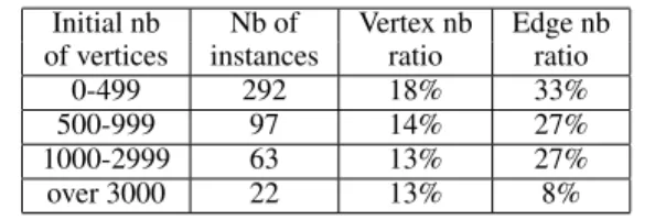
Figure 7. Size reductions for OCC graphs. The vertex (resp. edge) number ratio is the ratio between the number of vertices (resp. edges) of the largest subgraph after reduction and the one before reduction.
The first part of this section measures the efficiency of our re-duction. Then, the section details respectively optimal and near-optimal solutions.
5.1 Reduction and decomposition
The first measure is the ratio between the sizes of the OCC graph and the largest subgraph on which coalescing has to be solved (i.e. resulting from our decomposition). We focus on this subgraph because its solution requires almost the whole computation time. These results are detailed in Figure 7.
The average reduction is quite significant since the vertex (resp. edge) number is divided by 7 (resp. 4.5) when using our strategy. The reduction rates are also quite significant on the largest graphs of OCC (they are even better on the largest graphs). Let us note that the precolored vertices are always kept (because they model the calling conventions of the processor), thus involving a smaller reduction ratio for small graphs. 90% of the reduction arises from the live-range unsplitting, i.e. from the deletion of a set of splitting points. Hence, this coalescing strategy is both optimality conserva-tive and very efficient. Moreover, our algorithms run very fast since they only take 6 seconds when applied to all the instances of OCC. 5.2 Optimal solutions
We compute optimal solutions for each component of the decom-position using the cutting-plane algorithm of Grund and Hack [16]. For each interference edge, we only compute the path cut corre-sponding to the shortest path of affinity edges linking its endpoints. Figure 8 shows a fall of computation times between the solution with and without our strategy. Indeed, the cutting-plane algorithm finds only 430 optimal solutions within 5 minutes for each when ap-plied to the OCC graphs. When using our strategy combined with the cutting-plane algorithm, we find the optimal solution for 436 in-stances withing one second for each. Furthermore, only 6 inin-stances are solved in more than one minute, and only 3 of them are solved in more than 150 seconds.
0 50 100 150 200 250 300 350 400 450 500 0 20 40 60 80 100 120 140 Instances solved
Time (in seconds)
With our strategy Without
Figure 8. Number of instances of the OCC solved within a short time limit : comparison of the cutting-plane algorithm efficiency when using (or not) our strategy.
Figure 9 provides more details about computations times. It con-tains all the successive numbers of instances solved when using our strategy and their corresponding computation time. We compare these times with the ones required without our strategy to solve the same number of instances. This comparison only considers the 471 instances of the OCC both solved with and without our strategy. One could point out that the cutting-plane algorithm runs about 300 times faster when combined with our strategy.
Moreover, we are the first to solve the whole OCC instances optimally. Indeed, in [16] 3 solutions are far too slow to compute and thus their optimality was not certain. We have found a strictly better solution for one instance and proved that the two other solutions are optimal.
5.3 Near-optimal solutions
Many problems are solved within a few seconds. We adapt our approach to the other problems in order to avoid combinatorial explosion. Thus, we tune the ILP solver for the six instances that take more than one minute to be solved. Numerical results are presented Figure 10.
A first way of tuning the solver is to give it a time limit. Finding the optimal solution (or a near optimal one) often takes less than 10% of the computation time. The ILP formulation can call the solver a lot, even if the solver has a time limit. Thus, the computation can take more than the time limit. However, it never exceeds this limit too much since there is empirically only one call to the solver that reaches the time limit. In addition, this method can fail if no integer solution is found within the time limit.
A better way to tune the solver is to limit the gap between the expected solution and the optimum. Indeed, the solver can give at any time the gap between the current best solution and the best potential one using a bound of the latter. This method is the opposite of choosing a time limit: it sets the quality of the expected solution and evaluates the time spent to find it, instead of setting a time limit and evaluating the quality of the solution.
Results of Figure 10 give a flavor of the quality of coalescing on split interference graphs. The numbers of the first line are graph numbers that correspond to the six hardest graphs. First, a short time limit of 20 seconds provides solutions of good quality when it does not fail. Second, a time limit of 30 seconds leads to near-optimal coalescing. The gap between the corresponding solutions and the optimum is never greater than 20%. The failure that occurs
Nb of solved Time with Time without Time ratio
instances our strategy our strategy without/with
436 1 298 298 446 2 636 318 448 3 732 244 450 4 1198 300 451 5 1228 245 453 6 3153 525 455 7 3321 474 456 8 3574 447 458 10 4022 402 460 12 5630 469 461 15 7214 480 463 16 8709 544 464 24 10397 433 465 37 11757 317 466 40 14941 373 467 59 24916 422 468 74 25490 344 469 76 25663 337 470 133 69956 525 471 11026 71208 7
Figure 9. Time comparisons (in seconds) when using (or not) our strategy for the 471 instances of the OCC solved in both cases.
for some instances is quite prohibitive but the time limit gives a good idea of the difficulty for solving an instance.
Last, using a gap limit seems very powerful, especially when it is large enough to avoid combinatorial explosion. Here, a limit of 10% leads to solutions of very good quality (under 5% of gap with the optimum) and within a quite short time (less than two minutes). Giving a too restricted limit (such as 5% or less) leads to good solutions too but these solutions may be quite slower, as for the instance 387 that goes from 115 to 1187 seconds when the gap goes from 10% to 5%.
6.
Related work
Goodwin and Wilken were the first using ILP to solve register al-location [14, 15]. Their model solved in a single step both spilling and coalescing, but it failed to provide solutions for large programs. Furthermore, their model was quite difficult to handle since they tackled the problem with a machine level point of view. For in-stance, they did not model interference graphs. Since then, some improvements were added, in particular by Fu and Wilken [12], Ap-pel and George [3], or Grund and Hack [16]. ApAp-pel and George op-timally solved spilling by ILP and empirically showed that separat-ing spillseparat-ing and coalescseparat-ing does not significantly worsen the qual-ity of register allocation. Because their ILP formulation requires extreme live range splitting, they were not able to solve coalesc-ing optimally. More recently, Grund and Hack proposed a cuttcoalesc-ing- cutting-plane algorithm to solve coalescing and were the first to solve the OCC [16].
Our study reuses this previous work and introduces split inter-ference graphs, as well as properties of these graphs. Split interfer-ence graphs model precisely the live-ranges of variables. In particu-lar, split interference graphs are more accurate than the interference graphs obtained from programs in SSA forms (i.e. where each vari-able is defined only once) or from similar forms (e.g. SSI or SSU). Concerning coalescing, our strategy divides significantly the size of the interference graphs (by up to ten when measured on the OCC graphs), thus enabling us to find in a faster way more so-lutions that are optimal. In addition, our strategy can be combined
Instance 144 304 371 387 390 400 Optimum 129332 6109 1087 3450 339 1263 20s 129333 no no no 417 1388 30s 129333 no 1285 no 365 1263 10% gap 132040 6448 1094 3550 339 1263 5% gap 129342 6273 1094 3450 339 1263
(a) Values of solutions
Instance 144 304 371 387 390 400 Optimum 11026 1058 132 29543 102 75 20s 20 20 20 20 20 20 30s 30 30 30 30 30 30 10% gap 15 36 62 115 86 21 5% gap 17 64 62 1187 92 21 (b) Computation time
Figure 10. Comparison between different approaches for solving the hardest instances of OCC. no means that no solution is computed within the time limit. Times are in seconds.
with any coalescing algorithm. Iterated register coalescing, a com-monly used algorithm, becomes of better quality when embedded in our strategy. In our experiments, the cost of the solution was di-vided by three on average. One could expect that more recent and efficient heuristics lead to better solutions with the help of our strat-egy and we need to conduct more experiments in that direction.
7.
Conclusion
Our main motivation was to improve register coalescing using ILP techniques. Solving an ILP problem is exponential in time and thus reducing the size of the formulation can drastically speed up the solution. Rather than reasoning on the ILP model, we have studied the impact of extreme live-range splitting on register coalescing. The main drawback of extreme live-range splitting is that it yields huge interference graphs. However, no liveness information is lost when performing register allocation on these graphs. Thus, we have defined a strategy for simplifying these graphs in order to reduce significantly the size of the ILP formulation for coalescing. This strategy relies on a graph reduction and a graph decomposition, that exploit results from graph theory. Our strategy is general enough so that any coalescing algorithm can be used together with it.
As said in [16], all the optimizations must go hand in hand to achieve top performance. When our graph reduction and graph decomposition are combined with a cutting-plane algorithm, we solve the whole optimal coalescing challenge optimally and more efficiently than previously.
Moreover, this work on extreme live-range splitting raises many questions. Indeed, it can be interesting to relax some constraints on split-blocks merging in order to design new heuristics, or to wonder if unsplitting could be done before spilling. Finally, since finding optimal solutions for spilling and coalescing separately is not elusive anymore, one could expect to solve both simultaneously and to evaluate the real gap arising from the separation.
This work is part of an on-going project that investigates the formal verification of a realistic C compiler usable for critical embedded software. Future work concern the formal verification of the optimizations described in this paper.
Acknowledgments
We would like to thank Andrew Appel for fruitful discussions about this work.
This work was supported by Agence Nationale de la Recherche, grant number ANR-05-SSIA-0019.
References
[1] Andrew W. Appel. Modern Compiler Implementation in ML. Cambridge University Press, 1998.
[2] Andrew W. Appel and Lal George. Optimal coalescing challenge, 2000. http://www.cs.princeton.edu/~appel/coalesce. [3] Andrew W. Appel and Lal George. Optimal spilling for CISC
machines with few registers. In PLDI’01, pages 243–253, 2001.
[4] Peter Bergner, Peter Dahl, David Engebretsen, et al. Spill code minimization via interference region spilling. In PLDI ’97, pages 287–295, 1997.
[5] Florent Bouchez. A Study of Spilling and Coalescing in Register Allocation as Two Separate Phases. PhD thesis, ENS Lyon, France, dec 2008.
[6] Florent Bouchez, Alain Darte, and Fabrice Rastello. On the complexity of register coalescing. In CGO’07, mar 2007.
[7] Preston Briggs. Register Allocation via Graph Coloring. PhD thesis, Rice University, april 1992.
[8] Philip Brisk, F.Dabiri, J.Macbeth, et al. Polynomial time graph coloring register allocation. In Workshop on Logic and Synthesis, 2005.
[9] G J Chaitin. Register allocation and spilling via graph coloring. Symposium on Compiler Construction, 17(6):98 – 105, 1982. [10] Fred C. Chow and John L. Hennessy. The priority-based coloring
approach to register allocation. ACM TOPLAS, 12(4):501–536, 1990. [11] Keith D. Cooper and L. Taylor Simpson. Live range splitting in a
graph coloring register allocator. In CC ’98, pages 174–187, 1998. [12] Changqing Fu and Kent Wilken. A faster optimal register allocator.
In MICRO 35, pages 245–256, 2002.
[13] Lal George and Andrew W. Appel. Iterated register coalescing. ACM TOPLAS, 18(3):300–324, 1996.
[14] David Goodwin and Kent Wilken. Optimal and near-optimal global register allocations using 0-1 integer programming. Softw. Pract. Exper., 26(8):929–965, 1996.
[15] David W. Goodwin. Optimal and near-optimal global register allocation. PhD thesis, University of California, 1996.
[16] Daniel Grund and Sebastian Hack. A fast cutting-plane algorithm for optimal coalescing. In CC’07, LNCS, pages 111–125, 2007. [17] Rajiv Gupta, Mary Lou Soffa, and Denise Ombres. Efficient register
allocation via coloring using clique separators. ACM TOPLAS., 16(3):370–386, 1994.
[18] Priyadarshan Kolte and Mary Jean Harrold. Load/store range analysis for global register allocation. In PLDI’93, pages 268–277, 1993. [19] Guei-Yuan Lueh and Thomas Gross. Fusion-based register allocation.
ACM TOPLAS, 22:2000, 1997.
[20] Jinpyo Park and Soo-Mook Moon. Optimistic register coalescing. In PACT ’98, page 196, 1998.
[21] Vivek Sarkar and Rajkishore Barik. Extended linear scan: An alternate foundation for global register allocation. In CC’07, LNCS, pages 141–155, 2007.
[22] Robert Endre Tarjan. Decomposition by clique separators. Discrete Mathematics, 55(2):221–232, 1985.
[23] Douglas B. West. Introduction to Graph Theory (2nd Edition). Prentice Hall, August 2000.
[24] Mihalis Yannakakis and Fanica Gavril. The maximum k-colorable subgraph problem for chordal graphs. Inf. Process. Lett., 24(2):133– 137, 1987.