Application of chemical mass balance modeling to indoor VOCs

(1)

READ THESE TERMS AND CONDITIONS CAREFULLY BEFORE USING THIS WEBSITE.

https://nrc-publications.canada.ca/eng/copyright

Vous avez des questions? Nous pouvons vous aider. Pour communiquer directement avec un auteur, consultez la

première page de la revue dans laquelle son article a été publié afin de trouver ses coordonnées. Si vous n’arrivez pas à les repérer, communiquez avec nous à PublicationsArchive-ArchivesPublications@nrc-cnrc.gc.ca.

Questions? Contact the NRC Publications Archive team at

PublicationsArchive-ArchivesPublications@nrc-cnrc.gc.ca. If you wish to email the authors directly, please see the first page of the publication for their contact information.

NRC Publications Archive

Archives des publications du CNRC

This publication could be one of several versions: author’s original, accepted manuscript or the publisher’s version. / La version de cette publication peut être l’une des suivantes : la version prépublication de l’auteur, la version acceptée du manuscrit ou la version de l’éditeur.

Access and use of this website and the material on it are subject to the Terms and Conditions set forth at

Application of chemical mass balance modeling to indoor VOCs

Won, D. Y.; Shaw, C. Y.; Biesenthal, T. A.; Lusztyk, E.; Magee, R. J.

https://publications-cnrc.canada.ca/fra/droits

L’accès à ce site Web et l’utilisation de son contenu sont assujettis aux conditions présentées dans le site LISEZ CES CONDITIONS ATTENTIVEMENT AVANT D’UTILISER CE SITE WEB.

NRC Publications Record / Notice d'Archives des publications de CNRC:

https://nrc-publications.canada.ca/eng/view/object/?id=5196dc96-c13c-4c71-86fe-06e759c6640f https://publications-cnrc.canada.ca/fra/voir/objet/?id=5196dc96-c13c-4c71-86fe-06e759c6640f

(2)

indoor VOCs

Won, D.; Shaw, C.Y.; Biesenthal, T.A.; Lusztyk, E.; Magee, R.J.

A version of this document is published in / Une version de ce document se trouve dans : Proceedings: Indoor Air 2002, Monterey, CA., U.S.A., June 30-July 5, 2002, pp. 268-273

www.nrc.ca/irc/ircpubs

(3)

APPLICATION OF CHEMICAL MASS BALANCE MODELING TO

INDOOR VOCS

D Won*, CY Shaw, TA Biesenthal, , E Lusztyk, and RJ Magee

Institute for Research in Construction, National Research Council, Ottawa, Ontario, Canada

ABSTRACT

There have been several studies to measure the concentrations of volatile organic compounds (VOCs) indoors and to characterize their sources. However, the two tasks have often been done separately, and few attempts have been made to provide a direct link between the

sources and the measured VOCs. Chemical mass balance (CMB) modeling was applied to the measurements of 24 VOCs in a newly constructed house. The results of CMB modeling show that wall adhesive, caulking, I-beam joist, and particleboard are the dominant sources. An attempt was also made to estimate the source contributions using mathematical transport modeling. Good agreement was obtained between the two results. The CMB model is shown to have good potential for identifying the dominant sources and helping develop control strategies for indoor VOCs. However, more research is needed for the collinearity problem associated with source signatures.

INDEX TERMS

Source apportionment, Chemical mass balance, VOCs, Indoor air, Building materials INTRODUCTION

The chemical mass balance (CMB) model, a source apportionment technique, has been widely used in outdoor air pollution studies to identify emission sources responsible for the measured concentrations of particulates and VOCs (Henry et al., 1984; Waston, Chow, and Fujita, 2001). This information has been found to be useful in developing pollution control strategies. However, there have been few attempts to apply the CMB model to indoor air quality studies to link emission sources with measured VOCs in the air.

Source apportionment techniques attempt to identify the contributions of sources responsible for the chemical compounds identified at a sampling site based on the measured

concentrations. These techniques are also referred to as receptor modeling. On the other hand, mathematical transport modeling, which has been frequently used in indoor air quality studies, estimates the contributions of emission sources to the chemical concentrations in the air based on fundamentals of chemistry and physics (Seinfeld and Pandis, 1997). Since receptor modeling considers the transport mechanism between sources and receptors as a black box, it needs little or no prior information on sources and transport processes. The objective of this study is to show the applicability of CMB modeling to indoor air quality studies by identifying dominant indoor sources based on the measured VOC concentrations in the air.

*

Contact author email: doyun.won@nrc.ca

Proceedings: Indoor Air 2002

(4)

METHODS

Chemical mass balance model

The concentration of a pollutant at a sampling location can be considered as the summation of the contributions from various sources:

m i s a x _j p j ij i =

∑

=1,..., (1)

where xi is the predicted concentration of pollutant i at a sampling location,

aij is the source signature for pollutant i from source j, which will be obtained from

a material emissions database developed by Institute for Research in Construction,

sj is the contribution of source j, which is the unknown and to be solved,

m is the number of pollutants, and p is the number of sources.

The value of sj can be found by minimising the difference between the measured (Ci) and the

predicted (xi) concentrations:

∑

      − = m i j p j ij i i s a C 2 2 2 1 ₍ ₎ σ ξ (2)

This is the common multiple regression analysis problem (Seinfeld and Pandis, 1997). When the uncertainties (σi) in the measurements are assumed to be constant among pollutants, the solution method is referred to as least squares. The least squares solution of Eq. 2 is the vector s of source contributions given by Eq. 3.

[ ]

A A A c

s= T −1 T (3)

where A is the m × p source signature matrix with the source composition aij, AT is the transpose matrix of A,

c is the vector with the concentration measurements.

The solution vector s was obtained for 20 sets of VOC measurements and was averaged later. Application to VOC field measurements

VOC concentration measurements were obtained during and after the construction of the "Reference" house, which is one of two research houses under the project of the Canadian Center for Housing Technology (CCHT). Air samples in the house were collected on Carbotrap 300 sorbent tubes followed by thermal desorption and GC/MS analysis. The quantification for each VOC was based on the response curve of toluene. A total of twenty samples were collected between 127 and 311 days after the foundation of the house was poured.

Since the house was newly constructed and unoccupied, only building materials were

considered as sources. The average source signatures were obtained for materials in the same category from the material emissions database developed by Institute for Research in

Construction. This type of general source signatures is useful, considering that source signatures for specific materials of interest in most test houses are unlikely to be readily available.

(5)

Table 1. Source signature (aij) for 24 VOCs from 10 building materials

Concentration/Sum of concentrations of 24 VOCs

VOCs _WSa

GB a OSB a CRP a WV a IBJ a CK a PLY a PB a AD a

Benzene, 1-ethyl-3-methyl- - 0.007 - - - - 0.034 - - 0.023 Benzene, 1,2,3-trimethyl- - 0.009 - - - - 0.037 - - 0.041 Benzene, 1,2,4-trimethyl- - 0.021 - - - - 0.049 - - 0.045 Camphene - 0.002 - - - 0.075 - 0.048 0.172 - 3-Carene - - - - - 0.141 0.064 - Cyclohexane, butyl- 0.069 - - - 0.026 - 0.037 - - 0.036 Cyclohexane, 1,1,2,3-tetramethyl 0.058 - - - - - 0.043 - - 0.011 Cyclohexane, prophyl- 0.058 - - - - - 0.040 - - 0.017 Decane 0.203 0.069 - 0.065 0.288 - 0.265 0.052 - 0.265 Decane, 3-methyl 0.048 0.010 - - 0.061 - 0.033 - - 0.027 Decane, 4-methyl 0.039 0.012 - - - - 0.023 - - 0.035 Dodecane 0.065 0.017 - 0.103 0.022 - 0.027 - - 0.041 Hexanal - 0.009 0.918 - - 0.004 - 0.084 0.054 - Limonene - 0.003 - 0.041 - 0.064 0.006 0.263 0.145 - Nonane 0.136 0.010 - - 0.154 - 0.104 0.031 - 0.082 Nonane, 2-methyl- 0.060 0.005 - - 0.034 - 0.046 - - 0.025 Nonane, 3-methyl- 0.093 0.005 - - 0.040 - 0.054 - - 0.029 Nonane, 4-methyl- 0.060 0.007 - - 0.030 - 0.055 - - 0.030 α-Pinene - 0.011 0.041 - - 0.713 - 0.251 0.500 - β-Pinene - 0.727 - - - 0.144 - 0.112 0.065 - Toluene - - 0.010 0.033 - - 0.010 0.007 - - Undecane 0.109 0.074 0.031 0.108 0.346 - 0.127 0.010 - 0.278 Undecane, 2-methyl- - - - - 0.010 - - - p-Xylene - - - 0.650 - - - - - 0.013 Sum 1.000 1.000 1.000 1.000 1.000 1.000 1.000 1.000 1.000 1.000

a_{WS: wood stain (2), GB: gypsum board (3), OSB: oriented strand board (4), CRP: carpet (6), WV:}

wood varnish (1), IBJ: I-beam (1), CK: caulking (2), PLY: plywood (4), PB: particleboard (3), AD: wall adhesive (1). The value in parenthesis is the number of materials used for averaging.

RESULTS

Source contributions by CMB modeling

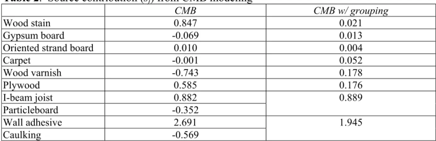
The results of CMB modeling are listed in Table 2. The negative values of source

contributions in the second column are most likely due to the similarities in source signatures. The collinearity problem is not uncommon in CMB and can result in large uncertainties as well as negative values for estimated source contributions (Henry et al., 1984).

Table 2. Source contribution (sj) from CMB modeling

CMB CMB w/ grouping

Wood stain 0.847 0.021 Gypsum board -0.069 0.013 Oriented strand board 0.010 0.004

Carpet -0.001 0.052 Wood varnish -0.743 0.178 Plywood 0.585 0.176 I-beam joist 0.882 Particleboard -0.352 0.889 Wall adhesive 2.691 Caulking -0.569 1.945

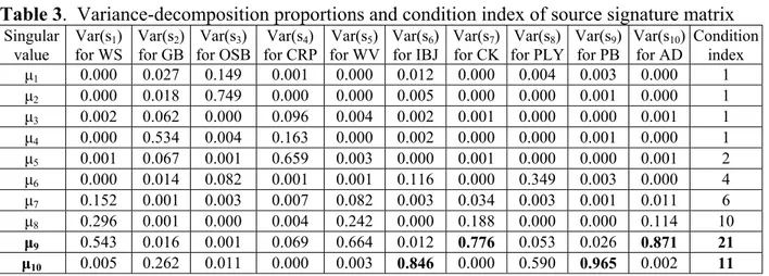
It is suggested that each near linear dependence among the vectors of the source signature matrix A will manifest itself in a small singular value, which is the square root of eigenvalue of ATA (Belsely et al., 1980). Therefore, condition number (µ), i.e., the ratio of the maximum

(6)

singular value to a singular value of A, can be adopted as a measure of collinearity. Belsely

et al. (1980) employed the condition index threshold of 10 for weak dependencies. The

analysis for variance-decomposition proportions can be another measure of collinearity. The estimated variance of each regression coefficient may be decomposed into a sum of terms each of which is associated with a singular value, thereby providing means for determining the extent to which near dependencies degrade each variance. Consequently, the dependent source signatures can be identified by the joint occurrence of high variance-decomposition proportions for two or more coefficients associated with a single singular value having a "high" condition index (Belsley et al., 1980).

Systat 10 was used to calculate variance-decomposition proportions and condition indexes for the source signature matrix A (Table 3). The condition index of 21 suggests that there are weak or moderate dependencies among some source signatures. The value of 0.7 was employed as the cut-off for the high value of variance-decomposition proportions to identify sources of collinearity. The 9th singular value accounts for 70% or more of Var(s7) and Var(s10), which indicates that source signatures of caulking and wall adhesive are similar enough to cause collinearity. Additionally, the 10th singular value accounts for 80% or more of Var(s6) and Var(s9), which also suggests that I-beam joist and particleboard have similar source signatures.

Table 3. Variance-decomposition proportions and condition index of source signature matrix

Singular value Var(s1) for WS Var(s2) for GB Var(s3) for OSB Var(s4) for CRP Var(s5) for WV Var(s6) for IBJ Var(s7) for CK Var(s8) for PLY Var(s9) for PB Var(s10) for AD Condition index µ1 0.000 0.027 0.149 0.001 0.000 0.012 0.000 0.004 0.003 0.000 1 µ2 0.000 0.018 0.749 0.000 0.000 0.005 0.000 0.000 0.001 0.000 1 µ3 0.002 0.062 0.000 0.096 0.004 0.002 0.001 0.000 0.000 0.001 1 µ4 0.000 0.534 0.004 0.163 0.000 0.002 0.000 0.000 0.001 0.000 1 µ5 0.001 0.067 0.001 0.659 0.003 0.000 0.001 0.000 0.000 0.001 2 µ6 0.000 0.014 0.082 0.001 0.001 0.116 0.000 0.349 0.003 0.000 4 µ7 0.152 0.001 0.003 0.007 0.082 0.003 0.034 0.003 0.001 0.011 6 µ8 0.296 0.001 0.000 0.004 0.242 0.000 0.188 0.000 0.000 0.114 10 µ9 0.543 0.016 0.001 0.069 0.664 0.012 0.776 0.053 0.026 0.871 21 µ10 0.005 0.262 0.011 0.000 0.003 0.846 0.000 0.590 0.965 0.002 11

Hopke et al. (1984) suggests that grouping similar sources may provide a solution, although the resolution of the source apportionment is compromised. Based on the results of Table 3, caulking and wall adhesive were grouped into one source with the averaged source signature. The maximum value of condition index was lowered to 13, but some of source contributions remained negative. Additional grouping for I-beam joist and particleboard lowered the maximum value of condition index to 12 and provided non-negative source contributions (Table 2). The R2 value for CMB modeling with 8 sources was 0.82, which is greater than the threshold of 0.8 suggested in Waston, Chow, and Pace (1991).

Comparison to source contributions by mathematical simulation modeling

The source contributions obtained from CMB modelling were compared to those estimated from a single zone mathematical simulation (SMS) model. Simulation was conducted for each of the 10 sources (materials) individually. The source contributions by the SMS model were determined on the percentage basis by normalizing the concentration from each source by the total concentrations from all sources. Table 4 provides input data for the SMS model, including emission models for total VOC, area of sources, and input time of each source into

(7)

the house. For dry materials, the power law decay model was used (Eq. 4). Three different models used for wet materials: the evaporation controlled model (Eq. 5) for 0<t<t1, the exponential decay model (Eq. 6) for t1<t<t2, and the power law decay model (Eq. 4) for t>t2.

b t a E= − (4) ) 0 ( ) ( ) ( 1 01 t t t C M t M C K E _m _v _ < <            − = (5) ) ( ) (_t₁ _e ( 1) _t₁ _t _t₂ E E= −kt−t < < (6)

where a and b are empirical constants, t is the elapsed time (h),

Km is the convective mass transfer coefficient (m2 h-1),

Cv is the initial surface concentration (mg m-3),

M01 is the initial mass available for evaporation (mg m-3),

E(t1) is the emission factor at t = t1,

k is the emission decay constant,

t1 is the time at which the transition period began (h),

t2 is the time at which the diffusion controlled period began (h).

The volume of the house is 794.3 m3 and the air change rate is 50 h-1 (0 - 106 days), 0.25 h-1 (107 - 155 days), and 0.23 h-1 (156 - 311 days).

Table 4. Input data for the single-zone mathematical model Area (m2) In Time (d) t1 (h) Mo1 (mg m-2) Km (m h-1) Cv (mg m-3) t2 (h) E(t1) (mg m-2 h-1) k (h-1) a b WS a 5 102 7 40237.42 1.13 39111 24 294.72 0.11811 16024 1.8891 283.2 101 - - - - - - - 31.979 1.063 GB 283.2 102 - - - - - - - 31.979 1.063 34.8 9 - - - - - - - 1.509 0.3201 34.8 10 - - - - - - - 1.509 0.3201 OSB 5.56 168 - - - - - - - 1.509 0.3201 63.5 116 - - - - - - - 7.414 0.8421 CRP 63.5 119 - - - - - - - 7.414 0.8421 WV 5 123 7 78676.46 1.13 62556 24 915.17 0.1618 2875.5 1.2261 28.7 9 - - - - - - - 64.818 0.6264 IBJ 28.7 10 - - - - - - - 64.818 0.6264 CK 0.1 76 4 199366 1.13 78055 24 15078 0.022997 59810 0.5783 PLY 5.56 105 - - - - - - - 57.39 1.4222 PB 1.5 30 - - - - - - - 25.108 0.395 AD 0.1 105 2 13229.94 1.13 2056.4 24 1615 0.00368 31512 0.9602

a_{WS: wood stain, GB: gypsum board, OSB: oriented strand board, CRP: carpet, WV: wood varnish,}

IBJ: I-beam joist, CK: caulking, PLY: plywood, PB: particleboard, AD: wall adhesive.

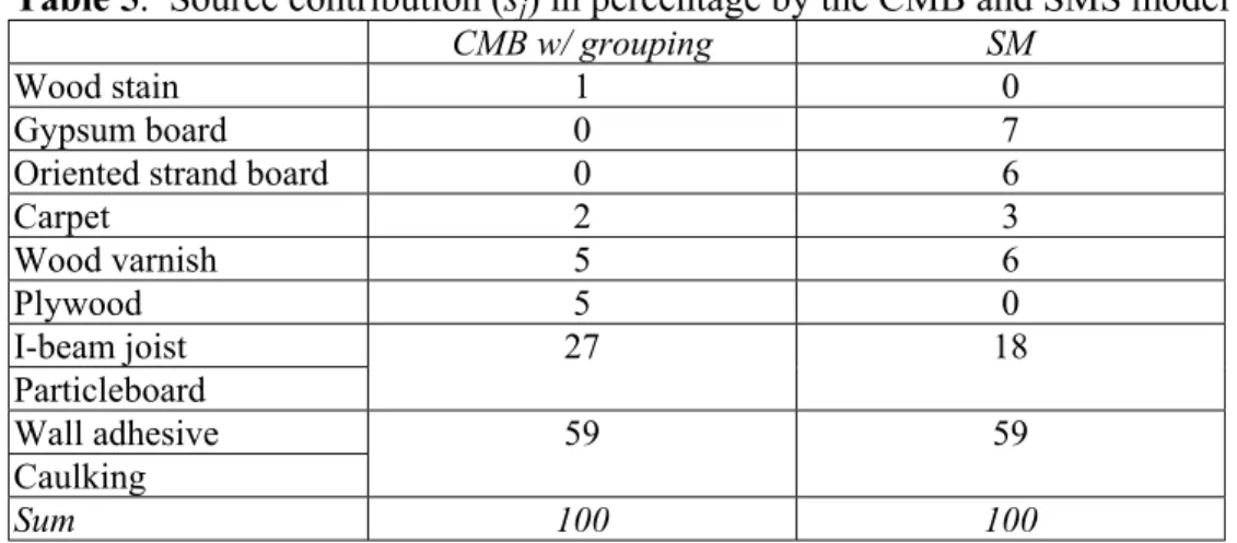
The relative source contributions (%) by the CMB model with grouping and the SMS model are compared in Table 5. The group of caulking and wall adhesive is shown to be the most dominant source with 59% contribution by both models. The second dominant source group is predicted to be I-beam joist and particleboard by two models, although the magnitude of the contribution is different each other. The four sources, i.e., caulking, wall adhesive, I-beam joist, and particleboard, appear to account for 86% (CMB) and 77% (SMS) of VOCs in the house. The next dominant sources are identified to be wood varnish and plywood by the CMB model, while they are gypsum board, wood varnish, and oriented strand board by the SM model. Wood stain and carpet are predicted to be insignificant sources by both models. The agreement in source contributions between the CMB and SMS model is concluded to be

(8)

very good, considering the fact that source signatures for the CMB model are the averages of several materials in the same category and the source model for the SM model is based on one material.

Table 5. Source contribution (sj) in percentage by the CMB and SMS model

CMB w/ grouping SM

Wood stain 1 0 Gypsum board 0 7 Oriented strand board 0 6

Carpet 2 3 Wood varnish 5 6 Plywood 5 0 I-beam joist Particleboard 27 18 Wall adhesive Caulking 59 59 Sum 100 100

CONCLUSION AND IMPLICATIONS

Chemical mass balance modelling was applied to identify the dominant sources of VOCs in indoor air in a newly constructed house. Chemical mass balance modeling identified four dominant sources including caulking, wall adhesive, I-beam joist, and particleboard. The results agree well with those by single zone mathematical simulation modeling. This shows that chemical mass balance modeling has a potential in identifying the most influential sources of VOCs in indoor air based on the VOC measurements and published dynamic emission test results on individual materials. However, it was shown that similar source signatures could cause collinearity, which can result in unrealistic source contributions. Therefore, more research on handling the collinear problem is needed for more general application of chemical mass balance modeling to VOCs indoors.

REFERENCES

Belsley DA, Kuh E, Welsch RE. 1980. Regression diagnostics: Identifying influential data

and sources of collinearity. New York: John Wiley & Sons.

Henry RC, Lewis CW, Hopke PK, and Williamson HJ. 1984. Review of receptor model fundamentals. Atmospheric Environment, Vol. 18(8), pp 1507-1515.

Seinfeld JH, and Pandis SN. 1997. Atmospheric Chemistry and Physics. John Wiley and Sons. Watson JG, Chow JC, and Fujita EM. 2001. Review of volatile organic compound source

apportionment by chemical mass balance. Atmospheric Environment, Vol. 35, pp 1567-1584.

Watson JG, Chow JC, and Pace TG. 1991, Chemical mass balance. In Receptor Modeling for