Masking speech in open-plan offices with simulation ventilation noise: noise-level and spectral composition effects on acoustic satisfaction

(1)

Publisher’s version / Version de l'éditeur:

Vous avez des questions? Nous pouvons vous aider. Pour communiquer directement avec un auteur, consultez la première page de la revue dans laquelle son article a été publié afin de trouver ses coordonnées. Si vous n’arrivez pas à les repérer, communiquez avec nous à PublicationsArchive-ArchivesPublications@nrc-cnrc.gc.ca.

Questions? Contact the NRC Publications Archive team at

PublicationsArchive-ArchivesPublications@nrc-cnrc.gc.ca. If you wish to email the authors directly, please see the first page of the publication for their contact information.

https://publications-cnrc.canada.ca/fra/droits

L’accès à ce site Web et l’utilisation de son contenu sont assujettis aux conditions présentées dans le site LISEZ CES CONDITIONS ATTENTIVEMENT AVANT D’UTILISER CE SITE WEB.

Internal Report (National Research Council of Canada. Institute for Research in

Construction), 2002-04-01

READ THESE TERMS AND CONDITIONS CAREFULLY BEFORE USING THIS WEBSITE. https://nrc-publications.canada.ca/eng/copyright

NRC Publications Archive Record / Notice des Archives des publications du CNRC : https://nrc-publications.canada.ca/eng/view/object/?id=7b46ed82-9360-424c-92f1-47cde0e2620b https://publications-cnrc.canada.ca/fra/voir/objet/?id=7b46ed82-9360-424c-92f1-47cde0e2620b

Archives des publications du CNRC

For the publisher’s version, please access the DOI link below./ Pour consulter la version de l’éditeur, utilisez le lien DOI ci-dessous.

https://doi.org/10.4224/20386334

Access and use of this website and the material on it are subject to the Terms and Conditions set forth at

Masking speech in open-plan offices with simulation ventilation noise:

noise-level and spectral composition effects on acoustic satisfaction

Veitch, J. A.; Bradley, J. S.; Legault, L. M.; Norcross, S. G.; Svec, J. M.

(2)

Composition Effects on Acoustic Satisfaction

Veitch, J.A.; Bradley, J.S.; Legault, L.M.;

Norcross, S.; Svec, J.M.

www.nrc.ca/irc/ircpubs

IRC-IR-846

(3)

Noise: Noise Level and Spectral Composition Effects on Acoustic

Satisfaction

by Jennifer A. Veitch, John S. Bradley, Louise M. Legault, Scott Norcross,

& Jana M. Svec

Internal Report No. IRC-IR-846

Date of issue: April 2002

This internal report, while not intended for general distribution, may be cited or referenced in other publications.

(4)

Masking Speech in Open-Plan Offices with Simulated Ventilation Noise:

Noise Level and Spectral Composition Effects on Acoustic Satisfaction

Jennifer A. Veitch

John S. Bradley

Louise M. Legault

Scott Norcross

Jana M. Svec

Institute for Research in Construction

National Research Council Canada

Montreal Road, Ottawa, Ontario

CANADA, K1A 0R6

Internal Report No. IRC-IR-846

April 2002

(5)

Acknowledgements

These experiments form part of the Acoustics sub-task for the NRC/IRC project Cost-effective Open-Plan Environments (COPE) (NRCC Project # B3205), supported by Public Works and Government Services Canada, Natural Resources Canada, the Building Technology Transfer Forum, Ontario Realty Corp, British Columbia Buildings Corp, USG Corp, and Steelcase, Inc. COPE is a multi-disciplinary project directed towards the development of a decision tool for the design, furnishing, and operation of open-plan offices that are satisfactory to occupants, energy-efficient, and cost-effective. Information

about COPE is available at http://www.nrc.ca/irc/ie/cope.html.

The authors are grateful to the following individuals for contributions to these experiments: Guy Newsham, Alf Warnock, David Quirt, and Wing Chu for advice in creating the acoustical conditions; Gordon Bazana for data management; Staffan Hygge (University of Gävle, Sweden, Dept. of Built Environment), for advice on tasks and dependent measures; and, Michael Hunter (University of Victoria, Dept. of Psychology), for advice concerning statistical analyses.

(6)

Masking Speech in Open-Plan Offices with Simulated Ventilation Noise:

Noise Level and Spectral Composition Effects on Acoustic Satisfaction

Executive Summary

The Cost-Effective Open-Plan Environments (COPE) project plan identified a need to develop relationships between acoustic conditions in open-plan offices and occupant satisfaction with those conditions. Two experiments were designed to meet this need. In each experiment, participants hired from a staffing agency for one day experienced 15 different simulated ventilation noises in combination with simulated telephone conversations, and provided ratings of their satisfaction with each noise condition. Each exposure consisted of a 15-minute period of work on memory and clerical tasks, followed by 2-3 minutes to complete a questionnaire concerning satisfaction, speech intelligibility, and the characteristics of the noise. This report concerns only the questionnaire data. Memory and clerical task performance in relation to the noise conditions will be reported separately.

• Experiment 1: Noise spectrum effects on satisfaction. In this experiment subjects experienced 15

different simulated noise spectra in combination with the speech from simulated telephone conversations.

• Experiment 2: Noise spectrum and noise level effects on satisfaction. This experiment used three

noise spectra at each of five A-weighted noise levels, for a total of 15 different noise conditions in combination with the speech from simulated telephone conversations.

The results of the two experiments provided guidance for identifying acoustical conditions likely to prove satisfactory to occupants:

• Acoustic satisfaction increases as subjectively rated speech intelligibility decreases. This is

consistent with our prediction, that speech privacy is what people want.

• The difference between low- and high-frequency A-weighted levels is a good predictor of the

effects of masking sound spectrum shape on acoustic satisfaction.

• Acoustic satisfaction decreases as hissiness increases. Thus, sound masking systems must balance

the need for frequency sound to mask speech, and the need to avoid excessive levels of high-frequency sound.

• Noise spectra that follow the speech spectrum are effective speech maskers.

• Louder masking noise is more effective at making speech less intelligible.

• Louder masking noise does not improve speech masking as much if the spectrum is a poor masker.

Simply making the masking noise louder is not a guarantee of improved speech privacy.

• Noise levels much greater than 45 dB(A) are judged to be too loud, even though they are more

effective at speech masking.

• Over the range of acoustic conditions in open-plan offices, Speech Intelligibility Index (SII) is a good

predictor of acoustic satisfaction and rated speech intelligibility. The findings are consistent with the rule-of-thumb that SII values greater than 0.20 are unacceptable.

(7)

1.0 Introduction

Occupants of open-plan offices frequently complain about the acoustical environment as a

significant problem involving both attention and privacy (Sundstrom, 1987; Sundstrom, Town, Rice, Osborn, & Brill, 1994). Unwanted sound from other people and from equipment is a distraction and can be a source of annoyance. The fact that office workers can hear the conversations of others or that others can hear one's own conversations is an absence of privacy. Despite the frequent reports of dissatisfaction, there is little specific information about the characteristics of the noise that people find most annoying; or, conversely, about the conditions that they find to be most satisfactory. Without this information, it is impossible to design open-plan offices to optimise satisfaction and speech privacy. This is particularly important because open offices are already the norm and there are new trends that could decrease privacy and satisfaction, such as smaller and more open work stations.

Open office acoustical problems can be broken up into two types: annoyance to various noises and a lack of speech privacy. Too much of almost any type of noise can be a source of annoyance in at least some situations. In general the level, spectrum, and variation with time of the noise will influence how disturbing it is found to be. Noise from people talking, telephones ringing, and other intermittent sounds can be more disruptive than more continuous sounds (Sundstrom et al., 1994). The more audible speech sounds from adjacent workstations are, then the less speech privacy there will be. This may be experienced as audible speech from an adjacent workstation or the perception that others can listen to ones own conversations. Generally, the quieter the intruding speech sounds and the louder various ambient noises are, then the greater the speech privacy.

Increasing ambient noise by adding a constant, information-free noise source (called masking noise) can improve the conditions within a workstation by masking speech sounds propagating from adjacent spaces. Masking noise is usually a noise of neutral quality similar to ventilation noise. Masking noise can decrease disturbance (Loewen & Suedfeld, 1992), despite the fact that the overall sound level is increased. There is obviously a limit to how loud the masking noise can be and still be judged a neutral masking sound. Increased noise levels will at some point lead to increased annoyance as well as to increased speech levels, which would further exacerbate the situation.

Unfortunately, these effects are not precisely quantified and most of our knowledge is anecdotal in character (Warnock, 1972; Warnock, Henning, & Northwood, 1972). The fundamentals of how one sound can mask another are well understood (Zwicker & Fastl, 1990) and the Speech Intelligibility Index measure (Acoustical Society of America Standards Secretariat (ASA), 1997) that is used as an indicator of speech privacy is based on our current understanding of the masking of speech sounds by other sounds. There are commercially-available masking noise systems in use in many workplaces. However, there appears to have been no systematic research published on which to base the choice of noise

characteristics, either in terms of frequency content or sound level, for open office situations (there might exist proprietary research on this topic, but by definition these are not available publicly).

This report describes a pair of experiments designed to determine the relationship of satisfaction with a range of combinations of speech and noise in an open office work situation. The research was divided into two experiments to more completely consider the many possible variations of noise spectrum and level representative of typical ventilation noises in offices. In the first experiment subjects experienced only different noise spectra at constant noise level, but in the second experiment they experienced a combination of noise spectrum and noise level.

(9)

2.0 Experiment 1: Effects of Masking Noise Spectrum on Satisfaction

2.1 Method

Because of the many possible combinations of noise spectrum shape and noise level, the first experiment was intended to first develop an understanding of the importance of noise spectrum on satisfaction ratings. In this experiment subjects experienced 15 different simulated noise spectra in combination with the speech from simulated telephone conversations.

Participants were recruited from an office temporary services supplier and paid at the standard rate for a day’s clerical work. They were tested by the supplier to ensure a minimum level of English fluency and were experienced in the use of

Windows-based word processing and spreadsheet software. The participants knew that the day's work was in support of a research project concerning the effects of the physical environment on office workers. They received advance information from the supplier (Appendix A), and completed an informed consent procedure at the start of the day at NRC (Appendix B).

Complete data were obtained from 35 participants (17 women and 18 men), ranging in age from 18 - 65 years (M=32. 9, SD=12.8). Other self-rated characteristics are reported in Table 1. Two additional participants did not complete the full day, and their data were excluded from analysis.

Table 1. Characteristics of Experiment 1 Participants. Hearing Impairment 1 = yes

34 = no Hearing Aid 1 = yes 34 = no Visual Aids 18 = none

11 = distance glasses 2 = bifocals

3 = contact lenses 1 = no response Education 21 = High school

5 = community college / CEGEP 7 = undergraduate degree 2 = graduate degree Years in work force Range 1 year - 40 years

M = 12.4 years SD = 10.3 years

Participants completed a Hughson Westlake threshold of audibility hearing test at the start of the test day. Their hearing levels relative to threshold values at 500, 1000, 2000, 3000, 4000, and 6000 Hz were summed and subjects with values greater than 20 were classified as having some hearing

impairment. The data for Experiment 1 participants, however, was uninterpretable because of an operator error during testing. One participant reported wearing a hearing aid; this person's data were retained for analysis on the basis of the self-reported correction.

The experiment took place in the Indoor Environment Research Facility (IERF) in Building M-24 on the Montreal Road Campus in Ottawa, Ontario. The IERF is a mocked-up 12.2 x 7.3 m (40 x 24 ft) office designed for acoustics, lighting, ventilation, and indoor air quality research. Interior designers at Public Works and Government Services Canada were hired to lay out the space as a typical mid-level clerical or administrative office similar to those currently being installed in Canadian government buildings (Figure 1). The result is a design having six open-plan workstations of

2.1.1 Objective.

2.1.2 Participants.

(10)

approximately 6 m2 (65 ft2) with space for shared file cabinets and printers at the end of the room. The workstations are standard modular systems furniture with computers, storage space, keyboard shelf, and adjustable-height chair. For this experiment, the room was windowless. Temperature, lighting, and ventilation remained unchanged over all experimental sessions and were within normal guidelines for office environments.

Figure 1. View of NRC's Indoor Environment Research Facility.

Up to five participants attended on one day; the sixth workstation (workstation 2, in the centre of the back row of workstations) was reserved for the simulated occupant whose speech was masked by the simulated ventilation noise that was the focus of the experiment. The experimental sessions began in the reception/lounge room outside the experimental facility (IERF). This room is equipped with comfortable chairs, a coffee area, and coatroom. The initial instructions, including the signing of the consent form, and all coffee and lunch breaks all occurred in this space. The participants then proceeded to their assigned workstations in the IERF, where the day’s work was presented on the computer. The experimenter monitored the participants during the day from the control room using the security monitoring system (video only) in the IERF. The participants were aware that the security cameras were in use and that no permanent record was kept. (Participants were able to contact the experimenter by telephone to the control room; if necessary, the experimenter went to the participant’s workstation to answer questions or to resolve problems.)

The experiment included 15 different noise spectra, which masked the speech sounds. These were representative of the range of ventilation noises found in office buildings (Broner, 1993; Tang & Wong, 1998). Each noise spectrum was presented for a total of 18 minutes, in which 12-13 minutes were occupied with

performance tasks and approximately 5 minutes were devoted to answering a set of satisfaction questions (see below).

During each trial there was almost continuous speech consisting of a single female voice speaking at a realistic speech level in one workstation (workstation 2, the centre at the back of the IERF). The speech was played back from custom digital recordings of one-sided dialogues simulating one side of telephone conversations. The simulated occupant, "Margo Fontaine", was represented by the voice of an actress reading scripts of telephone conversations in which she called job candidates to arrange for interviews or starting dates, made internal arrangements for new employees, and made personal social calls. The conversations were balanced to maintain approximately the same total length of speech for each trial. The overall level of speech sounds was kept at a constant level of 54.5 dB(A) measured in the same workstation, 1 m from the source, which is consistent with other measured values (Pearsons, Bennett, & Fidel, 1977). When measured at the location of the listener's ear in the other workstations, the

(11)

mean value was M=42.74 dB(A) (SD=1.17) for all calls (across workstations, range 41.16 – 44.44 dB(A)).

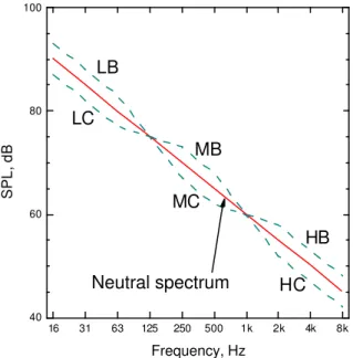
The 15 noise spectra were created by systematically increasing or decreasing the levels in the low, mid and high frequency regions relative to a –5 dB/octave neutral spectrum shape. The concept that a –5 dB/octave spectrum has a neutral quality and the low mid and high frequency groupings were those suggested in the Room Criterion (RC) rating procedure (American Society for Heating Refrigerating and Air Conditioning Engineers (ASHRAE), 2001; Blazier, 1981). According to this procedure the 16, 31 and 63 Hz octave bands are considered low frequencies; the 125, 250 and 500 Hz bands mid-frequencies and the 1000, 2000, and 4000 Hz bands are high frequencies. Figure 2 illustrates conceptually the increases and decreases in these three frequency ranges that were used to create the experimental noise spectra and gives the two-letter names of each noise spectrum increase (boost) or decrease (cut). The 15 noise spectra were created through trial and error, selecting clearly obvious changes resulting from combinations of the various boosts and cuts to the three frequency ranges.

16 31 63 125 250 500 1k 2k 4k 8k 40 60 80 100 HC MC LC Neutral spectrum HB MB LB SPL, dB Frequency, Hz

Figure 2. Symbolic illustration of the noise spectrum shapes used in Experiment 1. LC=low cut, LB=low boost, MC=mid cut, MB=mid boost, HC=high cut, HB=high boost

After the various increases (boost) and decreases (cut) were made in each frequency range, the overall levels were then adjusted so that all spectra had the same overall loudness level. Thus subjects experienced only changes in noise spectrum and not changes in noise level.

The average measured noise spectra in each workstation are illustrated in Figure 3. This Figure compares the measured noise spectra with the measured average speech spectrum and also with a –5 dB/octave reference line. Each of the 15 spectrum plots also includes the spectrum name and the calculated SII (Speech Intelligibility Index) value. For example LC-MB-HB indicates that the spectrum was created as the combination of a low cut (LC) a mid boost (MB) and a high boost (HB). One spectrum is described as neutral and approximately parallels the –5 dB/octave reference line. Another spectrum is labelled Neutral+3 dB and is the same Neutral spectrum shape but increased in level by 3 dB. This was included to help tie in results to the second experiment in which both noise levels and spectrum shape were varied.

Table 2 describes the noise conditions in terms of a variety of acoustic indices, taking into account the number of participants who occupied each workstation. Appendix E describes the various noise

(12)

varied a little (42-47 dB(A)), but the range of the overall loudness levels (LLN) was less than 1 dB (except

for the Neutral + 3 spectrum which was deliberately increased in level). These levels are typical of those commonly experienced in office environments (Broner, 1993; Tang & Wong, 1998; Warnock & Chu, 2002).

(13)

Figure 3. The 15 noise spectra (solid lines) from Experiment 1 compared with the measured speech spectrum

(dashed line) and a –5 dB/octave reference line (dotted).

0 10 20 30 40 50 60 70 Neutral SII = 0.44 SPL, dB LB SII = 0.51 LC SII = 0.39 0 10 20 30 40 50 60 70 MB SII = 0.45 SPL, dB MC SII = 0.43 HB SII = 0.37 0 10 20 30 40 50 60 70 LB-MB SII = 0.50 SPL, dB LB-MC SII = 0.52 LC-MB SII = 0.42 0 10 20 30 40 50 60 70 MC-HB SII = 0.36 SPL, dB LC-HB SII = 0.33 LB-MC-HB SII = 0.46 16 31 63 125 250 500 1k 2 k 4k 8k 0 10 20 30 40 50 60 70 LC-MC-HB SII = 0.31 Frequency, Hz SPL, dB 16 31 63 125 250 500 1k 2k 4k 8k Neutral+3 SII = 0.37 Frequency, Hz 16 31 63 125 250 500 1k 2k 4k 8k LC-MB-HB SII = 0.41 Frequency, Hz

(14)

Table 2. Noise measurements for Experiment 1 conditions, averaged across workstations. (See Appendix E for

explanation of these acoustical measures).

Condition SII AI QAI s16-63 Low(A) High(A) Lo-Hi(A)

Neutral 0.44 0.36 2.81 2.09 42.93 38.76 4.18 LB 0.51 0.43 7.19 2.33 42.44 36.63 5.81 LC 0.39 0.31 1.62 1.84 43.71 40.22 3.49 MB 0.45 0.38 3.76 2.00 45.91 37.49 8.42 MC 0.43 0.35 7.84 2.14 40.40 39.78 0.61 HB 0.37 0.29 5.25 2.06 41.01 41.69 -0.68 LB-MB 0.50 0.43 4.92 2.25 44.53 35.89 8.64 LB-MC 0.52 0.44 10.45 2.33 41.24 36.54 4.70 LC-MB 0.42 0.34 5.46 1.89 46.74 38.50 8.24 MC-HB 0.36 0.28 9.34 2.14 38.64 42.85 -4.22 LC-HB 0.33 0.25 6.63 1.81 41.25 43.05 -1.81 LB-MC-HB 0.46 0.37 9.66 2.41 39.33 39.50 -0.17 LC-MC-HB 0.31 0.23 9.38 1.87 38.66 44.64 -5.97 Neutral+3dB 0.37 0.29 3.21 2.13 45.49 40.95 4.55 LC-MB-HB 0.41 0.33 3.07 1.99 43.55 39.84 3.71

Condition RNC RNCnf RC PNC LLN LN(A) S/N(LL) S/N(A)

Neutral 45.42 42.18 36.57 38.83 64.43 43.98 -3.74 -1.23 LB 53.50 51.56 33.94 46.03 64.95 42.92 -4.26 -0.17 LC 38.23 38.23 37.97 39.57 64.51 45.04 -3.82 -2.30 MB 40.97 39.98 36.57 42.06 65.07 46.02 -4.38 -3.27 MC 48.27 45.13 36.20 40.63 64.26 42.86 -3.56 -0.11 HB 39.99 38.65 38.20 39.94 64.56 44.18 -3.86 -1.44 LB-MB 51.68 49.54 35.14 42.60 65.00 44.52 -4.31 -1.77 LB-MC 53.85 51.99 33.29 46.83 64.97 42.00 -4.27 0.75 LC-MB 41.28 41.28 37.57 42.37 65.12 46.99 -4.43 -4.24 MC-HB 42.53 40.24 38.00 40.77 64.64 44.13 -3.95 -1.39 LC-HB 39.62 39.62 39.20 41.23 64.68 45.09 -3.99 -2.35 LB-MC-HB 51.80 49.25 34.57 43.40 64.62 42.15 -3.93 0.59 LC-MC-HB 41.12 41.12 39.17 42.40 64.91 45.55 -4.21 -2.80 Neutral+3dB 50.29 47.71 38.97 42.23 67.14 46.37 -6.44 -3.63 LC-MB-HB 37.94 37.94 37.97 39.17 64.41 44.76 -3.72 -2.02

The outcome measures encompassed several domains: Demographic variables. Participants were asked to record their age, sex, education, years of work experience (both overall and experience as a temporary office worker), the state of their vision (corrected or not), and hearing.

Cognitive and clerical performance. Although satisfaction was the principal outcome of

interest in these experiments, it was necessary to occupy the participants during their exposure to the noise stimuli. These data will be analysed and reported separately. Environmental noise is known to affect performance of complex cognitive tasks and memory (Banbury & Berry, 1998; Sundstrom, 1987). Complex cognitive tasks are typical of many offices; consequently, these tasks have been chosen to represent the tasks that would be performed in real offices in which masking noise systems were installed.

The memory tasks were word list recognition (in which a participant was shown a list of words on the computer screen at the start of each 15-minute trial, and at the end of the trial was asked to select from a list of words those that were on the original list), recall and recognition of text reading (in which participants read a text about an arbitrary subject, and are subsequently asked a few open-ended and multiple-choice questions about the text), and, grammatical fluency (in which participants are presented

(15)

with a sentence in which there is a grammatical error, which they must identify). These tasks encompass episodic, semantic, and incidental memory processes; some of these are known to be influenced by noise exposure (e.g., episodic memory), and others not (semantic memory) (Banbury & Berry, 1998).

Participants were also presented with a passage printed on paper in which there were randomly placed typographical errors. They were required to re-type the text into the computer, correcting the errors as they typed. The software into which they typed the text required correct data entry, and recorded both speed and accuracy.

Satisfaction. Judgements about overall satisfaction with the work setting and the acoustic environment were assessed using a questionnaire developed for this study (Appendix C). Overall ratings of environmental satisfaction were based on three questions adapted from Sundstrom, Town, Rice, Osborn, and Brill (1994). Specific ratings of the degree of distraction of the noise, perceived privacy under those noise conditions, and satisfaction with the acoustic conditions were asked on 5-point Likert scales; some of these were adapted from Sundstrom, Burt, and Kamp (1980) and Sundstrom, Town, Brown, Forman, & McGee (1982). All questionnaires were presented on the computer screen using questionnaire software developed at NRC (Newsham & Tiller, 1995).

Noise sensitivity. Sensitivity to environmental noise is a personality trait that has been considered to help explain responses. To explore such individual differences we asked participants to complete Weinstein's (1978) noise sensitivity scale (Appendix D). Minor changes in wording were made to bring the phrasing up-to-date.

Workday experiences questionnaire. As a standard practice, we ask participants to report on their experiences during the session using open-ended questions about their beliefs concerning the nature of the study and factors that might have affected them during the day.

The schedule for each testing day is depicted in Table 3. Activities in italics took place in the reception room. Those in plain type occurred in the

experimental facility (IERF).

The participants, scheduled in groups of up to 5 (all male or all female) were asked to arrive at 8:30 a.m. and were greeted by the experimenters. They assembled in the reception area outside the IERF for the initial explanation (based on the information outlined in Appendix A), which was presented on videotape to ensure consistency from one testing day to another, and signed the consent form following a question period. While individuals had their hearing sensitivity tested, the rest of the group waited in the reception room. After all had completed this test, each was assigned a workstation in the IERF, which was theirs for the day.

Computer prompts guided the participants through the experimental session. The session began with a demographic questionnaire, which was followed by a set of satisfaction ratings of the neutral-spectrum masking sound, to provide a baseline, and a series of instructions concerning the tasks in each trial. Then, there were fifteen 15-min periods of noise exposure with concurrent speech, cognitive and clerical tasks, and satisfaction questions, and a final questionnaire about their experiences. The session was punctuated by a 45-min lunch break and a 15-min break in the afternoon, taken in the reception room or in the NRC cafeteria in building M-21, across the road.

(16)

Table 3. Schedule for Testing Day. Activities in italic text took place in the reception room; activities in plain text

took place in the IERF.

Approx. Time Task Duration (min)

8:45 a.m. Arrival, greeting, instructions, consent 15

9:00 a.m. Hearing threshold test (individual testing, approx. 10 min each) 50

10:00 Begin session in IERF - Demographics, task practice 10

Baseline satisfaction questions 5

10:15 6 – 18 min trials (exposures to different masking sounds and speech) 108 During each trial participants completed:

• Word List Presentation - 20 sec

• Reading Text - 2 min

• Grammar Fluency (10 ques.) - 3 min • Reading Comprehension (10 ques.) - 3 min • Text Editing/Typing - 3.5 min

These 4 tasks occurred in 4 orders so that at least one person was doing the editing task at any time (to maintain the same degree of distraction from keyboard noise).

• Word List Recognition - 40 sec

• Environmental Satisfaction (16 items) - 5 min

12:00 Lunch 45

12:45 5 – 18 min exposures to different masking sounds 90

14:15 Break 15

14:30 4 - 18 min exposures to different masking sounds 72

15:45 Workday experiences questionnaire 15

16:15 p.m. Debriefing and farewell 15

With 15 experimental conditions, a Latin Square approach to controlling for order effects was not feasible. Instead, there were six different randomised orders of the 15 sound conditions, one for each day of testing. Six sessions were originally planned, but eight were required to reach the desired sample size. Therefore two of the orders were used twice.

There was also a partial control for the order of presentation of the reading texts and grammar questions; a different order was installed in each of the five workstations occupied by participants. Thus, the content of the tasks and the noise conditions were not confounded (although there was some overlap because of the extra testing days). In addition, within trials there were four orders of the reading,

grammar, and editing tasks (between the word list presentation and recall test), so that at any time at least one person did the editing task and the level of keyboard noise distraction was approximately constant.

2.2 Results

The ratings of satisfaction (Appendix C) consisted of 9 acoustic satisfaction questions rated on 5-point scales, three items rating the characteristics of the noise on 5-point scales (rumble, hiss, and loudness), one 7-point scale rating of self-rated productivity, and one 0-100 sliding scale question concerning the intelligibility of the speech sounds. There were also two open-ended questions, responses to which are discussed below.

The responses to three acoustic satisfaction questions (numbers 5, 6, and 13 in Appendix C) were reverse-scored so that low scores always reflect lower satisfaction, and high scores relate to greater satisfaction. All scales are from 0-4. Several attempts were made to reduce the nine items to a smaller subset of interpretable subscales, but the factor structure was not stable (i.e., the results varied depending on noise conditions being rated). Consequently, it was decided to form one overall rating of acoustic satisfaction for each experimental condition, by averaging the responses to the nine items.

(17)

Thus, there were six dependent variables, which were labelled: Acoustic Satisfaction,

Productivity, Speech Intelligibility, Rumble, Hiss, and Loudness. Table 4 shows the descriptive statistics for the six variables for each of the 15 experimental conditions, and overall.

Table 4. Experiment 1 Descriptive Statistics for Satisfaction Measures.

Condition Statistic Acoustic Satisfaction Productivity Speech Intelligibility

Rumble Hiss Loudness

OVERALL a = .88 Range 0.11 – 3.33 0 – 5 0 – 100 0 – 4 0 – 4 0 - 4 Median 1.67 2 64 1 1 2 Mean (SD) 1.68 (0.70) 2.32 (1.10) 60.14 (28.07) 1.28 (1.05) 1.58 (1.13) 2.14 (0.88) Neutral Range 0.33 – 3.00 0 - 4 9 - 100 0 - 4 0 - 4 1 - 4 Median 1.78 2 51 1 1 2 Mean (SD) 1.74 (0.65) 2.50 (0.96) 58.80 (27.20) 1.18 (1.00) 1.51 (0.92) 2.09 (0.78) LB Range 0.33 - 3.00 0 - 5 10 - 100 0 - 4 0 - 4 1 - 4 Median 1.78 2 77 1 1 2 Mean (SD) 1.66 (0.70) 2.46 (1.31) 71.51 (23.19) 1.31 (0.93) 0.97 (1.01) 1.86 (0.81) LC Range 0.33 – 3.00 0 - 5 0 - 100 0 - 4 0 - 4 1 - 4 Median 1.89 2 67 1 1 2 Mean (SD) 1.71 (0.70) 2.37 (1.17 58.37 (27.63) 1.26 (1.12) 1.57 (1.12) 2.17 (0.86) MB Range 0.33 - 3.11 0 - 5 10 - 95 0 - 4 0 - 4 1 - 4 Median 1.78 3 63 1 1 2 Mean (SD) 1.77 (0.68) 2.60 (1.09) 59.09 (25.68) 1.54 (0.98) 1.23 (0.94) 2.00 (0.80) MC Range 0.33 - 3.11 0 - 4 12 - 100 0 - 4 0 - 4 1 - 4 Median 1.67 2 65 1 1 2 Mean (SD) 1.58 (0.68) 2.11 (1.02) 64.46 (27.94) 1.26 (0.99) 1.46 (1.04) 2.14 (0.88) HB Range 0.33 - 2.89 0 - 5 15 - 100 0 - 4 0 - 4 1 - 4 Median 1.78 2 52 1 2 2 Mean (SD) 1.72 (0.72) 2.41 (0.99) 54.11 (26.34) 1.14 (0.91) 1.91 (1.09) 2.09 (0.89) LB-MB Range 0.11 - 3.33 0 - 5 12 - 99 0 - 4 0 - 4 1 - 4 Median 1.67 2 80 1 1 2 Mean (SD) 1.69 (0.75) 2.11 (1.18) 68.14 (25.28) 1.32 (0.91) 1.03 (1.01) 1.91 (0.78) LB-MC Range 0.56 - 3.11 1 - 5 10 - 100 0 - 3 0 - 3 0 - 3 Median 1.67 2 80 1 1 1 Mean (SD) 1.69 (0.70) 2.46 (1.15) 72.00 (27.67) 1.20 (0.96) 0.74 (0.78) 1.63 (0.84) LC-MB Range 0.56 - 3.11 0 - 4 7 - 99 0 - 4 0 - 4 1 - 4 Median 1.89 2 67 1 1 2 Mean (SD) 1.77 (0.72) 2.23 (0.97) 61.11 (26.63 1.54 (1.17) 1.26 (1.01) 2.03 (0.86) MC-HB Range 0.33 - 2.89 0 - 4 9 - 99 0 - 4 1 - 4 1 - 4 Median 1.67 2 64 1 2 3 Mean (SD) 1.65 (0.64) 2.24 (1.02) 57.71 (26.87) 1.03 (1.10) 2.26 (1.01) 2.43 (0.74)

(18)

LC-HB Range 0.33 - 3.11 0 - 5 1 - 98 0 - 4 1 - 4 1 - 4 Median 1.67 2 66 1 2 2 Mean (SD) 1.67 (0.73) 2.20 (1.02) 57.14 (29.72) 1.23 (1.19) 2.14 (1.06) 2.37 (0.97) LB-MC-HB Range 0.11 - 3.11 0 - 4 17 - 100 0 - 4 0 - 4 1 - 4 Median 1.67 2 80 1 2 2 Mean (SD) 1.58 (0.72) 2.06 (1.04) 68.69 (27.17) 1.29 (0.99) 1.77 (0.97) 2.23 (0.88) LC-MC-HB Range 0.33 - 2.89 0 - 5 2 - 100 0 - 4 0 - 4 1 - 4 Median 1.44 2 50 1 3 3 Mean (SD) 1.52 (0.69) 2.09 (1.15) 52.57 (30.58) 0.83 (1.07) 2.77 (1.29) 2.71 (0.93) Neutral +3dB Range 0.33 – 3.00 0 - 5 1 - 100 0 - 4 0 - 4 1 - 4 Median 1.78 2 44 1 1) 3 Mean (SD) 1.77 (0.67) 2.56 (1.13) 48.29 (29.20) 1.69 (1.11) 1.60 (0.95 2.46 (0.89) LC-MB-HB Range 0.33 - 3.22 0 - 5 0 - 96 0 - 4 0 - 4 1 - 4 Median 1.78 2 57 1 1 2 Mean (SD) 1.70 (0.75) 2.47 (1.19) 50.06 (30.33) 1.31 (1.16) 1.40 (1.03) 2.03 (0.90)

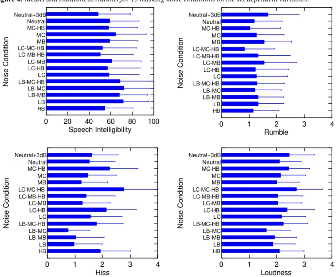
Figure 4 shows the means and standard deviations for the six dependent variables and 15 noise conditions in graphic form. The effects of masking noise spectrum are clearly larger on the ratings of the noise (speech intelligibility, rumble, hiss, and loudness) than on the satisfaction ratings (acoustic satisfaction and self-rated productivity). This is evident from the greater variability in the means. Moreover, none of the satisfaction or productivity means rise above the midpoints of the scales on which they were measured (2 for satisfaction, and 3 for productivity), indicating that on average the participants found none of the noise conditions to be satisfactory.

Figure 4. Means and standard deviations for 15 masking noise conditions on the six dependent variables.

HB LB LB-MB LB-MC LB-MC-HB LC LC-HB LC-MB LC-MB-HB LC-MC-HB MB MC MC-HB Neutral Neutral+3dB Noise Condition 0 1 2 3 4 Acoustic Satisfaction HB LB LB-MB LB-MC LB-MC-HB LC LC-HB LC-MB LC-MB-HB LC-MC-HB MB MC MC-HB Neutral Neutral+3dB Noise Condition 0 2 4 6 Self-Rated Productivity

(19)

Figure 4. Means and standard deviations for 15 masking noise conditions on the six dependent variables. HB LB LB-MB LB-MC LB-MC-HB LC LC-HB LC-MB LC-MB-HB LC-MC-HB MB MC MC-HB Neutral Neutral+3dB Noise Condition 0 20 40 60 80 100 Speech Intelligibility HB LB LB-MB LB-MC LB-MC-HB LC LC-HB LC-MB LC-MB-HB LC-MC-HB MB MC MC-HB Neutral Neutral+3dB Noise Condition 0 1 2 3 4 Rumble HB LB LB-MB LB-MC LB-MC-HB LC LC-HB LC-MB LC-MB-HB LC-MC-HB MB MC MC-HB Neutral Neutral+3dB Noise Condition 0 1 2 3 4 Hiss HB LB LB-MB LB-MC LB-MC-HB LC LC-HB LC-MB LC-MB-HB LC-MC-HB MB MC MC-HB Neutral Neutral+3dB Noise Condition 0 1 2 3 4 Loudness

Prior to proceeding, we performed preliminary statistical tests to determine whether there were overall effects of the noise conditions on the six dependent measures. The omnibus repeated-measures test of Noise Conditions (collapsed across all dependent variables) was statistically significant and

moderate to large in size (F(14, 434) = 5.27, p<.001, partial ?2=.15)*. The interaction test of Dependent

Variable by Noise Condition was also statistically significant ((F(70, 2170) = 6.32, p<.001, partial

?2=.17). The latter test indicates that the effect of the noise conditions differed across the six dependent

variables. We therefore proceeded to examine the exact relationship between the noise conditions and the dependent variables.

Most of the acoustical measures are intended to assess the level of the noise with some particular

*

Partial ?2 is a measure of the strength of the association between the independent and dependent variables (Tabachnick & Fidell, 2001). It is the proportion of variance in the dependent variable that is uniquely attributable to the effect of interest, after all other non-error sources of variance have been removed [Partial ?2 = Sum of

SquaresEFFECT/(Sum of SquaresEFFECT + Sum of SquaresERROR)]. It has a theoretical range from 0 to 1. Because partial ?

2

are based on different denominators, they are not additive (i.e., all the partial ?2 for all the effects on a particular dependent variable can sum to more than 1).

2.2.2 Overall effects of noise conditions.

(20)

weighting of the different frequency components. Only one existing measure (QAI) was found to relate to differences in spectral characteristics. As included in the following section of this report, this was the only acoustical measure found to be significantly related to satisfaction ratings in this experiment. The

importance of particular frequency components of the noise was therefore investigated in more detail. This was done initially in terms of aggregate responses concerning the rating of the rumble, hiss and loudness characteristics of the noises. (Items 2, 3 and 4 in Appendix D). These aggregate response scores were correlated with measured values of octave band noise levels and the resulting correlation coefficients are included in Table 5. Only significant (p < 0.05) results are included.

As expected, mean rumble ratings were most strongly correlated with the 125, 250 and 500 Hz octave band noise levels. (The correlations are negative because these responses were reverse coded). The rumble ratings were also significantly related to some higher frequency noise levels but the sign of the correlation was reversed. Thus although rumble ratings increase with increasing low frequency noise levels, they decrease with increasing high frequency noise levels.

Also as expected, the ratings of the hissy character of the noises were very strongly correlated with the higher frequency octave band noise levels and weakly with the measured noise levels in the 63 and 125 Hz octave bands. Judgements of the loudness of the noises were similarly most strongly correlated with the higher frequency octave band levels because the higher frequencies have a greater influence on loudness.

These results do not agree with the RC rating system (ASHRAE, 2001) that suggests that rumble is related to noise levels in the lowest octave bands (i.e. 16 to 63 Hz). Although the sound levels of the noise spectra in Figure 3 were higher in these very low frequency octave bands, they would not be perceived to be as loud as the 125 to 500 Hz octave band levels. Even though they are representative of typical office noises, some of the lowest octave bands may not even be audible. Thus the 125 to 500 Hz octave band levels probably have greater influence on Rumble ratings because they are more noticeable to subjects.

Table 5. Correlation coefficients for significant (p<0.05) correlations of aggregate ratings of rumble, hiss and loudness and the measured octave band levels of the noises.

Octave noise levels Rumble Hiss Loudness

NL_16 NL_31 NL_63 0.56 NL_125 -0.78 0.55 NL_250 -0.70 NL_500 -0.65 NL_1000 -0.94 -0.88 NL_2000 0.58 -0.95 -0.86 NL_4000 0.59 -0.97 -0.87 NL_8000 0.55 -0.94 -0.88

New measures of the spectral characteristics of the noises were created that included simple approximations to the loudness of the frequency components in various frequency ranges. The loudness estimates were created by weighting the individual octave band noise levels and then summing the A-weighted sound levels over groups of octave bands. In one case the octaves were summed in three groups, as in the RC rating procedure, as low (16 to 63 Hz), mid (125 to 500 Hz) and high (1000 to 4000 Hz) frequency groups. In a simpler scheme only two groups were considered, low (16 to 500 Hz) and high (1000 to 8000 Hz). New spectral measures were then created as differences between the A-weighted levels of the 2 or 3 frequency groups. The simple difference between the A-weighted low (16 to 500 Hz) and high (1000 to 8000 Hz) groups was best correlated with the aggregate ratings of rumble and hiss. This

(21)

level difference between low and high frequency A-weighted levels is referred to as Lo-Hi(A) in this report and was found to be a strong correlate of the aggregate judgements of the rumble (r = 0.859, p< 0.001)and hiss (r = 0.884, p<0.001) characteristics of the noises.

In this experiment, every participant experienced every noise condition. The noise conditions differed slightly depending on which workstation the participant occupied. We can describe the noise conditions as having been nested within individuals. In such a case, hierarchical linear modelling (HLM) is the

appropriate statistical technique to use for predicting dependent variables (acoustic satisfaction, loudness, etc.) from acoustic variables that describe the noise conditions (Bryk & Raudenbush, 1992).

Conceptually, this technique creates separate regression lines for each individual, then tests the slopes of the regression lines for statistical significance against the null hypothesis that the average slope is 0. This separates the variance associated with individuals from the variability associated with the noise conditions, providing a good estimate of the likely population effect.

We selected a subset of 15 different acoustic variables for use in these analyses, all derived from detailed measurements of the acoustic conditions. Although each has its own calculation algorithm, most of the values are highly intercorrelated, which prevented these analyses from using more than one of the variables. We repeated the HLM analyses for the 15 predictors on each of the six dependent variables.

The outcome is summarised in Table 6. The table shows, for each dependent measure, the summary statistics for its prediction from the various acoustic variables. The intercept is the average value (across all 35 participants) that the dependent variable (e.g., acoustic satisfaction) would have if the predictor (e.g., SII) were 0. This value differs widely across individuals and consequently is always statistically significant; further examination of these differences was beyond the scope of this project. The B-weight shown in the table is the average slope of the 35 regression lines (that is, it shows the unit increase in the dependent variable associated with a 1-unit increase in the independent variable). The z

score and associated p and partial ?2 are those associated with the B-weight. ?2partial is the squared partial

correlation coefficient associated with the B-weight for that regression line, and is a measure of effect size, having a theoretical minimum of 0 and maximum of 1 (Tabachnick & Fidell, 2001). This is the unique

variance in acoustic satisfaction explained by that predictor variable. It is calculated as ?2partial =z2/(z2+df)

[for these models, df=34]. The ?2partial values are shown only for those regressions having statistically

significant B-weights.

Table 6. HLM Summary Outcomes

6.A Models for Acoustic Satisfaction

Variable Mean (SD) Min-Max Intercept B-weight zB p ?

2 partial 2.2.4 Predictions from noise characteristics.

(22)

Acoustic Satisfaction 1.68 (0.70) 0.111 - 3.333 - - - - -SII 0.42 (0.07) 0.26-0.56 1.58* 0.211 0.58 0.56 AI 0.34 (0.07) 0.17 - 0.48 1.59* 0.245 0.70 .48 QAI 6.04 (3.06) 0.27-13.19 1.77* -0.016 -2.54 .01 .16 s16-63 2.09 (0.24) 1.64 - 2.69 1.79* -0.052 -0.40 .69 Low(A) 42.39 (2.71) 36.63 - 48.00 ~ ~ ~ ~ High(A) 39.75 (2.57) 34.69 - 45.77 2.14* -0.01 -1.43 .15 Lo-HI(A) 2.63 (4.61) -7.7 - 10.4 1.65* 0.011 3.05 .00 .21 RNC 45.10 (5.76) 37.33-54.91 1.78* -0.002 -0.51 .61 RNCnf 43.63 (5.02) 37.33 - 52.75 1.81* -0.003 -0.51 .56 RC 36.89 (1.97) 32 - 40 1.62* 0.002 0.14 .89 PNC 41.87 (2.42) 37 - 48 1.74* -0.001 -0.16 .87 LLN † 64.89 (0.95) 63.07 - 67.92 ~ ~ ~ ~ LN(A) 44.44 (1.57) 40.37 - 47.84 0.57* 0.025 1.83 .07 S/N(LL) -4.19 (1.36) -8.53 - -2.03 ~ ~ ~ ~ S/N(A) -1.69 (1.81) -5.85 - 2.46 1.64* -0.024 -1.68 .09

Note. *This intercept estimate was statistically significant, reflective of differences in acoustic satisfaction levels

between individuals. ~ This model was unable to be fitted. †In this experiment, LLN was held constant; therefore, it

does not predict any of these outcomes.

6.B. Models for Self-rated Productivity

Variable Mean (SD) Min-Max Intercept B-weight zB p ? 2 partial Self-rated Productivity 2.32 (1.10) 0 - 5 - - - - -SII 0.42 (0.07) 0.26-0.56 2.09* 0.51 0.71 .48 AI 0.34 (0.07) 0.17 - 0.48 2.12* 0.70 0.80 .43 QAI 6.04 (3.06) 0.27-13.19 ~ ~ ~ ~ s16-63 2.09 (0.24) 1.64 - 2.69 2.30* 0.02 0.08 .94 Low(A) 42.39 (2.71) 36.63 - 48.00 ~ ~ ~ ~ High(A) 39.75 (2.57) 34.69 - 45.77 3.21 -0.02 -1.32 .19 Lo-Hi(A) 2.66 (4.62) -7.7 - 10.4 2.27* 0.02 2.51 .01 .16 RNC 45.12 (5.77) 37.33-54.91 2.43* 0.01 -0.32 .75 RNC nf 43.66 (5.02) 37.33 - 52.75 2.46* -0.00 -0.38 .70 RC 36.88 (1.98) 32 - 40 2.44* -0.00 -0.14 .89 PNC 41.89 (2.41) 37 - 48 2.14* 0.00 0.27 .79 LLN † 64.89 (0.95) 63.07 - 67.92 ~ ~ ~ ~ LN(A) 44.45 (1.57) 40.37 - 47.84 1.27* 0.02 1.02 .31 S/N(LL) -4.20 (1.36) -8.53 - -2.03 ~ ~ ~ ~ S/N(A) -1.70 (1.81) -5.85 - 2.46 2.28* -0.03 -1.11 .27

(23)

6.C. Models for Speech Intelligibility

Variable Mean (SD) Min-Max Intercept B-weight zB p ? 2 partial Speech Intelligibility 60.14 (28.07) 0 - 100 - - - - -SII 0.42 (0.07) 0.26-0.56 20.78* 95.61 5.25 .00 .45 AI 0.34 (0.07) 0.17 - 0.48 29.60* 92.09 5.12 .00 .44 QAI 6.04 (3.06) 0.27-13.19 ~ ~ ~ ~ s16-63 2.09 (0.24) 1.64 - 2.69 13.96* 22.42 4.18 .00 .34 Low(A) 42.39 (2.71) 36.63 - 48.00 ~ ~ ~ ~ High(A) 39.75 (2.57) 34.69 - 45.77 139.32 -1.99 -4.60 .00 .38 Lo-Hi(A) 2.63 (4.61) -7.7 - 10.4 58.63* 0.53 2.63 .01 .17 RNC 45.10 (5.76) 37.33-54.91 21.31* 0.86 4.79 .00 .40 RNCnf 43.63 (5.02) 37.33 - 52.75 15.90* 1.01 4.91 .00 .41 RC 36.89 (1.97) 32 - 40 ~ ~ ~ ~ PNC 41.87 (2.42) 37 - 48 -14.20* 1.77 4.29 .00 .35 LLN † 64.89 (0.95) 63.07 - 67.92 ~ ~ ~ ~ LN(A) 44.44 (1.57) 40.37 - 47.84 221.17* -3.62 -5.84 .00 .50 S/N(LL) -4.19 (1.36) -8.53 - -2.03 78.31* 4.30 3.66 .00 .28 S/N(A) -1.69 (1.81) -5.85 - 2.46 66.76* 3.46 5.40 .00 .46

6.D. Models for Rumble Ratings

Variable Mean (SD) Min-Max Intercept B-weight zB p ? 2 partial Rumble 1.28 (1.05) 0 - 4 - - - - -SII 0.42 (0.07) 0.26-0.56 0.83* 1.07 1.54 .12 AI 0.34 (0.07) 0.17 - 0.48 0.88* 1.19 1.78 .08 QAI 6.05 (3.06) 0.27-13.19 ~ ~ ~ ~ s16-63 2.09 (0.24) 1.64 - 2.69 0.99* 0.15 0.65 .51 Low(A) 42.39 (2.71) 36.63 - 48.00 -1.51 0.07 4.29 .00 .35 High(A) 39.75 (2.57) 34.69 - 45.77 3.01 -0.04 -2.60 .01 .17 Lo-Hi(A) 2.63 (4.61) -7.7 - 10.4 1.18* 0.04 4.06 .00 .33 RNC 45.08 (5.77) 37.33-54.91 0.95* 0.01 0.90 .37 RNC nf 43.62 (5.02) 37.33 - 52.75 0.89* 0.01 0.96 .34 RC 36.89 (1.98) 32 - 40 1.85* -0.02 -0.69 .49 PNC 41.88 (2.42) 37 - 48 0.74* 0.01 0.71 .48 LLN † 64.89 (0.96) 63.07 - 67.92 ~ ~ ~ ~ LN(A) 44.44 (1.57) 40.37 - 47.84 -1.12* 0.05 2.03 .04 .11 S/N(LL) -4.19 (1.36) -8.53 - -2.03 0.61* -0.15 -2.76 .01 .18 S/N(A) -1.70 (1.81) -5.85 - 2.46 1.18* -0.05 -2.04 .04 .12

(24)

6.E. Models for Hiss Ratings

Variable Mean (SD) Min-Max Intercept B-weight zB p ? 2 partial Hiss Ratings 1.58 (1.13) 0 - 4 - - - - -SII 0.42 (0.07) 0.26-0.56 4.66* -7.36 -7.80 .00 .64 AI 0.34 (0.07) 0.17 - 0.48 4.09* -7.40 -7.82 .00 .64 QAI 6.04 (3.06) 0.27-13.19 ~ ~ ~ ~ s16-63 2.09 (0.24) 1.64 - 2.69 ~ ~ ~ ~ Low(A) 42.39 (2.71) 36.63 - 48.00 6.70 -0.12 -5.97 .00 .51 High(A) 39.75 (2.57) 34.69 - 45.77 -6.22 0.20 7.99 .00 .65 Lo-Hi(A) 2.63 (4.61) -7.7 - 10.4 1.87* -0.10 -7.43 .00 .62 RNC 45.10 (5.76) 37.33-54.91 ~ ~ ~ ~ RNC nf 43.63 (5.02) 37.33 - 52.75 ~ ~ ~ ~ RC 36.89 (1.97) 32 - 40 ~ ~ ~ ~ PNC 41.87 (2.42) 37 - 48 ~ ~ ~ ~ LLN † 64.89 (0.95) 63.07 - 67.92 ~ ~ ~ ~ LN(A) 44.44 (1.57) 40.37 - 47.84 ~ ~ ~ ~ S/N(LL) -4.19 (1.36) -8.53 - -2.03 ~ ~ ~ ~ S/N(A) -1.69 (1.81) -5.85 - 2.46 ~ ~ ~ ~

6.F. Models for Loudness Ratings

Variable Mean (SD) Min-Max Intercept B-weight zB p ? 2 partial Loudness 2.14 (0.88) 0 - 4 - - - - -SII 0.42 (0.07) 0.26-0.56 3.69* -3.66 -5.64 .00 .48 AI 0.34 (0.07) 0.17 - 0.48 3.38* -3.62 -5.69 .00 .49 QAI 6.05 (3.06) 0.27-13.19 2.11* 0.01 0.64 .52 s16-63 2.09 (0.24) 1.64 - 2.69 3.43* -0.61 -3.86 .00 .31 Low(A) 42.39 (2.71) 36.63 - 48.00 ~ ~ ~ ~ High(A) 39.75 (2.57) 34.69 - 45.77 -1.56 .09 6.10 .00 .52 Lo-Hi(A) 2.63 (4.61) -7.7 - 10.4 2.26* -0.04 -5.58 .00 .48 RNC 45.11 (5.76) 37.33-54.91 2.99* -0.02 -2.84 .01 .19 RNC nf 43.64 (5.01) 37.33 - 52.75 3.12* -0.02 -2.88 .00 .20 RC 36.89 (1.97) 32 - 40 -1.87* 0.11 5.10 .00 .43 PNC 41.88 (2.41) 37 - 48 4.09* -0.05 -3.26 .00 .24 LLN † 64.89 (0.95) 63.07 - 67.92 ~ ~ ~ ~ LN(A) 44.44 (1.57) 40.37 - 47.84 ~ ~ ~ ~ S/N(LL) -4.19 (1.36) -8.53 - -2.03 ~ ~ ~ ~ S/N(A) -1.69 (1.81) -5.85 - 2.46 2.04* -0.06 -2.81 .01 .19

(25)

6.G. Overall HLM Summary.

Variable Signficant Predictions

Significant Predictor of Model Fit Failures

SII 3 Speech Intelligibility, Hiss, Loudness 0

AI 3 Speech Intelligibility, Hiss, Loudness 0

QAI 1 Acoustic Satisfaction 4

s16-63 2 Speech Intelligibility, Loudness 1

Low(A) 2 Rumble, Hiss 4

High(A) 4 Speech Intelligibility, Rumble, Hiss, Loudness 0

Lo-Hi(A) 6 Acoustic Satisfaction, Self-rated Productivity, Speech Intelligibility, Rumble, Hiss, Loudness

0

RNC 2 Speech Intelligibility, Loudness 1

RNC nf 2 Speech Intelligibility, Loudness 1

RC 1 Loudness 2

PNC 2 Speech Intelligibility, Loudness 1

LLN †

0 6

LN(A) 2 Speech Intelligibility, Rumble 2

S/N(LL) 2 Speech Intelligibility, Rumble 4

S/N(A) 3 Speech Intelligibility, Rumble, Loudness 1

The results confirm the initial impression that the noise conditions had a greater effect on the ratings of speech intelligibility and the noise character (rumble, hiss, and loudness) than on the satisfaction and self-rated productivity ratings. More of the acoustic variables were statistically significant predictors, and the effect sizes were larger. This is also not surprising given that most of the acoustic variables were developed as indices of speech intelligibility, the general level of loudness, or the characteristics of the noise.

The complete failure of loudness levels (LLn) to fit a prediction model was of course expected.

This value was held almost constant (within a range of less than 1 dB) across the fifteen noise conditions, with only one condition ("Neutral+3 dB") having a different level. With no variability in this value, it intentionally had no room in which to predict outcomes.

Overall the most consistent predictor was the difference between A-weighted noise levels in low and high frequencies (Lo-Hi(A). It is the only noise characteristic that predicted all six dependent measures; none of the more common measures were as effective. Figure 5 shows the individual trends and the average trend for the six variables, predicted by this value. The left-hand column shows the sets of individual trends, for each hierarchical equation; the right-hand column shows the observed and predicted values and the average regression line. The individual trends show, as one would expect, marked differences between individuals. The average regression lines show that as the Lo-Hi(A) difference increased (i.e., when the loudness of low frequencies exceeded that of high frequencies), acoustic satisfaction, self-rated productivity, and ratings of hiss and loudness all became more favourable. Ratings of rumble increased, but not above the neutral level for the scale (2).

Speech intelligibility became worse (increased slightly) as Lo-Hi(A) increased, which is predictable, because the shift of the balance to more low frequencies (and hence less high frequency noise) would mask speech sounds less well. The slope of the line is small, but statistically significant: speech intelligibility changes by .53 % for a 1 dB(A) increase in the Lo-Hi(A) value (with speech intelligibility scaled from 0 - 100 the line in the graph looks almost flat, even though the effect explains a moderate amount of variance). This result may seem counterintuitive; in that the same acoustic conditions that improved satisfaction tended to lead to greater speech intelligibility and hence less speech privacy. Thus noise that best masks speech sounds and hence leads to greater speech privacy is not necessarily the most acceptable to the subjects. The relationship between acoustic satisfaction, speech intelligibility, and

(26)

hiss ratings is further explored below.

Figure 5. Individual and average trends for dependent variables predicted by Lo-Hi(A)

Individual Trends -10 -5 0 5 10 15 Lo-Hi(A) 0 1 2 3 4 Acoustic Satisfaction ! ! ! ! ! ! ! ! ! ! ! ! ! !! " " " " " " " "" " " " " ## ## #"#" ### # # # # ## Average Trend -10 -5 0 5 10 15 Lo-Hi(A) 0 1 2 3 4 Acoustic Satisfaction Individual Trends -10 -5 0 5 10 15 Lo-Hi(A) 0 2 4 6 SR-Productivity ! ! ! ! ! ! ! ! ! ! ! ! ! !! " " " " " " " "" " " " " ## ## #"#" ### # # # # ## Average Trend -10 -5 0 5 10 15 Lo-Hi(A) 0 2 4 6 SR-Productivity Individual Trends -10 -5 0 5 10 15 Lo-Hi(A) 0 20 40 60 80 100 Speech Intelligibility ! ! ! ! ! ! ! ! ! ! ! ! ! " " " "!"!" _#_{# #}"""" "" _#""" # # # ## # # # # ## Average Trend -10 -5 0 5 10 15 Lo-Hi(A) 0 20 40 60 80 100 Speech Intelligibility

(27)

Figure 5. Individual and average trends for dependent variables predicted by Lo-Hi(A) Individual Trends -10 -5 0 5 10 15 Lo-Hi(A) 0 1 2 3 4 Rumble ! ! ! ! ! ! _! _! _! ! ! ! ! _!_! " " " " " " " " " " " " " " " # # # # # # # # # # # # # # # Average Trend -10 -5 0 5 10 15 Lo-Hi(A) 0 1 2 3 4 Rumble Individual Trends -10 -5 0 5 10 15 Lo-Hi(A) 0 1 2 3 4 Hiss ! ! ! ! ! ! ! ! ! ! ! ! ! ! ! " " " " " " " " " " " " " " " # # # # # # # # # # # # # # # Average Trend -10 -5 0 5 10 15 Lo-Hi(A) 0 1 2 3 4 Hiss Individual Trends -10 -5 0 5 10 15 Lo-Hi(A) 0 1 2 3 4 Loudness !! _! ! ! ! ! ! ! ! _! ! ! ! ! " _" " " " " " " " " _" " " " " # # # # # # # # # # # # # # # Average Trend -10 -5 0 5 10 15 Lo-Hi(A) 0 1 2 3 4 Loudness

. To further explore the relationship between speech intelligibility and hiss ratings in relation to acoustic satisfaction, an HLM model was created with these three variables, in which speech intelligibility and hiss were used to predict acoustic satisfaction. Although the ratings were made simultaneously (as part of one

(28)

questionnaire), this directional relationship makes theoretical sense. The model combining two predictors was possible because ratings of speech intelligibility and hiss were almost uncorrelated (r=.06 over the entire sample and all noise conditions). The results of the HLM analysis are shown in Table 7. It shows that both speech intelligibility and hiss ratings are strong predictors of acoustic satisfaction: reducing speech intelligibility increases acoustic satisfaction, as does reducing hiss.

Table 7. HLM Analyses of acoustic satisfaction in relation to perceived conditions.

Variable Mean (SD) Min-Max Estimate zB p ? 2 partial Acoustic Satisfaction 1.68 (0.70) 0.11 – 3.33 - - - -Intercept 2.42 18.34 .00 Speech Intelligibility 60.14 (28.07) 0 - 100 -0.01 -5.79 .00 .50 Hiss Rating 1.58 (1.13) 0 – 4 -0.12 -5.87 .00 .50 Intercept 1.76 18.61 .00 Rumble 1.28 (1.05) 0 - 4 0.04 -1.43 .15

We also attempted the same analysis with ratings of rumble. The model with both rumble and speech intelligibility failed altogether. A model with rumble alone showed that it was not a significant predictor of acoustic satisfaction (independent of speech intelligibility). The bottom section of Table 7 shows the rumble result.

We hypothesized that individual differences in noise sensitivity might explain overall ratings of environmental satisfaction and ratings of task difficulty at the end of the experiment. Scores on the 21-item Noise Sensitivity Scale (Weinstein, 1978) were regressed on the end-of-day environmental satisfaction ratings and on the average rating of task difficulty (excluding ratings of the difficulty of the hearing test). The results are summarised in Table 8. Neither regression produced a statistically significant result.

Table 8. Regression analyses of Noise Sensitivity (Experiment 1).

Dependent Variable

Predictor

Mean (SD) Cronbach's a Min-Max Estimate t p

ES_End 2.57 (0.82) .88 0.50 - 4.00 Intercept 2.49 NSS 2.50 (0.61) .91 1.48 - 3.62 0.03 0.14 .89 Difficulty 1.75 (0.55) .68 0.50 - 2.83 Intercept 1.38 NSS 2.50 (0.61) .91 1.48 - 3.62 0.15 0.95 .35

Note. All scales have theoretical range from 0 - 4. Lower scores indicate less noise sensitivity (NSS), lower ratings

for task difficulty (Difficulty), and lower ratings for overall environmental satisfaction at the end of the session (ES_End).

2.3 Discussion: Experiment 1

The results of experiment 1 reveal that people are sensitive to changes in the spectral qualities of simulated ambient noise combined with speech when the overall loudness of the noises is not varied. The difference between the A-weighted level of the low frequencies relative to the high frequencies was seen to be related to judgements of the rumble and hiss characteristics of the noises as well a to the overall satisfaction and the speech intelligibility ratings. Louder levels in the low frequencies than high

(29)

frequencies were generally preferred (higher values of Lo-Hi(A)). Higher values of this difference were indicative of more rumbly sounds and lower values of this difference less than 0 dB(A) were rated on the “too hissy” side. The low, mid and high frequency divisions used in the ASHRAE RC rating were not appropriate for explaining judgements of the rumbly character of these noises. Ratings of the rumbly character of the noises were most strongly related to the noise levels in the 125, 250 and 500 Hz octave bands.

Examination of the interrelationships between speech intelligibility and hiss ratings and acoustic satisfaction revealed that conditions that decreased speech intelligibility also increased acoustic

satisfaction. Such conditions generally require more sound energy in the higher frequencies (cf., Table 6.C, which shows a strong relationship between increasing higher frequency noise levels (High(A)) and decreasing speech intelligibility). The challenge, then, lies in establishing the best balance between conditions that reduce speech intelligibility (i.e. increase speech privacy) without decreasing satisfaction with the character of the noise such as caused by increased hiss.

3.0 Experiment 2: Effects of Noise Level and Spectrum

3.1 Method

The second experiment assessed the combined effects of varied noise spectrum and level when combined with speech in situations representative of typical open offices.

All details of the procedures for participant recruitment were the same for experiment 2 as in experiment 1. Data were obtained for 32 participants (38 completed the consent form, but 3 left midway through a session, 2 did not provide valid data, and equipment error invalidated the data from 1 participant). These participants included 15 men and 17 women with age range 19 - 56 years (M=32.7, SD=11.5). Other characteristics are reported in Table 9; the samples for the two experiments are comparable on the variables collected.

Table 9. Characteristics of Experiment 2 Participants.

Hearing Impairment 1 = yes 31 = no Hearing Aid 0 = yes 32 = no Visual Aids 15 = none

10 = distance glasses 3 = bifocals

4 = contact lenses Education 15 = High school

7 = community college / CEGEP 8 = undergraduate degree 2 = graduate degree Years in work force Range 0 year - 37 years

M = 11.9 years SD = 11.3 years

The hearing loss data for Experiment 2 subjects was interpretable. Measured hearing levels relative to threshold values at 500, 1000, 2000, 3000, 4000, and 6000 Hz were summed and subjects with

3.1.1 Objective.

(30)

values greater than 20 were classified as having some hearing impairment. Table 9 indicates that one subject was classified as hearing impaired and data from that subject was excluded from the analyses.

All details of the setting were identical to those for Experiment 1.

The constant speech was identical to that in Experiment 1. There were two independent variables in this experiment, which had a factorial within-subjects experimental design: the noise had five levels (approximately 41, 43, 45, 48, and 51 dB(A)) and the noise spectrum had three levels (LB-MB, neutral, and LC-MB-HB). The three spectra were chosen to provide a range of sound masking potential. The ASHRAE neutral spectrum (ASHRAE, 2001; Blazier, 1981) formed the base case; the Low Boost-Mid Boost (LB-MB) spectrum was chosen to provide an example of stronger low frequency noise (but with lower speech masking), and the Low Cut-Mid Boost- High Boost (LC-MB-HB) spectrum was chosen to provide greater speech masking. Based on the results of Experiment 1, LB-MB would be expected to be more satisfactory than the other conditions, despite its lower speech masking qualities.

The average measured noise spectra in each workstation are illustrated in Figure 6. This figure compares the measured noise spectra with the measured average speech spectrum and also with a –5 dB/octave reference line. Each of the 15 spectrum plots also include the spectrum name and the calculated SII (Speech Intelligibility Index) value. (The spectrum naming convention was explained in section 2.1.3).

Table 10 describes the noise conditions in terms of a variety of acoustic indices, taking into account the number of participants who occupied each workstation. The total noise levels experienced by the participants were between 41 and 51 dB(A), which is within the range of noises found in typical work environments (Broner, 1993; Tang & Wong, 1998).

3.1.3 Setting.

(31)

Figure 6. The 15 noise spectra (solid lines) from Experiment 2 compared with the speech spectrum (dashed line)

and a –5 dB/octave reference line (dotted).

0 10 20 30 40 50 60 70 Neutral-1 SII = 0.52 SPL, dB Neutral-2 SII = 0.47 Neutral-3 SII = 0.40 0 10 20 30 40 50 60 70 Neutral-4 SII = 0.33 SPL, dB Neutral-5 SII = 0.23 LB-MB-1 SII = 0.56 0 10 20 30 40 50 60 70 LB-MB-2 SII = 0.53 SPL, dB LB-MB-3 SII = 0.48 LB-MB-4 SII = 0.42 0 10 20 30 40 50 60 70 LB-MB-5 SII = 0.34 SPL, dB LC-MB-HB-1 SII = 0.50 LC-MB-HB-2 SII = 0.44 16 31 63 125 250 500 1k 2k 4k 8k 0 10 20 30 40 50 60 70 LC-MB-HB-3 SII = 0.37 Frequency, Hz SPL, dB 16 31 63 125 250 500 1k 2k 4k 8k LC-MB-HB-4 SII = 0.29 Frequency, Hz 16 31 63 125 250 500 1k 2k 4k 8k LC-MB-HB-5 SII = 0.20 Frequency, Hz

(32)

Table 10. Noise measurements for Experiment 2 conditions, weighted averages across workstations.

Spectrum Noise Level

SII AI QAI s16-63 Low(A) High(A) Lo-HI(A)

LB-MB 1 0.56 0.48 1.85 2.16 40.90 34.69 6.21 LB-MB 2 0.53 0.45 3.77 2.31 43.23 35.36 7.88 LB-MB 3 0.48 0.40 5.28 2.25 45.85 36.78 9.07 LB-MB 4 0.42 0.34 7.41 2.28 48.73 38.42 10.31 LB-MB 5 0.34 0.28 8.60 2.34 51.62 40.62 11.00 Neutral 1 0.52 0.45 2.46 2.14 39.62 36.27 3.36 Neutral 2 0.47 0.39 2.90 2.12 41.74 37.84 3.89 Neutral 3 0.40 0.33 3.41 2.13 44.15 39.91 4.24 Neutral 4 0.33 0.25 3.90 2.18 46.93 42.27 4.66 Neutral 5 0.24 0.17 4.41 2.10 49.90 44.99 4.90 LC-MB-HB 1 0.50 0.42 5.01 1.89 40.25 36.85 3.40 LC-MB-HB 2 0.44 0.36 4.25 1.98 42.38 38.70 3.67 LC-MB-HB 3 0.37 0.29 4.15 2.08 45.05 40.95 4.10 LC-MB-HB 4 0.29 0.22 3.60 2.10 47.63 43.54 4.10 LC-MB-HB 5 0.20 0.13 3.41 2.09 50.49 46.27 4.22 Spectrum Noise Level RNC RNCnf RC PNC LLN LN(A) S/N(LL) S/N(A) LB-MB 1 44.63 41.45 32.53 37.10 61.62 41.40 -0.74 1.56 LB-MB 2 50.05 46.79 34.10 40.87 63.81 43.35 -2.93 -0.40 LB-MB 3 53.05 51.24 35.67 45.07 66.38 45.77 -5.50 -2.82 LB-MB 4 56.11 54.37 37.67 50.07 69.12 48.48 -8.24 -5.53 LB-MB 5 59.19 57.37 40.67 54.23 71.96 51.29 -11.07 -8.34 Neutral 1 37.42 34.96 33.90 35.63 60.82 41.00 0.06 1.95 Neutral 2 42.50 39.27 35.67 37.37 63.18 42.84 -2.30 0.11 Neutral 3 48.15 44.91 37.67 40.40 65.88 45.09 -4.99 -2.14 Neutral 4 52.08 50.21 40.43 44.83 68.73 47.75 -7.85 -4.79 Neutral 5 54.94 53.41 43.03 49.83 71.80 50.64 -10.92 -7.69 LC-MB-HB 1 34.84 34.84 34.67 36.20 60.89 41.62 -0.01 1.33 LC-MB-HB 2 36.65 36.65 36.67 37.83 63.18 43.58 -2.30 -0.63 LC-MB-HB 3 39.47 39.36 39.03 41.00 65.90 46.12 -5.01 -3.17 LC-MB-HB 4 43.95 42.31 41.67 43.87 68.67 48.67 -7.79 -5.72 LC-MB-HB 5 49.35 46.70 44.43 47.27 71.57 51.47 -10.69 -8.52

The dependent measures were identical to those in Experiment 1.

The procedure was identical to that used in Experiment 1, except that the simulated masking noises were as described in section 3.1.3 above.

3.2 Results

Examination of the dependent variables revealed that one participant had failed to answer the acoustic satisfaction questionnaires for four of the 15 noise conditions. This was judged to be excessive, and data from this participant was excluded from further analyses. Eleven other participants had skipped questions in an apparently random fashion; for these participants, we imputed the means of the available data to be the score. Thus, all data reported here is based on 30 participants.

The dependent variables were the same as in Experiment 1, and are shown for the 15 noise conditions in Table 11 and Figure 7. The graphical presentation reveals that the effects of changing noise

3.1.5 Dependent measures. 3.1.6 Procedure.

(33)

level are likely to be greater than the effects of changing the spectrum of the masking noise. The means for acoustic satisfaction and self-rated productivity never rise above the midpoints of their respective scales, suggesting that none of the sound masking conditions is considered particularly good.

Table 11. Experiment 2 Descriptive Statistics for Satisfaction Measures (N=30)

OVERALL a = .90 Range 0.00 - 3.89 0.00 - 6.00 0.00 - 100.00 0.00 - 4.00 0.00 - 4.00 0.00 - 4.000 Median 1.44 2.00 80.00 1.00 1.00 2.00 Mean (SD) 1.52 (0.80) 2.37 (1.26) 69.10 (31.88) 1.38 (1.08) 1.44 (1.11) 2.06 (0.97) LB-MB -1 Range 0.11 - 3.00 0.00 - 5.00 6.00 - 100.00 0.00 - 2.00 0.00 - 3.00 0.00 - 3.00 Median 1.33 2.00 91.50 1.00 0.00 1.00 Mean (SD) 1.37 (0.76) 2.43 (1.25) 80.70 (28.50) 0.67 (0.71) 0.67 (0.84) 1.37 (0.85) LB-MB-2 Range 0.11 - 2.89 0.00 - 5.00 14.00 - 100.00 0.00 - 3.00 0.00 - 3.00 0.00 - 3.00 Median 1.28 2.00 95.50 1.00 1.00 1.50 Mean (SD) 1.35 (0.78) 2.13 (1.36) 84.70 (21.65) 1.13 (0.78) 0.73 (0.83) 1.53 (0.94) LB-MB-3 Range 0.22 - 2.89 0.00 - 5.00 16.00 - 100.00 0.00 - 3.00 0.00 - 3.00 1.00 - 3.00 Median 1.33 2.00 80.50 1.50 1.00 2.00 Mean (SD) 1.39 (0.69) 2.27 (1.11) 78.43 (24.19) 1.53 (0.68) 1.10 (0.92) 2.03 (0.72) LB-MB-4 Range 0.22 - 3.89 0.00 - 5.00 0.00 - 100.00 1.00 - 4.00 0.00 - 3.00 1.00 - 3.00 Median 1.44 2.00 83.00 2.00 1.00 2.50 Mean (SD) 1.51 (0.81) 2.43 (1.22) 70.53 (31.00) 2.10 (1.09) 1.20 (0.89) 2.40 (0.67) LB-MB-5 Range 0.56 - 3.11 1.00 - 6.00 1.00 - 100.00 0.00 - 4.00 0.00 - 4.00 1.00 - 4.00 Median 1.72 2.00 51.50 2.50 2.00 3.00 Mean (SD) 1.67 (0.77) 2.53 (1.20) 54.70 (31.70) 2.27 (1.11) 1.70 (1.02) 2.57 (0.73) Neutral-1 Range 0.00 - 2.67 0.00 - 6.00 11.00 - 100.00 0.00 - 2.00 0.00 - 2.00 0.00 - 3.00 Median 1.17 2.00 98.50 0.00 0.81 1.00 Mean (SD) 1.16 (0.81) 2.13 (1.57) 87.73 (20.90) 0.53 (0.63) 0.62 (0.67) 1.17 (0.83) Neutral-2 Range 0.22 - 2.67 1.00 - 4.00 21.00 - 100.00 0.00 - 3.00 0.00 - 3.00 1.00 - 3.00 Median 1.41 2.00 89.50 1.00 1.00 2.00 Mean (SD) 1.45 (0.82) 2.35 (1.06) 79.17 (23.41) 1.03 (0.76) 1.10 (0.80) 1.62 (0.61) Neutral-3 Range 0.44 - 3.11 1.00 - 6.00 2.00 - 100.00 0.00 - 2.00 0.00 - 3.00 0.00 - 3.00 Median 1.28 2.00 86.00 1.00 2.00 2.00 Mean (SD) 1.48 (0.73) 2.50 (1.20) 71.73 (33.94) 1.07 (0.69) 1.53 (0.90) 2.10 (0.92) Neutral-4 Range 0.33 - 3.11 1.00 - 6.00 1.00 - 100.00 0.00 - 4.00 0.00 - 4.00 1.00 - 4.00 Median 1.67 2.00 55.00 1.00 2.00 2.50 Mean (SD) 1.75 (0.78 2.53 (1.14) 57.57 (32.67) 1.60 (1.04) 2.07 (0.98) 2.43 (0.82) Neutral-5 Range 0.33 - 3.44 1.00 - 6.00 0.00 - 100.00 0.00 - 4.00 0.00 - 4.00 2.00 - 4.00 Median 1.78 2.34 29.50 2.00 2.50 3.00 Mean (SD) 1.87 (0.90) 2.62 (1.22) 44.57 (35.59) 2.33 (1.03) 2.40 (1.22) 2.90 (0.61) LC-MB-HB-1