Publisher’s version / Version de l'éditeur:
Vous avez des questions? Nous pouvons vous aider. Pour communiquer directement avec un auteur, consultez la première page de la revue dans laquelle son article a été publié afin de trouver ses coordonnées. Si vous n’arrivez pas à les repérer, communiquez avec nous à [email protected].
Questions? Contact the NRC Publications Archive team at
[email protected]. If you wish to email the authors directly, please see the first page of the publication for their contact information.
https://publications-cnrc.canada.ca/fra/droits
L’accès à ce site Web et l’utilisation de son contenu sont assujettis aux conditions présentées dans le site LISEZ CES CONDITIONS ATTENTIVEMENT AVANT D’UTILISER CE SITE WEB.
Student Report; no. SR-2004-08, 2004
READ THESE TERMS AND CONDITIONS CAREFULLY BEFORE USING THIS WEBSITE.
https://nrc-publications.canada.ca/eng/copyright
NRC Publications Archive Record / Notice des Archives des publications du CNRC : https://nrc-publications.canada.ca/eng/view/object/?id=e937bd63-cfee-4d85-8d8d-e3fca2d3c930 https://publications-cnrc.canada.ca/fra/voir/objet/?id=e937bd63-cfee-4d85-8d8d-e3fca2d3c930
NRC Publications Archive
Archives des publications du CNRC
For the publisher’s version, please access the DOI link below./ Pour consulter la version de l’éditeur, utilisez le lien DOI ci-dessous.
https://doi.org/10.4224/8896119
Access and use of this website and the material on it are subject to the Terms and Conditions set forth at Numerical Modeling of a Conventional TEMPSC in Pack Ice
DOCUMENTATION PAGE
REPORT NUMBER
SR-2004-08
NRC REPORT NUMBER DATE
17 December 2004
REPORT SECURITY CLASSIFICATION
Unclassified
DISTRIBUTION
Unlimited
TITLE
Numerical Modeling of a Conventional TEMPSC in Pack Ice
AUTHOR(S)
Bruce W. Quinton
CORPORATE AUTHOR(S)/PERFORMING AGENCY(S)
Institute for Ocean Technology, National Research Council
PUBLICATION
SPONSORING AGENCY(S)
Institute for Ocean Technology, National Research Council
IMD PROJECT NUMBER
PJ00874-PERD
NRC FILE NUMBER
KEY WORDS
Ice-covered waters, lifeboat performance
PAGES 26, App. A-F FIGS. 17 TABLES 7 SUMMARY
This report outlines the numerical modeling of the experimental tests outlined in IOT Publication TR-2003-03. The numerical model is complete and “Fine Tuning” of the ice resistance modeling is currently underway. This report outlines the methods used thus far in “Fine Tuning” and provides documentation for continuation of the work.
It is also recommended that DECICE be upgraded to include bi-linear inter-stiffness capability. This will improve interaction with and between ice elements by modeling the “crushing” that ice undergoes after reaching a certain strain (compression) point.
ADDRESS National Research Council
Institute for Ocean Technology Arctic Avenue, P. O. Box 12093 St. John's, NL A1B 3T5
National Research Council Conseil national de recherches Canada Canada Institute for Ocean Institut des technologies
Technology océaniques
NUMERICAL MODELING OF A CONVENTIONAL TEMPSC IN PACK ICE
SR-2004-08
Bruce W. Quinton
Summary
This report outlines the numerical modeling of the experimental tests outlined in IOT Publication TR-2003-03. The numerical model is complete and “Fine Tuning” of the ice resistance modeling is currently underway. This report outlines the methods used thus far in “Fine Tuning” and provides documentation for continuation of the work.
It is also recommended that DECICE be upgraded to include bi-linear inter-stiffness capability. This will improve interaction with and between ice elements by modeling the “crushing” that ice undergoes after reaching a certain strain (compression) point.
Table of Contents 1.0 INTRODUCTION... 1 2.0 NUMERICAL PHASE ... 2 2.1 DECICE ... 2 2.2 Coordinate System ... 2 2.3 Numerical Model... 3 2.4 Conventional Lifeboat ... 3 2.5 Ice Features... 5
2.5.1 Generating pack ice ... 5
2.5.2 Tess2D outputs ... 6
2.6 Rigid Wall Boundaries ... 6
2.6.1 Creation of the rigid wall boundary model ... 6
2.7 Open Water Area... 6
2.8 Water Resistance ... 7
2.9 Ice Resistance ... 7
3.0 CURRENT STATE OF THE NUMERICAL MODEL ... 8
3.1 Resistance Tests (H Series) ... 8
3.2 Launch Tests (LB Series) ... 9
3.3 Power Type Tests (T Series) ... 10
4.0 FINE TUNING ... 11
4.1 Initial Tests ... 11
4.1.1 Observations and discussion ... 12
4.1.2 General observations ... 13
4.2 Further testing... 13
4.2.1 Observations and discussion ... 14
4.2.2 General observations ... 14
4.3 Inter-stiffness Variance Testing ... 15
4.4 Continuing this Work... 16
5.0 NLBM LAUNCH... 17
5.1 Matlab Simulation ... 18
5.1.2 Coordinate systems used in Matlab ... 18
5.2 MOTION-ELEM Card... 19 5.3 Point in Time... 19 5.4 MOVE-ELEM Card ... 21 5.5 VELOC-DEFN Card... 22 5.6 Discussion ... 23 6.0 CONCLUSION ... 24 7.0 RECOMMENDATIONS ... 24 8.0 REFERENCES... 25
APPENDIX A - TESS2D USER GUIDE ... 3
APPENDIX B - MODEL ICE CONVERSION USER’S GUIDE ... 1
APPENDIX C - INITIAL TEST RESULT PLOTS AND GEOMETRIES ... 1
Appendix C - 1 ... 1
Appendix C - 2 ... 2
Appendix C - 4 ... 4
Appendix C - 5 ... 5
Appendix C - 6 ... 6
APPENDIX D - FURTHER TEST RESULT PLOTS AND GEOMETRIES ... 1
Appendix D – 1 ... 1
Appendix D – 2 ... 2
APPENDIX E – MOVE-ELEM CARD NOTES... 1
APPENDIX F – ANALYZING DECICE HISTORY FILES ... 2
Appendix F-1 - Algorithm for converting DECICE History Files ... 1
Appendix F-2 – Matlab Script for HST_CONV_BQ _V3_2.M ... 1
List of Tables Table 2-1: Hydrostatic and mass properties of conventional lifeboat. ... 4
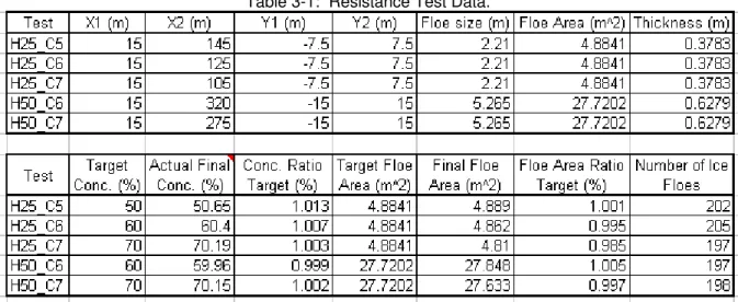
Table 3-1: Resistance Test Data... 8
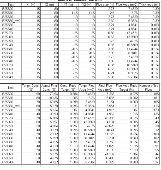
Table 3-2: Launch Test Data... 9
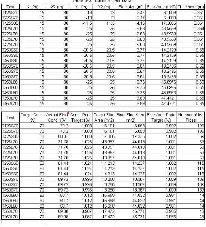
Table 3-3: Launch Test Data... 10
Table 4-1: M13_H50_C7 Test Results. ... 11
Table 4-2: Fine Tuning Test Matrix... 11
Table 4-3: Inter-stiffness variance test matrix... 15
List of Figures Figure 1. DECICE representation of conventional lifeboat hull without canopy... 4
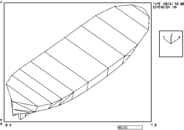
Figure 2. DECICE representation of pack ice... 5
Figure 3. Example Inter-Stiffness vs. Resistance Plot... 15
Figure 4. HYDRO-DAMP Card Equation... 16
Figure 5. System configuration of the Matlab Launch simulation. ... 18
Figure 6. MOTION-ELEM card. ... 19
Figure 7. Graph of lifeboat CG vertical velocity vs. time... 20
Figure 8. Enlargement of graph of z-axis velocity irregularity... 21
Figure 9. Example Bi-linear inter-stiffness... 24
Figure 10. Ice Sheet Area including lower left and upper right coordinate point definitions. ... 3 Figure 11. H50_C7_S1b results. ... 1 Figure 12. H50_C7_S2b results. ... 2 Figure 13. H50_C7_S3b results. ... 3 Figure 14. H50_C7_S4b results. ... 4 Figure 15. H50_C7_S5b results. ... 5 Figure 16. H50_C7_S8b results. ... 1 Figure 17. H50_C7S12b results. ... 2
1.0 INTRODUCTION
In terms of escape-evacuation-rescue, the conclusion of many risk management studies is to fit conventional lifeboats as primary means of evacuation, backed up by rafts.1 An emergency evacuation must be carried out in the environmental conditions that prevail at the time of the emergency.2 Sometimes these environmental conditions include operating in ice-covered waters. The purpose of Phase 1 of this study (PJ00874-PERD) is to discern the effects of pack ice on the performance capabilities of a
conventional TEMPSC (totally enclosed motor propelled survival craft) lifeboat and to define the operating limits of a conventional lifeboat in ice conditions. This project is not a comprehensive evaluation of all aspects of conventional lifeboat performance; rather it is designed to discern the effects of two factors: ice floe concentration and piece size (including thickness). Another purpose is to research the effect of more power on the lifeboat’s performance with respect to these factors. Phase 1 is composed of two portions: the experimental portion and the numerical portion.
The experimental portion of Phase 1 has been completed. This portion included testing a 1:13 scale model of a conventional TEMPSC lifeboat in the ice tank at the National Research Council’s Institute for Ocean Technology (IOT). The following parameters were varied during the tests: pack ice concentration (9/10ths to 5/10ths), ice floe area (small and large), ice floe thickness, and lifeboat powering (required minimum and higher up to 4X). For a complete report and analysis of the experimental portion of Phase 1 see Simões Ré et al (2003).
The numerical portion of Phase 1 consists of trying to duplicate the tests and results from the experimental portion using a full scale numerical simulation created with
DECICE – a numerical modeling program created by INTERA Information Technologies INC., Denver Colorado, and presently owned by Oceanic Corp., St. John’s
Newfoundland.
The previous work term student, Shane Henley, completed some initial work on the numerical simulation that included: the DECICE representation of the numerical lifeboat model (NLBM) (including geometry, hydrostatics, and hydrodynamics), the DECICE representation of the Rigid Wall Boundaries (more precisely a spreadsheet that generates the proper DECICE cards upon user input of desired dimensions), and the open water resistance test simulations. For a complete description the previous numerical simulation work see Lau and Henley (2004).
This report is primarily concerned with documenting the numerical portion of Phase 1.
1
A. Simões Ré, B. Veitch, B. Elliott, S. Mulrooney, Model Testing of an Evacuation System in Ice
Covered Water, TR-2003-03 (Institute for Marine Dynamics 2003), 1. 2
2.0 NUMERICAL PHASE
The numerical phase of this study consists of modeling the necessary physical features of the experimental tests and duplicating the conditions under which the tests were carried out. The numerical model is implemented using DECICE, a program available at the Institute for Ocean Technology (IOT).
2.1 DECICE
DECICE is a numerical modeling program that runs on an Open VMS platform. It is available in two versions: DECICE 2D and DECICE 3D. DECICE3D was used exclusively for the numerical portion of phase 1.
DECICE was developed for analyzing the interaction and fragmentation of discrete and discontinuous media (Lau, 1994) based on a Discrete Element Methodology (DEM). This makes it an ideal solution for modeling ice floe interaction, as individual ice floes can be modeled as discrete elements.
2.2 Coordinate System
The global coordinate system used in the DECICE simulation is located with the x-origin at the aft most point of the initial position of the hull (at t = 0 s) with its positive direction pointing in the direction of the vessel’s initial motion, the z-origin is at waterline elevation with its positive direction pointing vertically upward, and the y-origin is located at the intersection of the x and z axes with its direction governed by the right-hand rule (RHR). The origin of the local coordinate system for the lifeboat model is located at the
element’s centre of gravity (CG) with the positive x-axis pointing toward the bow along the centreline of the vessel, the positive z-axis pointing vertically upward, and the positive y-axis pointing to port (RHR). This local coordinate system moves with the element.
2.3 Numerical Model
The main features of the numerical model are (Lau and Henley, 2004): 1. Numerical Lifeboat Model (NLBM)
2. Pack ice features 3. Rigid wall boundaries 4. Open water area The test conditions include:
• Lifeboat physical parameters • Water physical parameters • Element interaction parameters
In order to differentiate between the different elements, the nodes that define each elements point in space were assigned a starting number: NLBM nodes begin with 3000, rigid wall boundaries begin with a 2000, and ice floe nodes start at 1.
2.4 Conventional Lifeboat
The conventional lifeboat was modeled in DECICE as a motion element (ME). A motion element is a rigid element that is allowed motion in six degrees of freedom. The lifeboat was modeled without the canopy. It was justified as only the hull was expected to have contact with the ice and water and aerodynamic effects on the canopy were negligible for this set of tests.
Figure 1. DECICE representation of conventional lifeboat hull without canopy.
The hydrostatics and mass properties of the conventional lifeboat model used in the physical testing are given in Table 2-1. These values were used to construct the initial version of the DECICE model (Lau and Henley, 2004).
Table 2-1: Hydrostatic and mass properties of conventional lifeboat. Full Scale 1:13 Scale Length Overall (m) 10.0 0.769 Beam at Mid-Ship (m) 3.30 0.259 Displacement (kg) 11800 5.38
Longitudinal Centre of Gravity (m) 4.98 0.383 Vertical Centre of Gravity (m) 1.34 0.103 Draft at Mid-Ship (m) 0.897 0.069
Numerical modeling of the lifeboat required that all the physical model’s properties be accounted for. For the simulation of the lifeboat’s ballast, trim, decay, added mass, and open water resistance characteristics see Lau and Henley’s report (2004).
2.5 Ice Features
The ice floes are simulated using the simply deformable finite elements (SDFE’s) available in DECICE. These elements can be deformed and broken during interaction with their surroundings (i.e. water, rigid wall boundaries, other ice floes, and the
lifeboat). An ice floe that is broken into two pieces becomes two independent elements; thus more accurately describing the role of the ice floes in the simulation. Pack ice floes of specified concentrations, floe areas, and thicknesses were created for analysis.
Figure 2. DECICE representation of pack ice.
2.5.1 Generating pack ice
Pack Ice for the DECICE model test runs were initially generated using Tess2D. Tess2D is a tessellation program that runs on an Open VMS operating system. A tessellation is a group of convex polygons where each polygon is defined by a point that has, as its territory, the area that is closest to it alone. Tess2D asks for an initial
rectangular area (i.e. the dimensions of the ice area), which it reduces to a group of convex polygons such that the sum of the areas of the polygons divided by the initial rectangular area gives the desired concentration of pack ice. Tess2D also requires that the “freeboard” (height above water) and the “ice depth” (depth below waterline) be entered where:
IceDepth Freeboard
ss
IceThickne = + (1)
Other inputs include ice density, number of polygons with greater than 4 sides, tolerances, start piece DECICE element ID, and added mass.
Due to some inherent problems, an iterative process is required to obtain the target output parameters within acceptable error limits. This iterative approach is outlined in Tess2D User Guide – Generating Pack Ice Sheets for use in DECICE Simulations,
which is included in Appendix A. The original documentation for Tess2D is given by Schachter (1993).
2.5.2 Tess2D outputs
Tess2D outputs the pack ice as ME’s – which are modeled as rigid elements. Rigid elements do not represent ice floes very well (especially for the purposes of this study); therefore, they were converted into SDFE’s. Lau and Henley (2004) developed a template to convert the ME’s into SDFE’s. Instructions for converting the ME’s into SDFE’s are included in Appendix B.
2.6 Rigid Wall Boundaries
The rigid wall boundaries are rigid, fixed elements that extend above and below the water surface. Their purpose is to contain the ice floes in the same manner they were restricted in the ice tank during testing. Ideally the rigid wall boundaries should be far enough from the lifeboat-ice and ice-ice interaction to appreciably interfere with the interactions.
2.6.1 Creation of the rigid wall boundary model
Creation of the DECICE rigid wall boundary model was simplified by the creation of a spreadsheet (RIGID BOUNDARIES.XLS) by Lau and Henley (2004). The desired parameters for the rigid wall boundary are input to the spreadsheet and the NODAL-COORD, RIGID-ELEM, and RIGID-CONNEC cards necessary for the DECICE model are output.
2.7 Open Water Area
The open water area allows the lifeboat to attain equilibrium before entering the pack ice. It is also convenient because starting the lifeboat in the pack ice would require making sure the lifeboat would not overlap with the ice floes.
2.8 Water Resistance
The water foundation simulates the effects of water on the boat, the ice, and their interactions). It includes buoyancy and the damping effects of water on the lifeboat. In all cases the water density used was the ice tank water density, 1002.5 kg/m3.
Water effects can be applied by using: • The drag coefficient (CD)
o Applied with the PHYSICAL-CONST card. The drag coefficient applies a universal viscous drag to all elements affected by water except the
lifeboat, which is modeled by a motion element. It is not recommended to use the drag coefficient, as it tends to produce large errors, especially as element velocity increases (Lau and Henley, 2004).
• The HYDRO-DAMP card
o The HYDRO-DAMP card utilizes the six coefficients of a quintic least squares fit of a Surge Resistance vs. Velocity curve and the results of added mass analysis for the remaining five degrees of freedom (Lau and Henley, 2004). This card is applied only to the NLBM.
• The DAMPING-MAT card
o Mass damping can simulate water effects by causing elements to damp the energy transferred to them as if they were in water.
2.9 Ice Resistance
Along with the pack ice generated by Tess2D, element interaction (i.e. ice resistance) must be defined. Ice resistance can be varied by changing the inter-stiffness value of ice-ice, NLBM-ice, and rigid wall boundary-ice interactions. The magnitude of the inter-stiffness affects the level of energy transfer between these elements and therefore the ice resistance.
3.0 CURRENT STATE OF THE NUMERICAL MODEL
Currently “Fine-Tuning” of the numerical model is under way. All the elements of the numerical model are created and implemented, but the element interactions (i.e. the ice resistance) have not been fine-tuned. Once fine-tuning is complete, the model will be ready to simulate the physical tests and results of Phase 1.
Three types of tests are being carried out: resistance tests, launch tests, and power tests. The numerical modeling is complete for all of these tests, with the exception of the “Fine-Tuning”. This means that the NLBM, the rigid wall boundaries, the pack ice sheets, and the water resistance for each numerical test run is completed and compiled into input files to be run in DECICE upon completion of the fine-tuning of the
ice-resistance.
3.1 Resistance Tests (H Series)
The H Series tests are performed to model the lifeboat-ice and ice-ice interactions. To simulate the physical model being attached to the PMM (Planar Motion Mechanism) and being towed down the ice tank, the yaw and sway motions of the lifeboat model are restricted and the NLBM is assigned a constant velocity. This allows measurement of the total resistance on the NLBM.
3.2 Launch Tests (LB Series)
The LB Series tests were designed to simulate the experimental ice tank tests at the minimum required lifeboat power. The NLBM is free to move, and a specified constant thrust force is applied to the model. The NLBM motion is expected to be controlled by the thrust force and the prevailing pack ice condition.
3.3 Power Type Tests (T Series)
The T Series tests were designed to simulate the experimental ice tank tests at greater than the minimum required power level. Again, the NLBM is free to move, and the constant thrust force is increased up to 4 times the original thrust force. Similarly, the NLBM’s motion is expected to be controlled by the thrust force and the prevailing pack ice condition.
4.0 FINE TUNING
As a starting point for fine-tuning the numerical model with respect to NLBM-ice and ice-ice interactions, the ice-ice resistance run M13_H50_C7 from the experiment (Simões Ré et al, 2003) was selected for simulation.
Table 4-1: M13_H50_C7 Test Results.
Model Scale Full Scale
Test Name
Velocity (m/s)Resistance (N)Velocity (m/s)Resistance (N)
0.143 5.12 0.515594 11248.64 0.428 7.773 1.543176 17077.281 0.711 9.549 2.563547* 20979.153* M13_H50_C7 1.137 10.981 4.099512 24125.257 *
Note: these are the target values for the numerical fine-tuning test runs. For fine-tuning the model, the resistance of the ice has to be modified until it reaches the optimal level. Ice resistance is the governing parameter for the velocity of the NLBM. The velocity and ice resistance have to be matched exactly for successful numerical modeling of the experiments.
4.1 Initial Tests
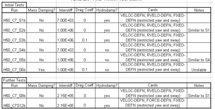
Initially, six test runs were performed varying the above parameters according to the following matrix in Table 4-2. Please note that the NLBM was restricted in yaw and sway motions in all tests.
Table 4-2: Fine Tuning Test Matrix.
*
4.1.1 Observations and discussion
H50_C7_S1b
• The RVELO-DEFN card does not function properly. It fails to have any affect on the post-initial velocity of the NLBM. This is due to the employment of the
HYDRO-DAMP card.
• The VELOC-DEFN card functions properly and is the source of the NLBM’s initial velocity. This velocity eventually goes to zero because there are no positive surge forces acting on the NLBM (i.e. the NLBM slowly stops due to resistance from the pack ice and water).
• The NLBM progressed almost half way along the pack ice sheet and all pack ice floes remained inside the rigid wall boundaries. From observation, this is
assumed to be due to the low 7.00E+03 inter-stiffness value. H50_C7_S2b
• The RVELO-DEFN card does not function properly. It fails to have any affect on the post-initial velocity of the NLBM. This is due to the employment of the
HYDRO-DAMP card.
• The VELOC-DEFN card functions properly and is the source of the NLBM’s initial velocity. This velocity immediately goes to zero because there are no positive surge forces acting on the NLBM (i.e. the NLBM almost immediately stops when it reached the pack ice).
• The NLBM did not progress along the pack ice sheet and initial impact with pack ice floes cause them to disperse outside the rigid wall boundaries. From
observation, this is assumed to be due to the high 1.00E+06 inter-stiffness value. H50_C7_S3b
• The RVELO-DEFN card does not function properly. It fails to have any affect on the post-initial velocity of the NLBM. This is due to the employment of the
HYDRO-DAMP card.
• The VELOC-DEFN card functions properly and is the source of the NLBM’s initial velocity. This velocity immediately goes to zero because there are no positive surge forces acting on the NLBM (i.e. the NLBM almost immediately stops when it reached the pack ice).
• The results were very similar to the results of H50_C7_S2b. At this point in the testing it is not possible to discern the effects of the added CD parameter.
H50_C7_S4b
• The RVELO-DEFN card functions properly and keeps the NLBM at the target velocity (like the physical tow tests). This is because the HYDRO-DAMP card is not employed.
• The VELOC-DEFN card functions properly and is the source of the NLBM’s initial velocity.
• The NLBM progressed to the end of the pack ice sheet and all pack ice floes remained inside the rigid wall boundaries. From observation, this is assumed to be due to the low 7.00E+03 inter-stiffness value.
• The mean surge resistance of approximately 48.8 N is far below the target value of approximately 20,000 N.
H50_C7_S5b
• The RVELO-DEFN card functions properly and keeps the NLBM at the target velocity (like the physical tow tests). This is because the HYDRO-DAMP card is not employed.
• The VELOC-DEFN card functions properly and is the source of the NLBM’s initial velocity.
• The NLBM progressed to the end of the pack ice sheet and most of the pack ice floes dispersed outside the rigid wall boundaries. From observation, this is assumed to be due to the high 1.00E+06 inter-stiffness value.
• The mean surge resistance of approximately 187,000 N is far above the target value of approximately 20,000 N.
H50_C7_S6b
• This run is unstable and will not run to completion. This run attempted to employ mass damping, CD, and the high inter-stiffness value.
4.1.2 General observations
In general, from the first six tests it was noticed that varying the inter-stiff parameter had by far the largest effect on resistance (see plots for H50_C7_S1b and H50_C7_S2b in Appendix C, and notice the difference in order of magnitude of force).
It was also noticed that employment of the HYDRO-DAMP card prevented the RVELO-DEFN card from functioning at all.
4.2 Further testing
Using the approximate maximum resistance from runs H50_C7_S1b and H50_C7_S2b – 1500 N and 90000 N respectfully (each occurred at approximately the same velocity), an inter-stiffness value was interpolated in hopes that it would yield better resistance results. Runs S1b and S2b were chosen because they included the HYDRO-DAMP card, which I wanted to include in the model.
The interpolation used is a standard linear interpolation of a point on a line between two known points, with the following inter-stiffness interpolation equation:
(
)
(
)
(
)
5 3 6 6 1458 . 2 1500 90000 20000 90000 00 . 7 00 . 1 00 . 1 e e e e Interstiff = − − − − = (1)4.2.1 Observations and discussion
H50_C7_S8b
• This run used the interpolated inter-stiffness value. Run H50_C7_S1b was used as a template for this run’s construction.
• Once again the RVELO-DEFN card does not function properly. It fails to have any affect on the post-initial velocity of the NLBM. This is due to the employment of the HYDRO-DAMP card.
• The VELOC-DEFN card functions properly and is the source of the NLBM’s initial velocity. This velocity eventually goes to zero because there are no positive surge forces acting on the NLBM (i.e. the NLBM slowly stops due to resistance from the pack ice and water).
• The maximum surge resistance result of 31,500 N for this run was much closer to the target resistance of approximately 20,000 N.
H50_C7S12b
• This run used the interpolated inter-stiffness value and the FORCE-DEFN card (applying the target resistance (19155 N) in the positive x-direction (surge) at the NLBM’s CG). Run H50_C7_S9b was used as a template for this run’s
construction.
• The VELOC-DEFN card functions properly and is the source of the NLBM’s initial velocity. This velocity increases dramatically in the open water because of the application of the surge force.
• The average surge velocity result is approximately 5.0 m/s for this run and is double the target velocity of 2.56 m/s.
• The final DECICE geometry display (included in Appendix ###) does not show that many ice floes have dispersed outside the rigid wall boundaries. I believe that this is because the NLBM traveled down the tank too fast for them to move significantly. I believe that, given extra time, a large number will eventually end up outside the rigid wall boundaries.
4.2.2 General observations
Again the use of the HYDRO-DAMP card prevented the model from keeping a constant forward velocity. The interpolated inter-stiffness value seems promising.
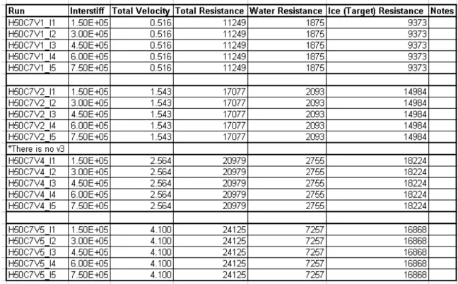
4.3 Inter-stiffness Variance Testing
The interpolated inter-stiffness seems promising and it was decided to pursue further testing of various inter-stiffness values for a given velocity. A series of tests was prepared such that a given velocity was tested with five inter-stiffness values ranging from 1.50E+50 to 3.75E+50 in steps of 1.50E+50. These tests were prepared for the four velocities in Table 4-1.
Table 4-3: Inter-stiffness variance test matrix.
These runs were constructed in hopes of defining a curve (for each velocity) of Inter-stiffness vs. Resistance. Figure 3 shows a hypothetical example of what such a curve might look like. Tests were created for multiple velocities so that inter-stiffness curves for each velocity could be compared to each other in search of similarity. Ideally, they should be approximately equal.
Example Inter-stiffness vs. Resistance Curve for Velocity = Vx1 y = -0.0003x2 + 28.22x + 116119 R2 = 0.9698 0.00E+00 5.00E+05 1.00E+06 0 20000 40000 60000 80000 100000 Resistance Inter-stiffness
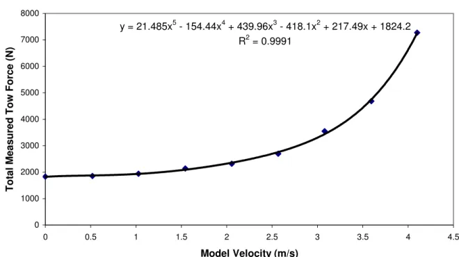
The HYDRO-DAMP card causes the RVELO-DEFN (i.e. constant velocity) card to malfunction; therefore it could not be used in these tests. However, the HYDRO-DAMP card’s function is to calculate and apply the resistance imparted by water at any given velocity. Because, in this case, the velocity in each run is constant, the effects of the HYDRO-DAMP card can be modeled by applying a negative surge force (-Fx) equal to that which the HYDRO-DAMP card would have applied for that velocity. The equation for the HYDRO-DAMP card is shown in Figure 4 and the negative surge force applied in each run is given in the “Water Resistance” column in the above table.
HYDRO-DAMP Card Resistance vs. Surge Velocity
y = 21.485x5 - 154.44x4 + 439.96x3 - 418.1x2 + 217.49x + 1824.2 R2 = 0.9991 0 1000 2000 3000 4000 5000 6000 7000 8000 0 0.5 1 1.5 2 2.5 3 3.5 4 4.5 Model Velocity (m/s)
Total Measured Tow Force (N)
Figure 4. HYDRO-DAMP Card Equation.
4.4 Continuing this Work
Unfortunately, due to time restraint, I was not able to run these tests, and have no further results to report. The procedure necessary to continue this work is outlined here:
1. All 20 test runs for inter-stiff variance have been created and are ready to be run with DECICE. Select a run and execute the simulation using DECICE.
2. Convert the history file produce by DECICE into ASCII data files using “HST_CONV_MLAU.EXE” – a VMS program designed for that purpose. 3. Transfer the “TAPE*.DAT” files produced in Step 2 to a personal computer.
4. Copy “HST_CONV_BQ _V3_2.M” into the directory containing the “TAPE*.DAT” files and then start Matlab.
5. In Matlab, change to the directory containing the files listed in Step 4. Open the “HST_CONV_BQ _V3_2.M” file in a Matlab Editor window and click the “run” button on the toolbar. This will start an interactive analysis program that will allow easy manipulation of the data produced by DECICE. All data will be saved in individual matrices for ease of location and analysis. Refer to HST_CONV_BQ _V3_2.M User’s Guide in Appendix F for a detailed explanation of the options available in this program.
6. Type “y/Y” when prompted to display a plot of Vx and Fx. 7. Type “y/Y” when prompted to produce statistics.
8. Enter “1” when prompted for the number of segments to be analyzed. Be careful not to include data after the point in time that the NLBM has left the pack ice. 9. Click “y/Y” to save the statistics to an ASCII file.
10. Repeat this procedure for each test run.
11. Start an Excel spreadsheet. For each velocity in Table 4-1, enter the mean resistance and inter-stiff value corresponding to each run (five per velocity). 12. For each velocity plot Inter-stiffness vs. Resistance (i.e. make four plots). 13. Find a trendline that provides the best fit for each plot.
14. Compare plots and trendlines, they should be similar.
15. Use the trendlines to find the inter-stiffness value corresponding to the target resistance for each speed in Table 4-1. The inter-stiffness values should be very similar.
16. Enter the inter-stiffness value generated into the Resistance, Launch, and Power tests described above.
5.0 NLBM LAUNCH
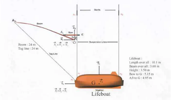
Conventional TEMPSC’s are designed to be launched into the water from the deck of an offshore oil rig or a ship using a flexible boom (see Figure 5). It was desired to perform numerical testing of the launch of the TEMPSC. This section outlines the addition of MOVE-ELEM and VELOC-DEFN cards to the launch numerical model. The objective is to launch a Conventional Lifeboat from 30 metres above the waterline and analyze what happens to it after the launch.
The MOVE-ELEM card was added so that the model element could be placed at the position and orientation corresponding to the point in time just before its bow breaks the water line, after the launch. There was some question as to how the MOVE-ELEM card functions in the numerical simulation. For notes on the use of the MOVE-EMEL card, please see Appendix E.
The VELOC-DEFN card was added so that the model element would have the proper initial velocities (including angular velocity) for the point in time referenced in the MOVE-ELEM card.
5.1 Matlab Simulation
Wayne Raman-Nair previously completed a Matlab model simulation of a Conventional Lifeboat Launch in which the model was raised to 30 metres above the waterline and launched. The data provided by him was in a Matlab file called “MLAUDATA.MAT” and included the position (OG matrix) and velocity (vG matrix) of the lifeboat centre of gravity, angular velocity (omega matrix) of the lifeboat, and orientation of the lifeboat (b1, b2, and b3 matrices – unit vectors representing local x-axis, y-axis, and z-axis directions respectfully, and thetaBoat containing the rotation angles in “Space 3 - 1, 2, 3” format.). All data was provided for a 34 second time period, in tenths of a second time steps (t matrix).
Figure 5. System configuration of the Matlab Launch simulation.
5.1.2 Coordinate systems used in Matlab
The global coordinate system used in the Matlab simulation provided by Wayne Raman-Nair has its origin at the base of the boom, which is 30 metres above the waterline. This simply means that when transferring data to the DECICE simulation, a +30 m offset has to be applied in the global z-direction. For example if the Matlab data has
The local coordinate system used in the Matlab simulation is the same as it is for the DECICE simulation.
5.2 MOTION-ELEM Card
The MOTION-ELEM card included with the numerical model was incomplete and had to be updated. A copy of the correct parameters for the MOTION-ELEM card was
included in Lau and Henley (2004), Appendix B. These parameters were copied and updated (see Figure 6).
Figure 6. MOTION-ELEM card.
5.3 Point in Time
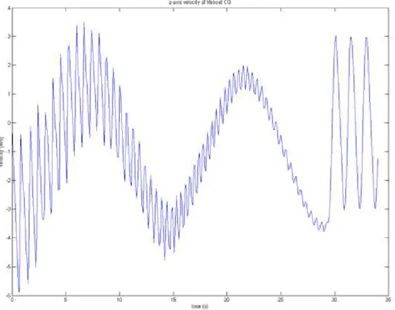
In order to extract the relevant data from the Matlab simulation, the point in time just before the lifeboat’s bow broke the waterline had to be known. To accomplish this the z-axis velocity of the lifeboat’s CG vs. time was plotted and an irregularity was found in the curve that corresponded with the point in time that the lifeboat just entered the water (i.e. a noticeable change in velocity).
Figure 7. Graph of lifeboat CG vertical velocity vs. time.
As can be seen from Figure 7, the irregularity occurs at approximately t = 30 s. An enlargement of this area was then made to determine the precise moment of water entry.
Figure 8. Enlargement of graph of z-axis velocity irregularity.
As you can see from Figure 8 the irregularity occurs at t = 29.3 s. Therefore the relevant data is contained in each matrix at time equal to 29.3 s.
5.4 MOVE-ELEM Card
The MOVE-ELEM card was added so that the model element could be placed at the position and orientation corresponding to the point in time just before its bow breaks the water line, after the launch.
The MOVE-ELEM card needs 21 parameters including:
1. Global element number – There is only the lifeboat which is element 1 => ”1” 2. Global zone number – Not applicable => “0”.
3. Global rotation flag – Flag for using “Space 3 - 1,2,3” rotation algorithm => “1” 4. Local rotation flag – n/a – Flag for using “Body 3 – 1,2,3” rotation algorithm => “0” 5. Global/local scaling flag – n/a => “0”
6. x-component of translation – arbitrary = > “0.00E+00”
7. y-component of translation – arbitrary = 2.9968 m => “0.00E+00” 8. z-component of translation* – See *Note = “1.003303+E00”
10. y-coord of global rotation origin – for “Space 3 – 1,2,3” algorithm => “0.00E+00” 11. z-coord of global rotation origin – for “Space 3 – 1,2,3” algorithm => “0.00E+00” 12. Global angle of rotation about x-axis – thetaBoat_deg(294,1) => “-2.1920E +00” 13. Global angle of rotation about y-axis – thetaBoat_deg(294,2) => “5.5892E -01” 14. Global angle of rotation about z-axis – thetaBoat_deg(294,3) => “1.9899E+01” 15. Local angle of rotation about x-axis – n/a => “0.00E+00”
16. Local angle of rotation about y-axis – n/a => “0.00E+00” 17. Local angle of rotation about z-axis – n/a => “0.00E+00” 18. x-coord of global scaling origin – arbitrary => “0.00E+00” 19. y-coord of global scaling origin – arbitrary => “0.00E+00” 20. z-coord of global scaling origin – arbitrary => “0.00E+00”
21. Scale factor – no scaling (can be 1 or 0 for no scaling) => “1.00E+00”
*Note: The global z-coordinate of translation was found using the following procedure:
1. Rotated the lifeboat to its proper entry position while still submerged in water. 2. Ran the simulation and observed from the DECICE output file, at the initial state
(i.e. time 0.00 s), the global z-coordinate of the lowest node below the water line (i.e. largest negative value).
3. The distance found in 2. is the z-component of translation required to bring the life boat just out of the water.
Therefore the MOVE-ELEM card is: MOVE-ELEM
1 0 1 0 0
0.00E+00 0.00E+00 1.003303E+00
0.00E+00 0.00E+00 0.00E+00
-2.1920E+00 5.5892E-01 1.9899E+01
0.00E+00 0.00E+00 0.00E+00
0.00E+00 0.00E+00 0.00E+00
1.00E+00
5.5 VELOC-DEFN Card
The VELOC-DEFN Card was added to input the initial velocities (both orthographic and angular) of the Conventional Lifeboat just before it enters the water after a launch. This card takes velocities defined in global coordinates, which are taken directly from the vG and omega matrices.
The VELOC-DEFN card requires 11 parameters:
1. Global element number – There is only the lifeboat (element 1) => ”1” 2. Global zone number – Not applicable => “0”.
3. Velocity in global x-direction – vG(294,1) (m/s) => “2.1360E+00” 4. Velocity in global y-direction – vG(294,2) (m/s) => “2.5319E-01”
5. Velocity in global z-direction – vG(294,3) (m/s) => “-3.4487E+00”
6. Angular Velocity about global x-axis – omega(294,1) (rad/s)=>“ -9.4951E-02” 7. Angular Velocity about global y-axis – omega(294,2) (rad/s)=>“ 3.0997E-03” 8. Angular Velocity about global z-axis – omega(294,3) (rad/s)=>“-4.8843E-02” 9. Global x-coordinate of application – See **Note => “0”
10. Global y-coordinate of application – See **Note => “0” 11. Global z-coordinate of application – See **Note => “0” Therefore the VELOC-DEFN card is:
VELOC-DEFN
1 0
2.1360E+00 2.5319E-01 -3.4487E+00
-9.4951E-02 3.0997E-03 -4.8843E-02
0 0 0
**NOTE: DECICE applies the velocities to a user-defined point on the element, but if the global coordinates of application are set to “0”, then DECICE applies the velocities to the centroid of the element by default.
5.6 Discussion
The numerical model of the NLBM launch was successful and is ready to be introduced into other, more involved simulations, including those involving pack ice.
6.0 CONCLUSION
The numerical model for Phase 1 testing is nearly complete. Upon completion of the “Fine Tuning” the model will be ready to reproduce the Phase1 physical tests and results – and will be ready to model future, untested scenarios.
Running the inter-stiffness variance tests and generating the Inter-stiffness vs. Resistance plots should be the major step toward completion of the “Fine Tuning”.
7.0 RECOMMENDATIONS
DECICE does not have the capability to implement bi-linear inter-stiffness values. In some instances, it may be possible for the ice to reach a stress level where it begins to crush. This crushing is associated with an inter-stiffness value that is less than the inter-stiffness associated with ice interaction where crushing is not present. Bi-linear inter-stiffness implementation would significantly improve ice modeling in DECICE.
8.0 REFERENCES
Simões Ré, A., B. Veitch, B. Elliott, and S. Mulrooney. 2003. “Model Testing of An Evacuation System in Ice Covered Water”, IOT Publication: TR-2003-03.
Lau, M., S. Henley. 2004. “DECICE Implementation of Ship Resistance in Ice: Part I – Hydrodynamic Modeling”, IOT Publication: LM-2004-16.
Lau, M. 1994. “A Three-Dimensional “DECICE” Simulation of Ice Sheet Impacting a 90-Degree Conical Structure”, IMD Publication: CR-1994-16.
Tess2D User Guide:
Generating Pack Ice Sheets for use in DECICE Simulations
October 29, 2004
Author: Bruce Quinton
TESS2D USER’S GUIDE – MAKING PACK ICE FOR USE WITH DECICE
Tess2D can be used to produce pack ice sheets for use in simulations run with DECICE.
“Tess2D_AXP.EXE” is the name of the program. It runs on a VMS operating system and requires a terminal window that is open to either MICKEY or PLUTO.
“Tess2D_AXP.EXE” can either be called by a COMMAND file (*.COM) that includes all of the inputs required for Tess2D to create a pack ice sheet, or it can be run directly from a VMS command prompt – in which case the user will be prompted for inputs. Some problems exist within the Tess2D program such that inputs do not become outputs. What this means is that if you are looking for a pack ice sheet that is 6/10 concentration, with an average floe size of 5.0 m2, that is contained within an area defined by (x1, y1) = (15,-10), (x2, y2) = (80, 10) – you will probably end up with a pack ice sheet that is 5/10 concentration, with an average floe size of 4.5 m2, that is
contained within an area defined by (x1, y1) = (15.01,-10.25), (x2, y2) = (79.97, 9.65). Notice that not only are the inputs reduced, but Tess2D also narrows the width of the ice sheet (y2 - y1 should be 20 m but is 19.9 m) and translates the generated ice pieces outside the y1, y2 boundaries (usually only outside y1). This necessitates that the use of Tess2D be a trial and error process with the outputs closely monitored for error. To help with the iterations I have created a helper spreadsheet called “Tess2D Iteration Helper.xls”. The spreadsheet is not for use while running Tess2d it is for use with the outputs from each time Tess2D is run. Its use will be explained throughout the report. I will start with an explanation of running Tess2D from a command prompt to illustrate the inputs that will be required for running it from a COMMAND file.
To start:
1. Set the default directory to the directory you would like the output files to be stored in.
$ SET DEF DISK$PROJECT:[PJ012345.PACK_ICE] or
$ CD DISK$PROJECT:[PJ012345.PACK_ICE]
2. Then start Tess2D from whatever directory it is contained in (e.g. TESS_DIR). $ R DISK$PROJECT:[PJ012345.TESS_DIR]TESS2D_AXP
3. You will be prompted to input the following:
a. Ice sheet area – Tess2D requires that a rectangle be defined by inputting its lower left corner (x1,y1) coordinates and its upper right corner (x2,y2) coordinates. The points (15, -10) and (80, 10) will be used for illustration. These points yield an initial ice sheet area of 1300 m2.
Figure 10. Ice Sheet Area including lower left and upper right coordinate point definitions.
Tess2D asks:
Please enter coordinates for field lower left corner(x,y): 15,-10 Now enter coordinates for field upper right corner(x,y): 80,10 PLEASE NOTE: Tess2D narrows the width (y2 – y1) of the original inputs, therefore the input width may have to be widened (augmented) by 1 or 2 to obtain the target width. For example if you want to create a pack ice sheet that is 50 m wide, you might try (y1, y2) = (-25, 25) and find that the output width is only 48.75 m, you could then try (y1, y2) = 25, 27). If the output is too wide try (-25,26). It is an iterative process.
To find the actual ice sheet width, open the filename.dat file produced by Tess2D in NOTEPAD and copy ONLY the nodal coordinates (i.e. stop at RIGID-ELEM) into the cell A3 on the “Helper” worksheet of “Tess2D Iteration Helper.xls”. You may have to click “Data” → “Text to Columns” → “Deliminated” → “Space Deliminated” if the data appears to be all in the A column. The result will be displayed in the “Actual Ice Sheet Width” cell. You can also enter the target y1 and y2 coordinates in the blue cells provided. Doing so will tell you if all the ice floes are within the target area, and there offset error from the edge of the target area.
PLEASE NOTE: Tess2D translates all the ice floes outside the boundaries you define. By pasting only the NODAL-COORD section of the filename.DAT Tess2D output file in cell A3 of the “Helper” worksheet of “Tess2D Iteration Helper.xls” (see above), and entering the floe “Freeboard” and “Draft” (draft has to be a negative number) in five significant figures in the cells provided, the corrected NODAL-COORD data will be displayed in Yellow on the left-hand side of the worksheet.
b. Pack ice concentration – This is an initial value and will be substantially reduced in the Tess2D output, therefore this value should be inflated. A good start would be to inflate by 10 (i.e. if looking for 6/10 enter 70%).
Enter desired ice concentration: (%) 99.9
PLEASE NOTE: If you widen (augment) the width of the ice sheet in Tess2D to obtain a target final width, the final ice floe concentration (%) will be based on the augmented input area. The actual ice floe concentration will have to be
recalculated. To recalculate, you can open the filename.AREAS output file in NOTEPAD and copy the data into the “Final Ice Floe Concentration” worksheet of “Tess2D Iteration Helper.xls”. You may have to click “Data” → “Text to
Columns” → “Deliminated” → “Space Deliminated” if the data appears to be all in the A column. Then enter the coordinates of the target area in the blue cells provided. The “actual concentration” displayed will be greater than that shown in the Tess2D filename.DAT output.
c. Next you will be given a list of commands followed by a Tess2D command prompt “TESS2D>”.
Commands: q: to quit program.
e: expand the area and generate DECICE input. w: write out points and vertices.
a: add a single point to the current tesselation.
r: add randomly generated points in your defined box. l: list out the neighbor relationships.
p: plot current tesselation. c: clear current tesselation.
Choose “r” allow Tess2D to randomly generate the initial ice floe nodes. TESS2D> r
d. You will now be given a choice to enter the desired number of ice floes in the pack ice sheet or to enter the mean ice floe area (m2). I will proceed with choosing “A” – Enter mean floe Area. As with other user input, this value will be less than entered in the final output. Start with an initial guess that is higher than your target value.
Do you wish to
N. Enter Number of floes, or, A. Enter mean floe Area? a
Mean desired floe area(m^2)? 8.8
Tess2D then echoes an initial guess of the number of floes generated. Initial Number of Floes: 214
e. You will be prompted for an “Integer Seed” input. Tess2D uses this number to “break” the solid ice sheet up and generate ice floes. I
recommend always entering this number as “123”. It is one less variable to worry about and will not affect the outcome greatly.
Integer seed: 123 Creating Points... Inserting Points...
f. You will now be returned to the Tess2D command prompt “TESS2D>”. Commands:
q: to quit program.
e: expand the area and generate DECICE input. w: write out points and vertices.
a: add a single point to the current tesselation.
r: add randomly generated points in your defined box. l: list out the neighbor relationships.
p: plot current tesselation. c: clear current tesselation.
In order to transform the current tessellation into a format DECICE can use, choose the option “E” – expand the area and generate DECICE input.
TESS2D> e
g. You will now be prompted to enter tolerances for "intersection angle” (in degrees), “short side cutoff”( %), and “area cutoff ratio” (%).
Enter tolerence for intersection angle(deg): 20 Enter tolerence for short side cutoff(%): 20 Enter minimum area cutoff ratio(%) 20
h. Tess2D now asks you whether you would like to generate 2D or 3D elements. I will proceed by choosing option “3” to generate 3D rigid elements. NOTE: The spread sheet “Model Ice conversion 2.0.XLS” (S. Henley) is designed to transform these rigid elements into
semi-deformable finite elements. Instructions for the use of this spreadsheet are provided in “Model Ice Conversion User Guide.DOC” (S. Henley).
Would you like
1 2-D Rigid motion elements 2 Non-rigid elastic elements 3 3-D Rigid motion elements Choose 1 or 3; 3
i. You will now be asked to enter the maximum number of ice floes that can have more than four sides.
Enter the maximum possible number of pieces with more than four sides for this problem.
0
j. You will now be asked to enter the filename that the output files (filename.DAT and filename.AREAS) will be saved under.
Please enter the filename areas/cards: RUN_75
k. Tess2D will now echo the final pack ice sheet information. Please note that the final concentration listed here will under estimate the actual concentration if you augmented the width of the ice sheet (y1 and y2) in step a.
Number of Floes: 194 Total Area of Floes: 1495.60 Final Concentration: 79.34
l. You will now be prompted to enter the ice “Freeboard”, which is the height of ice above the water line, followed by “Ice Depth” which is the height of ice below the water line. NOTE: Ice Depth MUST be a negative number if the water line is at elevation=0. An important point to note here is that no matter how many significant figures you input, Tess2D will only output numbers up to 3 decimal places. You can enter the “Freeboard” and “Ice Depth” in the blue cells provided in the “Tess2D Iteration Helper.XLS” spreadsheet. This will replace these parameters in the corrected NODAL-COORD data provided on the left side of the screen.
ss IceThickne Freeboard water ice * 1 ⎥ ⎦ ⎤ ⎢ ⎣ ⎡ − = ρ ρ (1) ss IceThickne Icedepth water ice * ρ ρ = (2)
Enter ice freeboard: 0.047233
Enter ice depth(below datum): -0.34277
m. Next you will be prompted to enter the maximum slope of the ice edge. Enter max. slope of ice edge(deg): 0
n. You will then be prompted to enter the DECICE element number of the first ice floe.
Enter start piece ID: 2
o. You will then be asked for the ice density (ρice).
Enter the mass per unit area of the ice (kg/m^3): 881
p. You will then be asked if you would like to add added mass coefficients for the ice floes. Note: for still ice in calm water there is no initial added mass. DECICE will calculate the added mass for the ice if it moves.
Would you like to enter the added mass coefficients?[N] n
q. Tess2D will then echo some numbers and then display another Tess2D command prompt “TESS2D>”. The tessellation and generation of DECICE output is now complete. You can select ”P” to plot the pack ice sheet or select “Q” to quit the program.
-2.983803 2.983803 -1.000000 -2.397873 2.397874 -0.9999994
-8.134010 8.134015 ...
... 5.445704 -1.000001
-4.242256 4.242261 -0.9999987 Commands:
q: to quit program.
e: expand the area and generate DECICE input. w: write out points and vertices.
a: add a single point to the current tesselation.
r: add randomly generated points in your defined box. l: list out the neighbor relationships.
p: plot current tesselation. c: clear current tesselation.
TESS2D> q
It is possible to automate the above process by creating a COMMAND containing the desired inputs. Doing so facilitates the iteration process of attaining the target outputs. A sample COMMAND file is presented here with comments denoted by “!” preceding them.
This COMMAND file represents the final iteration in generating a pack ice sheet of 7/10 concentration and 43.957 m2 average floe area contained within a 65*50 m2 water surface area.
$ CD DISK$PROJECT:[PJ012345.PACK_ICE] ! set default directory
$ R DISK$PROJECT:[PJ012345.TESS_DIR]TESS2D_AXP ! start Tess2D
15,50 ! (x1,y1) of water surface area (initial offset of 75, y1 suppose to be –25) 80,101 ! (x2, y2) of water surface area (augmentation of +1 (101 - 50 = 50 + 1)) 88.0 ! inflated concentration guess (target = 70%)
r ! choose randomly generated nodal coordinates
a ! choose to input avg. floe area
52.0 ! inflated guess of avg. floe area (target = 43.957)
123 ! integer seed
e ! choose to create DECICE output
20 ! "intersection angle” (in degrees)
20 ! “short side cutoff”(%)
20 ! “area cutoff ratio” (%)
3 ! choose to create 3D rigid element ice floes
0 ! maximum number of pieces with >4 sides
T125L70
0.05098 ! ice freeboard
-0.31302 ! ice depth (draft) (negative if water elevation = 0)
0 ! maximum slope of ice edge in degrees
2 ! DECICE element ID of first ice floe
862 ! ice density (ρice)
n ! choose not to enter added mass coefficients for ice floes
q ! quit Tess2D
PLEASE NOTE: T123L70 is the output file name. Tess2D does not accept comments (i.e. ! comment) after this entry in the COMMAND file.
Model Ice Conversion User’s Guide
Author: S. Henley
Model Ice Conversion User’s Guide
Model Ice conversion is a simple Excel workbook designed to convert the output of the program TESS into a format that is more compatible to DECICE. The steps required to make this conversion are as follows:
• Open the *.DAT file obtained from TESS Using WordPad
• Copy this data into column A of Excel spreadsheet labeled ‘Input’
• Select column A and click Data→Text to Columns, which will open the Convert Text to Columns Wizard:
In step 1, choose Delimited as the Original data type, In step 2, choose the Space Delimiter,
Select Finish
• Scroll down to the beginning of the RIGID-CONNEC command, highlight all of the data until you reach the MOTION-ELEM command, and press copy
Note: only copy the data. Do not copy the Command text or the empty cells • Select cell A3 of the spreadsheet Labeled ‘Conversion 2.0’, and paste the copied
data
• Highlight cells G3 to P3 and drag the Fill Handle (small black square on the lower right corner of highlighted cells) down to the last row of data
Note: This previous step only converts the RIGID-CONNEC code into ELEM-CONNEC for 6-noded wedge elements and 8-noded cuboids.
• Scroll through the newly created code:
If, instead of seeing the word “Code” in column G, you see the word ”12-node”, go to the ‘Formula’ spreadsheet, copy the book-ended cells labeled “12-node only”, and paste the cells into the affected area
If the code in columns I to P display an error, and column J displays the message “10-node”, go to the ‘Formula’ spreadsheet, copy the book-ended cells labeled “10-node only”, and paste the cells into the affected area
Note: 10-noded elements are really just a wedge and a cuboid that share a common face, while 12-noded elements are two cuboids that share a common face
• Once all of the data is verified, go to the spreadsheet labeled ‘ELEM-CONNEC Out’: Select the blue filter arrow next to cell D3
In the menu that appears, select (Custom…)
In the Custom AutoFilter window, the data shown should say “Show rows where ‘2’ is greater than or equal to 0.” Select OK.
This will remove the empty rows that exist in the conversion spreadsheet. This ELEM-CONNEC DECICE code is now ready to be copied into the simulation *.DAT file. If the new code only contains 6 or 8-noded elements, no further steps are necessary. However, if any 10 or 12-noded elements exist, it is required that these elements exist in a locked zone. To create the DECICE code that performs this locking, perform the following:
• For each 10-node and 12-node element, record the nodes that make up that element
• Copy the corresponding nodal geometry data from the NODAL-COORD section of the ‘Input’ spreadsheet, an paste this data into the zero matrix located in the ‘ZONE-DEFN’ spreadsheet
Note: 12 of these zero matrices are already set up for use. If the data requires more, just copy the last matrix/formula cells
• The ZONE-DEFN columns should automatically update with the new code required for DECICE
• Once all of the data is verified, go to the spreadsheet labeled ‘ZONE-DEFN Out’: Select the blue filter arrow next to cell B3
In the menu that appears, select (Custom…)
In the Custom AutoFilter window, the data shown should say “Show rows where ‘1’ does not equal 0.” Select OK.
This will remove the empty rows that exist in the ‘ZONE-DEFN’ spreadsheet. The applicable ZONE-DEFN DECICE code is now ready to be copied into the simulation *.DAT file.
Appendix C - 1
Figure 11. H50_C7_S1b results.
Appendix C - 2
Figure 12. H50_C7_S2b results.
Appendix C - 3
Figure 13. H50_C7_S3b results.
Appendix C - 4
Figure 14. H50_C7_S4b results.
Appendix C - 5
Figure 15. H50_C7_S5b results.
Appendix C - 6 H50_C7_S6b – No Results
Appendix D – 1
Appendix D – 2
Further notes on using the MOVE-ELEM card to apply rotation to an element: Global Rotation
Global rotation is performed about a set of axes parallel to the global axes and located at an origin specified in global coordinates.
The location of the global rotation origin affects only displacement from the global coordinate origin; it has no affect on the final orientation of the element.
The order of global rotation angles is important. DECICE applies rotation about the global x-axis first, followed by rotation about the global y-axis, followed by rotation about the global z-axis. This rule applies to parameters 12, 13, and 14 (global angle of
rotation about n-axis parameters. Local Rotation
Local rotation occurs about a set of axes parallel to the global axes and located at the centre of mass of each element (not the local axis).
The location of the local axes has no effect on element orientation after rotation. The order of local rotation angles is important. DECICE applies rotation about the global x-axis first, followed by rotation about the global y-axis, followed by rotation about the global z-axis. This rule applies to parameters 15, 16, and 17 (global angle of
Appendix F-1 - Algorithm for converting DECICE History Files
This page outlines the procedure necessary for converting DECICE history
(FILENAME.HST) files into a useable Excel Spreadsheet (illustrated with examples). As of version 2 (hst_conv_bq_v2.m), this procedure only works for *.hst files created with the HISTORY-COMBO parameters 1 1 1 1 1 1 1 1 (see additum).
• DECICE history files are corrupted by ftp transfer so they must be analyzed using HST_CONV_MLAU.EXE. To do this:
• from a VMS prompt copy the FILENAME.HST file into the directory containing HST_CONV_MLAU.EXE
$ copy disk$project:[pj042053.test]test.HST disk$project:[pj042053.HST_conv] • then analyze it using HST_CONV_MLAU.EXE, it will prompt you for the
FILENAME, just enter FILENAME without the ending (.HST). $ run HST_CONV_MLAU
Enter history file specification: FILENAME
• This will produce 12 files called TAPE12.DAT, and TAPE 61.DAT to TAPE71.DAT. These files are in ASCII format and are safe for “ASCII transfer” via ftp.
• Transfer the 12 TAPE files to a directory on your computer using whatever method available.
• Copy the hst_conv_bq_v3.m file into the same directory.
• Start Matlab
• Type hst_conv_bq_v3 at the Matlab prompt
> hst_conv_bq_v3
• You can now choose whether to create an Excel Spread in the working directory or not. If you would like to create one, choose a filename, but DO NOT type “.xls” at the end of the filename.
> Please enter the output filename: output
• You can now choose whether to save the Matlab Session or not. If you chose to create an Excel Spreadsheet, the Matlab session will be saved with the same filename (as a *.mat file). If you did not create a spreadsheet, you will be prompted for a filename.
• Please note: if you choose to save either an Excel spreadsheet or the Matlab session, you will not be prompted to enter filenames for other outputs. They will be saved with the same filename.
• You can now choose to plot x-velocity and x-force graphs or not. If you choose ‘n/N’, the program will exit.
• After you plot the graphs, you will be asked whether to generate statistics (min, max, mean) or not. If you choose ‘n/N’, the program exits.
• If you chose to generate statistics, you will be asked to enter an integer
specifying the number of segments you would like to generate statistics for. You can enter this number and then use the mouse to select the start and end times on the graph for each segment. The resulting statistics for each segment will be output on the screen.
• You will now be asked whether you would like to output a file containing the statistics. If you choose ‘n/N’, the program exits. If you choose ‘y/Y’, you may be prompted for a filename. Once again, do not add an extension to the filename as it will be saved as an ASCII “filename.STAT” file.
• If you chose to plot a graph, you will be asked whether you would like to save the graph as a postscript file. If you choose ‘y/Y’, you may be prompted for a
filename and the graph will be saved in the working directory. The program will then exit.
• When the program exits, if you chose to create a spreadsheet, you will see “Warnings” appear but as long as they are not in a red font it is okay. Matlab is just telling you that it is updating the Excel spreadsheet.
Summary
At a VMS prompt analyze the .HST file with HST_CONV_MLAU. Copy the TAPE files to your computer and analyze them again with HST_CONV_BQ in Matlab to produce the Excel spreadsheet and a Matlab session file containing the information in the original DECICE history file. You can also generate statistics for segments and save them in an ASCII *.stat file.
Additum:
The Keyword HISTRY-COMBO determines the data and (their order) output to the *.HST file. For example, if the program is directed to output all 6 available parameters, the order will be as followed:
Input: HISTORY-COMBO 1 1 1 1 1 1 1 Output: Time – tape61(1) Velocity – tape62(1-6)
Strain rate – tape62(7,8) & tape63(1-7) Force – tape63(8) & tape64(1,5)
Space holder ? – tape(7,8) Momentum – tape66(1-6)
Energy (PE,KE,SE,SE(B),TE) – tape66(7,8) & tape67(1-3) Place holder – tape67(4-8) – tape71(1-8)
e.g.
If HISTORY-COMBO is input as: HISTORY-COMBO
1 1 0 0 0 0 1 Then Output is: Time – tape61(1) Velocity – tape62(1-6) Momentum – tape63(1-6)
Energy (PE,KE,SE,SE(B),TE) – tape63(7,8) & tape64(1-3)
This Matlab script is only able to accept data produced by DECICE when the HISTORY-COMBO card is “1 1 1 1 1 1 1”.
Appendix F-2 – Matlab Script for HST_CONV_BQ _V3_2.M
%
================================================================== ======
% This program imports the TAPE files produced by HST_CONV_MLAU.EXE and % exports an Excel spreadsheet and a Matlab session file containing the
% same data. It also allows interactive time segment selection of % x-velocity and x-force for statistics output. A hard copy of these % graphs in .PS format is also an option.
% ================================================================== ====== clear all close all clc % ================================================================== ======
% Get user input --> Make Excel Spreadsheet? %
================================================================== ======
check = 1;
while check == 1
flag1 = input('Would you like to write an .xls file containing this data? (y/n)', 's');
if flag1 == 'y' || flag1 == 'Y'
s = input('Please enter the output filename: ', 's'); fname = strcat(s,'.xls');
check = 2;
elseif flag1 == 'n' || flag1 == 'N' check = 2; else check = 1; end end % ================================================================== ======