Publisher’s version / Version de l'éditeur:
Vous avez des questions? Nous pouvons vous aider. Pour communiquer directement avec un auteur, consultez la première page de la revue dans laquelle son article a été publié afin de trouver ses coordonnées. Si vous n’arrivez pas à les repérer, communiquez avec nous à PublicationsArchive-ArchivesPublications@nrc-cnrc.gc.ca. Questions? Contact the NRC Publications Archive team at
PublicationsArchive-ArchivesPublications@nrc-cnrc.gc.ca. If you wish to email the authors directly, please see the first page of the publication for their contact information.
https://publications-cnrc.canada.ca/fra/droits
L’accès à ce site Web et l’utilisation de son contenu sont assujettis aux conditions présentées dans le site LISEZ CES CONDITIONS ATTENTIVEMENT AVANT D’UTILISER CE SITE WEB.
Proceedings of the International Society for Computers and Their Applications
(ISCA) 14th International Conference on Intelligent and Adaptive Systems and
Software Engineering (IASSE-2005), 2005
READ THESE TERMS AND CONDITIONS CAREFULLY BEFORE USING THIS WEBSITE. https://nrc-publications.canada.ca/eng/copyright
NRC Publications Archive Record / Notice des Archives des publications du CNRC :
https://nrc-publications.canada.ca/eng/view/object/?id=09d77fb1-40ec-459e-a11d-473e39b316aa https://publications-cnrc.canada.ca/fra/voir/objet/?id=09d77fb1-40ec-459e-a11d-473e39b316aa
NRC Publications Archive
Archives des publications du CNRC
This publication could be one of several versions: author’s original, accepted manuscript or the publisher’s version. / La version de cette publication peut être l’une des suivantes : la version prépublication de l’auteur, la version acceptée du manuscrit ou la version de l’éditeur.
Access and use of this website and the material on it are subject to the Terms and Conditions set forth at
A Weighted-Tree Simplicity Algorithm for Similarity Matching of Partial
Product Descriptions
National Research Council Canada Institute for Information Technology Conseil national de recherches Canada Institut de technologie de l'information
A Weighted-Tree Simplicity Algorithm for
Similarity Matching of Partial Product
Descriptions *
Lang, L., Sarker, B.K., Bhavsar, V.C., and Boley, H.
July 2005
* published in the Proceedings of The International Society for Computers and Their Applications (ISCA) 14th International Conference on Intelligent and Adaptive Systems and Software Engineering (IASSE-2005). Toronto, Ontario, Canada. July 20-22, 2005. pp. 55-60. NRC 48534.
Copyright 2005 by
National Research Council of Canada
Permission is granted to quote short excerpts and to reproduce figures and tables from this report, provided that the source of such material is fully acknowledged.
A WEIGHTED-TREE SIMPLICITY ALGORITHM FOR SIMILARITY MATCHING OF
PARTIAL PRODUCT DESCRIPTIONS
Lu Yang Harold Boley
Biplab K. Sarker Institute for Information Technology e-Business Virendrakumar C. Bhavsar National Research Council
Faculty of Computer Science Fredericton, New Brunswick, Canada E3B 9W4 University of New Brunswick harold.boley AT nrc-cnrc.gc.ca
Fredericton, New Brunswick, Canada E3B 5A3 {lu.yang, sarker, bhavsar} AT unb.ca
Abstract
Our weighted-tree similarity algorithm matches buyers and sellers in e-Business environments. We use arc-labeled, arc-weighted trees to represent the products (or services) sought/offered by buyers/sellers. Partial product descriptions can be represented via subtrees missing in either or both of the trees. In order to take into account the effect of a missing subtree on the similarity between two trees, our algorithm uses a (complexity or) simplicity measure. Besides tree size (breadth and depth), arc weights are taken into account by our tree simplicity algorithm. This paper formalizes our buyer/seller trees and analyzes the properties of the implemented tree simplicity measure. We discuss how this measure captures business intuitions, give computational results on the simplicity of balanced k-ary trees, and show that they conform to the theoretical analysis.
Key Words
Arc-labeled and arc-weighted tree, tree similarity, tree simplicity, balanced k-ary trees, e-Business, buyer and seller trees.
1. INTRODUCTION
We proposed earlier a weighted-tree similarity algorithm for multi-agent systems in e-Business environments [1], [8]. In e-Business environments, buyers or sellers seek matching sellers or buyers by exchanging the descriptions of products/services carried by them [3].
Trees are a common data structure for information representation in various areas, such as image comparison, information search and retrieval, clustering, classification, Case-Based Reasoning (CBR) and so on. In e-Business environments, we can also use trees instead of the commonly used key words/phrases to represent the product/service requirements and offers from buyers and sellers. Furthermore, we use node-labeled, arc-labeled and arc-weighted trees to represent parent-child relationship of product/service attributes. Thus, not only node labels but
also arc labels can embody semantic information. The arc weights of our trees express the importance of arcs (product/service attributes). One objective of this paper is to formally define our arc-labeled and arc-weighted trees.
When we compute the similarity of two trees, it is common that a subtree in one tree might be missing in the other one. The similarity of the missing subtree and the empty tree is obtained by computing the simplicity of the missing subtree. An intuitive requirement of the tree simplicity measure is that wider and deeper trees lead to smaller tree simplicity values. However, since our trees are arc-weighted, we also take into account the contribution from arc weights to the tree simplicity. Each arc weight is multiplied with the simplicity value of the recursive subtree simplicity underneath. Hence, another objective of this paper is to analyze and evaluate the mathematical properties of our tree simplicity measure.
In our approach, the tree simplicity values are in the real interval [0, 1]. The simplest tree is a single node whose simplicity is defined as 1.0. Our tree simplicity measure is formalized as a recursive function. According to this function, the simplicity value of an infinite tree approaches 0.0. We conduct experiments on balanced k-ary tree whose arc weights are averaged at each level. The computational results conform to the properties and requirements of our tree simplicity measure.
This paper is organized as follows. Formal definitions of our trees and an overview of our tree similarity algorithm are presented in the following section. In Section 3, we provide the formal descriptions of our tree simplicity measure. Section 4 presents the theoretical and computational results of our tree simplicity measure on balanced k-ary trees. Finally concluding remarks are given in Section 5.
2. ARC-LABELED, ARC-WEIGHTED TREES AND SIMILARITY
In a common e-marketplace, both buyers and sellers advertise their product/service requirements and offers. In order to find matching buyers or sellers, a similarity
computation between them is a must to obtain a ranked similarity list for sellers or buyers. We use arc-labeled and arc-weighted trees to represent product/service requirements and offers. Previous tree similarity (distance) algorithms mostly dealt with trees that have node labels only [4], [5], whether they were ordered [7] or unordered [6]. Due to our unique tree representation for product descriptions, we developed a new weighted-tree similarity algorithm [1], [8]. In this section, we present the definitions of our trees which represent the product/service requirements and offers from buyers and sellers. We also present a brief description of our proposed tree similarity algorithm [1].
2.1 Definitions
Definition 1. Node-labeled trees. A tree T = (V, E, LV) is a 3-tuple where V, E and LV are sets of nodes, arcs and
node labels, respectively, which satisfy the following conditions:
1. One element in V is designated as the 'root'. 2. Each element in E connects a pair of elements in V. 3. There is a unique directed path, consisting of a sequence of elements in E, from the root to each of the other elements in V. 4. There is an (n→1, n ≥1) mapping from the elements in V to the elements in LV (i.e. different nodes can carry the
same labels).
Trees as defined above with only node labels cannot conveniently represent the attributes of products/services, and can lead to ambiguity in some cases.
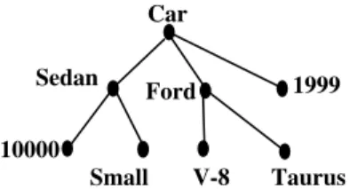
For example, the tree in Figure 1 describes a used car. It is easy to see that this is a small Ford sedan with V-8 engine whose model is Taurus. However, since this is a used car, we cannot figure out what the numbers “1999” and “10000” mean. Although “1999” tends to be the year, it may stand for the price or mileage as well. Similarly, “10000” can also represent the price or mileage of it. Therefore, we add labels to arcs which represent product/service attributes to remove the ambiguity. Figure 2 shows the arc-labeled tree describing the used car shown in Figure 1. We formalize our arc-labeled tree based on Definition 1.
Definition 2. Arc-labeled trees. An arc-labeled tree is a
4-tuple T = (V, E, LV, LE) of a set of nodes V, a set of arcs
E, a set of node labels LV, and a set of arc labels LE such
that (V, E, LV) is a node-labeled tree and there is an (n→1,
n ≥1, fan-out-unique) mapping from the elements in E to the elements in LE (i.e. non-sibling arcs can carry the
same labels).
Car
For algorithmic convenience we always keep arc labels of siblings in lexicographical order. Now suppose the tree in Figure 2 should represent the requirements of a car buyer. This buyer might have special interests in some car attributes. For example, he/she may want a “Ford” i.e. the maker of the car is quite important to him/her but the “Year” is not that important. In order to reveal special preferences indicated by buyers/sellers, we allow them to specify an importance value (arc weight) for each arc. Figure 3 shows the tree with arc weights. According to the corresponding Definition 3, we represent our arc-labeled and arc-weighted tree as follows.
Definition 3. Arc-labeled, weighted trees. An
arc-labeled, arc-weighted tree is a 5-tuple T = (V, E, LV, LE,
LW) of a set of nodes V, a set of arcs E, a set of node
labels LV, a set of arc labels LE and a set of arc weights
LW = [0,1] such that (V, E, LV, LE) is an arc-labeled tree
and there is an (n→1, n ≥1) mapping from the elements in E to the elements in LW (i.e. different arcs can carry the
same weights).
Finally, Definition 4 introduces a user and algorithmic convenience, also illustrated in Figure 3.
Definition 4. Normalized arc-labeled, arc-weighted trees. A normalized arc-labeled, arc-weighted tree is an
arc-labeled, arc-weighted tree T = (V, E, LV, LE, LW)
having a fan-out-weight-normalized (n→1, n ≥1) mapping from the elements in E to the elements in LW, i.e. the
weights of every fan-out add up to 1.0.
Such normalized trees will be assumed throughout for the rest of this paper.
Car Ford Sedan 10000 Small V-8 Taurus 1999
Figure 1. A node-labeled tree (a used car product).
Ford Sedan
10000
Small V-8 Taurus 1999
Figure 2. An arc-labeled tree.
Category Miles Year Make Engine Model Size 0.8 Car Ford Sedan 10000 Small V-8 Taurus 1999
Figure 3. A (normalized) arc-labeled, arc-weighted tree.
Category Year Make Engine Model Size 0.1 0.1 0.7 Miles 0.5 0.5 0.3
2.2 Tree Similarity
Here, we briefly review our proposed tree similarity algorithm [1], [8]. Generally speaking, our algorithm traverses input trees top-down (root-leaf) and then computes their similarity bottom-up. If two non-empty (sub)trees have identical root node labels, their similarity is computed by a recursive top-down (root-leaf) traversal through the subtrees that are accessible on each level via identical arc labels. The recursion is terminated by two (sub)trees (root-leaf) that are leaf nodes, in which case their similarity is 1.0 if their node labels are identical and 0.0 otherwise. Every tree is divided into some subtrees. So, the top-down traversal and bottom-up computation is recursively employed for every pair of subtrees.
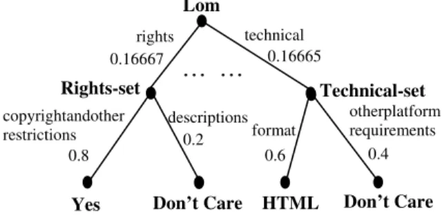
Our algorithm has been incorporated into a subproject of the eduSource project [2]. A goal of this project is to search procurable learning objects for learners. The search results for a learner are represented as a percentage-ranked list of learning objects according to their similarity values with the learner’s query. Figure 4 shows a segment of a learner tree. Another application of the algorithm is our Teclantic portal (http://teclantic.cs.unb.ca) which matches projects according to project profiles represented as trees.
3. TREE SIMPLICITY
During tree similarity computation, when a subtree in tree T1 is missing in tree T2 (or vice versa), we compute
the simplicity of the missing subtree. Our tree simplicity measure takes into account not only the node degree (breadth) at each level and leaf node depth but also the arc weights for the recursive tree simplicity computation. Intuitively, the simpler the single subtree in T1, the larger
its simplicity and thus the larger its similarity to the corresponding empty tree in T2. So, we use the simplicity
as a contribution to the similarity of T1 and T2. Using our
tree simplicity measure, the simplicity converges towards 0.0 when the tree is infinite. However, the simplest tree is a single node and we define that its simplicity is 1.0.
In tree T1 of Figure 5, the subtree rooted at node
“Ford” under the arc “Make” is missing in T2. Our tree
similarity algorithm passes this missing subtree to the treeplicity function to compute its simplicity. Figure 6 shows the pseudo code of this function.
Input: The depth degradation index i. A single tree T. Output: The simplicity value of T.
Initialization: treeplideg = 0.5 //depth degradation factor treeplicity (i ,T)
Begin
If T only contains a single node return i; endif
else
sum=0;
for (j =0; j < root node degree of T; j++); sum+=
(weight of the jth arc) *treeplicity(i*treeplideg, Tj);
//Tj is the subtree under the jth arc
endfor
TreeSimplicity =(1/root node degree of T) * sum;
return TreeSimplicity;
endelse End.
When calling treeplicity with a depth degradation index i and a single tree T as inputs, our simplicity measure is defined recursively to map an arbitrary single tree T to a value from [0, 1], decreasing with both the node degree at each level and leaf node depth. The recursion process terminates when T is a leaf node. For a (sub)tree, simplicity is computed by a recursive top-down traversal through its subtrees. Basically, the simplicity value of T is the sum of the simplicity values of its subtrees multiplied with arc weights from [0, 1], a subtree depth degradation factor ≤ 0.5, and the reciprocal of root node degree of a subtree that is from (0, 1].
For any subtree Tj underneath an arc lj, we multiply
the arc weight of lj withthe recursive simplicity of Tj. To
enforce smaller simplicity for wider trees, the reciprocal of the node degree is used on every level. On each level of deepening, the depth degradation index i is multiplied with a global depth degradation factor treeplideg ≤ 0.5
Lom
Rights-set
Yes Don’t Care HTML
Technical-set rights copyrightandother restrictions technical descriptions format otherplatform requirements Don’t Care 0.16667 0.16665 0.8 0.2 0.6 0.4
… …
Figure 4. Segment of a learner tree.
Figure 6. Pseudo-code of the tree simplicity algorithm.
0.8 Car Ford Sedan 10000 Small V-8 Taurus 1999
Figure 5. Arc-labeled, arc-weighted trees.
Category Miles Yea Car Sedan r Make Engine Model Size 0.1 0.1 0.5 0.5 0.3 0.7 10000 Small 1999 Category Miles Year 0.4 0.6 Size 0.7 0.3 T1 T2
3
and the result is the new value of i in the recursion. We always assume that the value of treeplideg is 0.5.
The smaller the treeplideg factor, the smaller the tree simplicity value. Based on the sum of the infinite
decreasing geometric progression
...
2
1
...
2
1
2
1
2+
+
+
+
n being 1, we assume that treeplideg is 0.5 in order to enforce the smallest acceptable degradation through the recursion: this guarantees that the simplicity values of finite trees are always smaller than 1. For leaf nodes found on any level, the current i value is their simplicity.Our tree simplicity algorithm is given as a recursive function shown below.
(1)
where,
Š(T): the simplicity value of a single tree T
DI and DF: depth degradation index and depth degradation
factor
d: depth of a leaf node
m: root node degree of tree T that is not a leaf
wj: arc weight of the jth arc below the root node of tree T
Tj: subtree below the jth arc with arc weight wj
The initial value of DI represents the simplicity value
of the node with depth 0 (d = 0). Therefore, the simplicity of a tree that is a single node equals to DI. Since an empty
tree is meaningless in our tree simplicity algorithm, we define that the simplicity value of a “single-node” tree is 1.0 which also implies that DI = 1.0. As mentioned before,
the value of DF is defined as 0.5 because of the
employment of decreasing geometric progression.
When a tree horizontally and vertically grows infinitely, the value of m and d will be infinite. Therefore, both (DF)d and 1/m approach 0.0. Since both wj and Š(Tj)
are in the interval [0, 1], equation (1) approaches 0.0 when m and d are infinite.
Now, in order to clarify our tree simplicity algorithm,
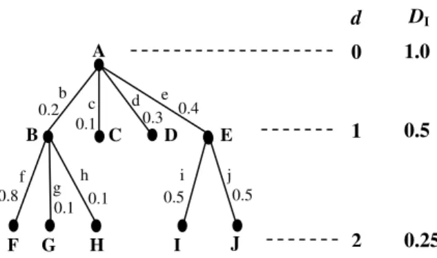
we show the computation of simplicity for an arbitrary tree (Figure 7) with the following illustrative example.
In Figure 7, we show the depth (d) and its corresponding depth degradation index (DI) on the right
hand side of tree T. According to equation (1), the simplicity of this tree is computed as follows.
Š(T) =
4 1
(0.2*Š(TB)+0.1* Š(TB C)+
0.3* Š(TD)+ 0.4* Š(TE)) (3)
In equation (3), the denominator 4 is the degree of the root node of tree T. TB, TB C, TD and TE represent the
subtrees rooted at nodes B, C, D and E respectively. The simplicity values for subtrees (leaf nodes) TC and TD are
their values of DI, 0.5. We recursively use equation (1) for
the simplicity computation of subtrees TBB and TE and get
equations (4) and (5), respectively.
Š(TB) =B 3 1 (0.8*Š(TF)+0.1* Š(TG)+ 0.1* Š(TH)) (4) Š(TE) = 2 1 (0.5*Š(TI)+0.5* Š(TJ)) (5)
Simplicity values for subtrees (leaf nodes) TF, TG, TH,
TI and TJ are their DI value 0.25. Therefore, Š(TB) = B
3 25 . 0 and Š(TE) = 2 25 . 0
. Consequently, we obtain the value of Š(T) 0.06667.
4.ANALYSIS
In this section, we provide the theoretical and computational results to analyze the properties of the proposed tree simplicity measure given in Section 3. For this purpose, we consider balanced k-ary trees, although we do not restrict the degree and depth of each node in the tree. The theoretical results on balanced k-ary tree derived from equation (1) are a non-recursive function with two variables k and d. A k-ary tree is a normalized arc-labeled, arc-weighted tree according to Definition 4 such that the value of m in equation (1) is always a fixed k. The computational results indicate that tree simplicity values smoothly decrease with increasing k and d, which conform to our requirement. Here, both k and d are equal
{
= Š(T) I d D ) ( F D ⋅∑
= ⋅ m T Š w m 1 j j j ( ) 1 if T is a leaf node, otherwise.lim
∞ →→∞ d m Š( T) = 0 (2)Figure 7. An illustrative tree T with d and DI.
A B F b 0.8 0.2 0.5 0.5 C D E c d e f g h i j G H I J 0.1 0.3 0.4 0.1 0.1 1.0 D 0.5 0.25 0 1 2 d I
to or greater than 1. When both of them are equal to 0, the tree is a single node which has been analyzed in Section 3.
In a balanced k-ary tree shown in Figure 8, subtrees under nodes A1 to Ak are shown by triangles since this
tree may have arbitrary depth. All leaf nodes are at the same level; therefore, all leaf nodes have identical depth which is also the tree depth. All arc weights for sibling arcs are averaged. Therefore, we get arc weight 1/k for each arc.
For this special case, equation (1) is simplified as
(6)
where, Tk-ary represents a k-ary tree. After incorporating
the values of DI and DF, we get
(7)
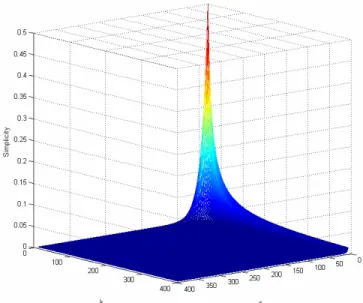
Although equation (2) reveals how the values of m (here, k) and d affect the tree simplicity values, we show the plots for equation (7) to get more intuitive understandings.
Plots generated by Matlab in Figure 9 represent the trend of tree simplicity values for varying d, when k is fixed to 1, 2 and 3. When k is fixed, equation (7) is an exponential function. According to equation (2), the tree simplicity should approach 0.0 when k and d approach infinity. In e-Business/e-Learning environments, it is most likely that trees with very big depth would not arise. For example, in Figure 4, the depth of the given tree is 2. It is evident that we can show the complete tree with this depth for a learner. Therefore, we consider changes to the value of d from 1 to 40 in the subsequent figures. This applies to the value of k as well.
Each plot in Figure 9 has the same trend: tree
simplicity decreases when the depth (d) of the tree increases. However, for the same d, smaller the value of k, bigger is the tree simplicity. Furthermore, bigger the value of k, faster the plot approaches 0.0. This agrees with our analysis of equation (2).
A
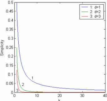
The plots in Figure 10 represent the trend of tree simplicity values for varying k, when the value of d is fixed to 1, 2 and 3. When d is fixed, equation (7) is a polynomial function.
Plots in Figure 10 have trends similar to those in Figure 9. The tree simplicity decreases when the value of k increases. However, for the same k, smaller the value of d, bigger is the tree simplicity. Furthermore, bigger the value of d, faster the plot approaches 0.0.
A1 l l1 k k 1/ 1/ k Ak
Figure 8. A balanced k-ary tree.
Figure 9. Simplicity as a function of d.
I ( D Š( )= 1) ⋅DFd⋅ k Tk−ary d 0 . 1 5 . 0 ) 1 ( ⋅ ⋅ = Š( k−ary) d d k T
Figure 10. Simplicity as a function of k.
The maximum simplicity value for a k-ary tree is 0.5 when both k and d are 1 (1-ary tree). An example tree of this case is shown in Figure 11.
However, both k and d in equation (7) may have arbitrary values. In our computation, we consider every combination when both of them vary from 1 to 40. This means that the maximum root node degree (k) and the maximum depth (d) of the tree are equal to 40. Figure 12 shows the 3-dimensional plot of equation (7). It is easy to find that even when the values of k and d approach 40 (not infinity), the simplicity values are very close to 0.0. This agrees with our requirement that simpler the tree, bigger is the simplicity.
5.CONCLUSION
We have used arc-labeled, arc-weighted trees to represent the product/service descriptions of buyers/ sellers in e-Business/e-Learning environments. We have formalized the definitions of our trees and conducted experiments on balanced k-ary tree. The computational results on this special case agree with our requirement.
Our trees are arbitrary trees without restrictions on node degree and depth. A simpler tree possesses a bigger simplicity value. The simplest tree in our algorithm is a
single node and its simplicity is defined as 1.0. The most complex tree is an infinite tree. The simplicity value for an infinite tree approaches 0.0. We have formalized our tree simplicity measure as a recursive function.
A
B
Figure 11. The k-ary tree when both k and d equal to 1.
a In future, we will further analyze more on the
properties of the general recursive function of our tree simplicity measure and justify our approach not only for k-ary trees.
1.0
ACKNOWLEDGEMENTS
We thank Joseph D. Horton, University of New Brunswick, for discussions about tree definitions and tree simplicity formalizations. We also thank the NSERC for its support through discovery grants of Virendra C. Bhavsar and Harold Boley.
REFERENCES
[1] V. C. Bhavsar, H. Boley and L. Yang, “A weighted-tree similarity algorithm for multi-agent systems in e-business environments,” Computational Intelligence, vol.20, no.4, pp.584-602, 2004.
[2]H. Boley, V. C. Bhavsar, D. Hirtle, A. Singh, Z. Sun and L. Yang, “A match-making system for learners and learning objects,” Learning & Leading with Technology, International Society for Technology in Education, Eugene, Oregon, 2005 (to appear).
[3] A. Chavez and P. Maes, “Kasbah: An agent marketplace for buying and selling goods,” Proceedings of the First International Conference on the Practical Application of Intelligent Agents and Multi-Agent Technology, London, pp.75-90, 1996.
[4] T. Liu and D. Geiger, “Approximate tree matching and shape similarity,” Proceedings of the Seventh International Conference on Computer Vision, Kerkyra, pp.456-462, 1999.
[5] S. Lu, “A tree-to-tree distance and its application to cluster analysis,” IEEE Transactions on Pattern Analysis and Machine Intelligence, PAMI-1(2), pp.219-224, 1979. [6] D. Shasha, J. Wang and K. Zhang, “Exact and approximate algorithm for unordered tree matching,” IEEE Transactions on Systems, Man and Cybernetics, vol.24, no.4, pp.668-678, 1994.
Figure 12. Simplicity as a function of d and k.
[7] J. Wang, B. A. Shapiro, D. Shasha, K. Zhang, and K. M. Currey, “An algorithm for finding the largest approximately common substructures of two trees,” IEEE Transactions on Pattern Analysis and Machine Intelligence, vol.20, pp.889-895, 1998.
[8] L. Yang, M. Ball, V. C. Bhavsar and H. Boley, “Weighted partonomy-taxonomy trees with local similarity measures for semantic buyer-seller matchmaking,” Proceedings of 2005 Workshop on Business Agents and the Semantic Web, Victoria, Canada, pp. 23-35, May 8, 2005.
