Fuzzy synthetic evaluation of disinfection by-products - a risk-based indexing system

Publisher’s version / Version de l'éditeur:

Journal of Environmental Management, 73, 1, pp. 1-13, 2004-10-01

READ THESE TERMS AND CONDITIONS CAREFULLY BEFORE USING THIS WEBSITE.

https://nrc-publications.canada.ca/eng/copyright

Vous avez des questions? Nous pouvons vous aider. Pour communiquer directement avec un auteur, consultez la

première page de la revue dans laquelle son article a été publié afin de trouver ses coordonnées. Si vous n’arrivez pas à les repérer, communiquez avec nous à PublicationsArchive-ArchivesPublications@nrc-cnrc.gc.ca.

Questions? Contact the NRC Publications Archive team at

PublicationsArchive-ArchivesPublications@nrc-cnrc.gc.ca. If you wish to email the authors directly, please see the first page of the publication for their contact information.

NRC Publications Archive

Archives des publications du CNRC

This publication could be one of several versions: author’s original, accepted manuscript or the publisher’s version. / La version de cette publication peut être l’une des suivantes : la version prépublication de l’auteur, la version acceptée du manuscrit ou la version de l’éditeur.

For the publisher’s version, please access the DOI link below./ Pour consulter la version de l’éditeur, utilisez le lien DOI ci-dessous.

https://doi.org/10.1016/j.jenvman.2004.04.014

Access and use of this website and the material on it are subject to the Terms and Conditions set forth at Fuzzy synthetic evaluation of disinfection by-products - a risk-based indexing system

Sadiq, R.; Rodriguez, M. J.

https://publications-cnrc.canada.ca/fra/droits

L’accès à ce site Web et l’utilisation de son contenu sont assujettis aux conditions présentées dans le site LISEZ CES CONDITIONS ATTENTIVEMENT AVANT D’UTILISER CE SITE WEB.

NRC Publications Record / Notice d'Archives des publications de CNRC:

https://nrc-publications.canada.ca/eng/view/object/?id=8ac6f0b3-5a3d-42ad-8892-9f6918ccea72 https://publications-cnrc.canada.ca/fra/voir/objet/?id=8ac6f0b3-5a3d-42ad-8892-9f6918ccea72

Fuzzy synthetic evaluation of disinfection by-products—a risk-based indexing system

Rehan Sadiq and Manuel J. Rodriguez

NRCC-46632

A version of this document is published in / Une version de ce document se trouve dans :

Journal of Environmental Management, Volume 73, Issue 1 , October 2004, pp. 1-13

Fuzzy synthetic evaluation of disinfection by-products – a risk-based

indexing system

1*

Rehan Sadiq and 2Manuel J. Rodriguez

1_{Institute for Research in Construction, National Research Council, Ottawa, ON, Canada, K1A 0R6} 2

Département d’Aménagement, Université Laval, Québec City, QC, Canada, G1K 7P4

Abstract:Disinfection by-products (DBPs) are formed when disinfectants such as chlorine, chloramine, and ozone react with organic matter in water. Chlorine being the most common disinfectant used in the drinking water industry worldwide, significant attention has been focused on chlorinated DBPs. An new indexing method using fuzzy synthetic evaluation is proposed to determine the health risk associated with the two major groups of chlorinated DBPs -

trihalomethanes (THMs) and haloacetic acids (HAAs). Initially, membership functions for cancer and non-cancer risks associated with THMs and HAAs are used to establish the fuzzy evaluation matrices. Subsequently, weighted evaluation matrices for both types of risks are established by performing cross products on the weighted vectors (founded on analytic hierarchy process) and the fuzzy evaluation matrices. In the final stage, the weighted evaluation matrices of cancer and non-cancer risks are aggregated to determine the final risk rating. Two case studies are provided to demonstrate the application of this method.

Keywords: Water quality, DBPs, fuzzy synthetic evaluation, AHP, cancer and non-cancer risk. *Corresponding author

1. INTRODUCTION

The disinfection is performed to eradicate and/or inactivate the pathogens from drinking water. The disinfection involves destruction of organization of cell structure, and interference with energy yielding metabolisms, biosynthesis and growth of microbes. Chlorine and its compounds are the most commonly used disinfectants for water treatment. Chlorine has a very strong oxidizing potential, which provides a residual throughout the distribution system and protects against microbial recontamination.

The addition of disinfecting chemicals to drinking water can reduce the microbial risk but poses chemical risk due to the formation of disinfection by-products (DBPs). Formation of DBPs occurs when the disinfectant reacts with natural organic matter and/or inorganic substances present in water. More than 600 DBPs have been identified in the laboratory scale studies for different disinfectants, while approximately 250 have been identified in drinking water samples taken from actual distribution systems. Among DBPs found in chlorinated drinking water, trihalomethanes (THMs) and haloacetic acids (HAAs) have been the focus of particular attention because of the potential carcinogenicity and harmful non-cancer effects. THMs include four compounds – chloroform (TCM), dichlorobromomethane (DCBM), dibromochloromethane (DBCM) and bromoform (TBM). In waters of low bromide levels, TCM is a major culprit among THMs. HAAs include nine compounds but the most common are – monochloroacetic acid (MCAA), dichloroacetic acid (DCAA), trichloroacetic acid (TCAA), monobromoacetic acid (MBAA), dibromoacetic acid (DBAA), and bromochloroacetic acid (BCAA) (Serodes et al., 2003). Among them, generally DCAA and TCAA are of significant levels in chlorinated drinking water.

The major objective of this research is to develop a risk-based indexing system for chlorinated DBPs found in drinking water using fuzzy synthetic evaluation (FSE) technique. The paper addresses three major issues: identifying toxicity criteria for of DBPs, developing an indexing system by grouping DBPs based on associated adverse health effects, and

1.1. TOXICITY OF THMS AND HAAS

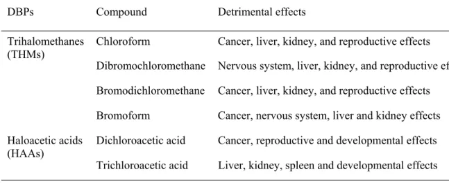
The Safe Drinking Water Act requires the United States Environmental Protection Agency (US EPA) to develop new drinking water regulations. The regulations related to DBPs are part of the Microbial-Disinfection by-products (M-DBPs) rule (US EPA, 1999). The DBP regulations are based on evidence of their potential adverse human health effects, in particular cancer and reproductive disorders (Cantor et al., 1998; Graves et al., 2002). Routine water quality sampling help in identifying whether regulatory thresholds (guideline or standard) of DBPs are violated or not. The threshold values are based on potential toxicity of DBP indicators. A wealth of literature reporting adverse health effects through toxicological laboratory studies is available. Some of the adverse health effects of THMs and few HAAs are summarised in

Table 1.

The World health Organization (WHO, 1993) published drinking water guidelines for a few common DBPs including THMs and HAAs. In addition to guidelines for THMs, the WHO has also suggested that the sum of the ratios of the THM levels to the guideline values should not

exceed 1 (see Table 2). Such guidelines have no official recognition in the US or Canada. The

US EPA (2001) has established the maximum allowable contaminant level of 0.08 mg/L for total THMs and of 0.06 mg/L for HAA5 (the sum of five HAAs, that is mono-, di-, and trichloroacetic

acids and mono- and dibromoacetic acids), respectively. Compliance of these by-products is based on an annual running average of quarterly samples, and since 2002 will also be based on a locational running average (Sharfenaker, 2001). Health Canada (2001) has set total THM levels of 0.10 mg/L as an interim maximum acceptable concentration, which serves as a guideline for Provincial regulations. No Canadian drinking water quality guideline exists for other DBPs for the time being. The Australian-New-Zealand (2000) and UK (2000) drinking water standards are also summarized in Table 2 for comparison.

1.2. WATER QUALITY INDEXING

Water quality is generally defined by upper and lower limits on selected possible

contaminants in water (Maier, 1999). Traditionally, water quality indicators (or parameters) can be grouped into three broad categories - physical, chemical and biological, and each category contains a number of water quality variables. The acceptability of water quality for its intended

use depends on the magnitude of these indicators (Swamee and Tyagi, 2000), and is often governed by regulations. A water quality failure is often defined as an exceedence of one or

more water quality indicators (DBPs) from specific regulations, or in the absence of regulations, exceedence of guidelines or self-imposed, customer-driven limits.

Recently, significant literature is published on describing the overall (aggregate) water quality by an index using various statistical and mathematical techniques. Swamee and Tyagi (2000) have discussed in detail the pros and cons of different techniques and approaches available for evaluating the water quality index. Sinha et al. (1994) used pH, chloride

concentration, turbidity, residual chlorine, conductivity and MPN (Most probable number – a bacterial counting technique) into a single water quality index through a weighting scheme, which can represent an overall water quality at various nodes in the distribution system. The normalized water quality index (0-100) defines the overall water quality in each segment of the distribution system.

Sadiq et al. (2003, 2004a) have recently suggested a fuzzy-based framework for the analysis of aggregative risk associated with water quality failure in the distribution system. The basic risk items are grouped into higher level risk factors, to form a multi-stage hierarchical model of aggregative risk for water quality failure in the distribution network. The usage of fuzzy set techniques for water quality indexing enables the incorporation of hard field data (e.g. observed water quality) and soft qualitative data (e.g. expert opinion).

1.3. FUZZY SETS AND SOFT COMPUTING

The term soft computing describes an array of emerging techniques such as fuzzy logic, probabilistic reasoning, neural networks, and genetic algorithms. All these techniques are essentially heuristic which provide rational and reasoned out solutions for complex real-world problems (Bonissone, 1997). Quantitative aggregation of risk due to multiple sources is a complex process, which warrants soft computing techniques.

Fuzzy logic provides a language with syntax and semantics to translate qualitative knowledge into numerical reasoning. In many engineering problems, the information about the probabilities of various risk items is vaguely known or assessed. The term computing with words

has been introduced by Zadeh (1996) to explain the notion of reasoning linguistically rather than with numerical quantities. Such reasoning has a central importance for many emerging

technologies related to engineering and applied sciences. This approach has proved very useful in medical diagnosis (Lascio et al., 2002), information technology (Lee, 1996), water quality assessment (Lu et al., 1999; Lu and Lo, 2002), corrosion of cast iron pipes (Sadiq et al., 2004b) and in many other industrial applications (Lawry, 2001).

When evaluating risk items in complex systems, decision-makers, engineers, managers, regulators and other stake-holders often view risk in terms of linguistic variables like very high,

high, very low, low etc. The fuzzy set theory is able to deal effectively with uncertain, vague and

linguistic variables, which can be used for approximate reasoning and subsequently manipulated to propagate the uncertainties throughout the decision process. Fuzzy-based techniques are a generalized form of interval analysis used to address uncertain and/or imprecise information. A fuzzy set describes the relationship between an uncertain quantity x and a membership function µ, which ranges between 0 and 1. A fuzzy set is an extension of the traditional set theory (in which x is either a member of set A or not) in that an x can be a member of set A with a certain degree of membership µ. To qualify as a fuzzy number, a fuzzy set must be normal, convex and bounded (see Klir and Yuan (1995) for definitions of these terminologies). Any shape of a fuzzy number is possible, but the selected shape should be justified by available information.

Generally, triangular fuzzy numbers (TFN) or trapezoidal fuzzy numbers (ZFN) are used for representing linguistic variables (Lee, 1996). Defuzzification is a process to evaluate a crisp or point estimate of a fuzzy number. A defuzzified value is generally represented by the centroid, often determined using the centre of area method (Yager, 1980).

Fuzzy-based techniques can help in addressing deficiencies inherent in binary logic and are useful in propagating uncertainties through models. Contrary to binary logic, fuzzy-based techniques can provide an intensity of exceeding regulated thresholds with the help of

memberships to various risk levels. In water quality modeling, the fuzzy set theory has been used for classification of rivers since 1980s. The majority of research has been focused on fuzzy synthetic evaluation (FSE) and fuzzy clustering analysis (FCA). The FSE is used to classify samples at a known centre of classification (or group), whereas the FCA is used to classify samples according to their relationships when this centre is unknown (Lu et al., 1999). The FSE

classifies samples for known standards and guidelines, which is a modified version of traditional synthetic evaluation techniques.

2. FUZZY SYNTHETIC EVALUATION FOR DBPS

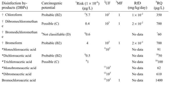
The US EPA (2003) has classified various chemicals based on their carcinogenicity potential and other detrimental effects. Generally the environmental databases report either the slope factors (SF) or concentrations corresponding to unit risk for different routes of exposures for carcinogenic compounds. Toxicity data are obtained through laboratory experiments and epidemiological studies. Either extrapolation models or uncertainty (and modifying) factors are used to convert animal toxicity data like no-observed- allowable-effect-concentration (NOAEL) and low-observed-allowable-effect-concentration (LOAEL) to estimate reference dose (RfD) for non-cancer risk effects. The threshold concentration for non-cancer risk effects can be

determined from risk quotient (RQ = 1), which is the ratio of exposure concentration (converted into dose based on exposure time) to RfD. In this paper, four species of THMs and two HAAs are selected for the fuzzy synthetic evaluation of drinking water in distribution system (see Table 3).

The three-step process, of fuzzification, aggregation and defuzzification is commonly used for fuzzy-based decision-making (Lu et al., 1999). This approach is employed here to translate observations to risk levels, and is referred to as fuzzy synthetic evaluation (FSE).

2.1. MEMBERSHIP FUNCTIONS FOR CANCER AND NON-CANCER RISKS - FUZZIFICATION

DBPs have potential to cause human cancer and non-cancer risks through consumption of drinking water. The four species of THMs - TCM, DBCM, BDCM and TBM - and two

haloacetic acids – DCAA and TCAA – are used in this analysis. For both cancer and non-cancer risks the triangular fuzzy numbers (TFNs) are defined using three partitions – low, medium and

high risk as shown in Table 4. For cancer effects, the low risk is defined as less than one in a million (10-6) and the high risk is defined as more than one in ten thousands (10-4). The

intermediate range is defined as medium risk. To fuzzify this information the TFN for low risk is defined such that the membership µ of 0.0 is assigned at the midpoint of the medium risk.

Similarly, for high risk TFN the µ of 0.0 is assigned at the midpoint of the medium risk. The membership of medium risk over the universe of discourse is defined as

H L

M µ µ

µ =1− − (1)

For non-cancer effects, the low risk is defined for concentration at risk quotient RQ ≤ 0.01 and high risk is defined for concentration of RQ > 1. The intermediate range is defined as

medium risk. To fuzzify this information, the TFN for low risk is defined such that the

membership µ of 0.0 is assigned at the midpoint of the medium risk (concentration corresponding to RQ of 0.1). Similarly, for high risk TFN, the µ of 0.0 is assigned at the midpoint of the

medium risk. The membership for medium risk over the universe of discourse is estimated using

equation 1 (see Table 4).

2.2. WEIGHTING SCHEME

Fuzzy synthetic evaluation requires information for relative importance of attributes or criteria (e.g., for various DBPs species). The relative importance is established by a set of

preference weights, which can be normalized to a sum of 1. In case of n criteria, a set of weights can be written as ) w ,..., w , w ( W = _{1 2 n} where ∑ = (2) = n j j w 1 1

Saaty (1988) proposed an analytical hierarchy process (AHP) to estimate the relative importance of each attribute (in a group) using pair-wise comparisons. Lu et al. (1999), Sadiq et

al. (2004b), and Khan et al. (2002) also used a similar technique for calculating the weights of

multiple attributes. The relative importance of different factors is assigned using intensity of importance using factors from 1 to 9, where 1 represents “equal importance” and 9 represents “extreme importance” (see Saaty (1988) for detail). An importance matrix, J, can be established, where each element, jmn, in the upper triangular matrix expresses the importance intensity of a criterion (or property) m with respect to another criterion n. For example, in the importance matrix, J, below, chloroform has been assigned importance intensities 2 and 3 times greater than DBCM and BDCM, respectively for cancer effects. Each element in the lower triangle of the matrix is just the reciprocal of an element in the upper triangle, i.e., jnm = 1/jmn. The importance matrix J, for cancer risk was thus developed as an example:

TCM DBCM BDCM TBM DCAA TCAA TCM _{1 2 3 1 1 2} DBCM _{0.5 1 1.5 0.5 0.5 1} J = BDCM 0.33 0.67 1 0.33 0.33 0.67 TBM 1 2 3 1 1 2 DCAA _{1 2 3 1 1 2} TCAA _{0.5 1 1.5 0.5 0.5 1} (3)

The importance value of each element, jmn, in J matrix above should be assigned based on expert opinion on how the different DBPs species affect human health under the specific circumstances. In thiscase, the US EPA (2003) carcinogenicity potential ranking system is used to assign importance factors (see Table 3). Members jmn can be modified as required if better information becomes available. A matrix I can be determined by taking the geometric mean of each row and then the weighted vector W can be derived by normalization of matrix I.

                    =                     = ⇒                     = 115 0 231 0 231 0 077 0 115 0 231 0 76 0 51 1 51 1 50 0 76 0 51 1 . . . . . . w w w w w w W . . . . . . I TCAA DCAA TBM BDCM DBCM TCM cancer (4)

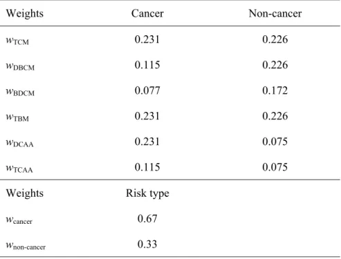
The weighted vector Wcancer indicates that TCM, TBM and DCAA will contribute more to overall cancer risk because of their higher carcinogenicity potential (defined as B2 in US EPA ranking system). Similarly, the importance matrix (J) is established for non-cancer risk and the weights for non-cancer risk are estimated. The weights estimated (for DBPs) causing cancer and non-cancer risks are summarized in Table 5. In the second stage, the final weights for cancer and cancer risks are estimated by assigning cancer risk 2 times more importance than the non-cancer risks (Lee, 1992). The aggregation process is shown in Figure 1.

2.3. AGGREGATION

Table 4 is used to establish the membership for TFNs of cancer and non-cancer risks caused by consumption of drinking water. As described before, risk in each case is defined by three partitions - low (L), medium (M), and high (H). The memberships of these partitions (risk levels) are used to establish an evaluation matrix A, where each row represents levels of cancer (or non-cancer) risk due to various DBPs. The weight vector

is multiplied (cross product) by matrix A to determine matrix B

[

]

[

]

[

]

Similarly for non-cancer risk the matrix Bnon-cancer will be

[

]

The final fuzzy evaluation matrix for risk R can be determined as

[

]

[

]

The contribution of each DBP in the aggregation process provides only a “partial evidence” to the intensity of final risk. Though the memberships of DBPs to low, medium and

high risks are monotonic over the universe of discourse, but it does not guarantee that the final

fuzzy set for risk will maintain that sequence, especially in the extreme cases where some parameters have “high value” memberships to low risk, and others have “high value” memberships to high risk. To make this process more meaningful and intuitive, defuzzification is

performed. It can be achieved through maximising risk membership in matrix R (Cheng and Lin, 2002).

(

)

K represents the predominant risk level i.e. the highest value of membership, which

decides the overall risk classification. The crisp value of risk can also be determined by assigning weights to memberships of the risk matrix (Lu et al., 1999; Silvert 2000). For example, the following equation is used for defuzzification in this study:

H M L r . r r . RI index Risk = =05× +1× +23× (8)

The coefficients (weights) are assigned arbitrarily in this study and guidelines may be established for risk-index (Lu et al., 1999). To make the risk-index more meaningful, the coefficients are adjusted so that the risk-index matches the threshold suggested by regulatory agencies. The US EPA (2001) has suggested maximum contaminant levels for total THMs (80 µg/L) and HAAs (60 µg/L). The water will be declared unfit for drinking if any of the ratios will exceed 1.0. The water will be considered safe for drinking if the following equation holds:

0 1 60 80 . HAAs of ion Concentrat , THMs of ion Concentrat max Method . Std _≤            ∑       ∑ = (9)

For example if the standard method (equation 9) ratio is estimated at 0.5, it implies that the concentration of either THMs or HAAs (which ever is the highest) is half of the threshold (guideline value). The maximum operator is used because of its conservativeness. Though if the ratio exceeds 1 (regardless of how big is the ratio), implication is that the regulatory thresholds are violated.

To make proposed index more meaningful, the risk-index estimated by fuzzy synthetic evaluation technique can be linked to standard method ratio using simpleregression analysis:

) RI ( f Method . Std = (10)

3. APPLICATION

The fuzzy synthetic evaluation procedure described in section 3 was applied to two case studies in the Quebec City region (Canada). The application relies on data on chlorinated DBPs generated under experimental chlorination of waters of two utilities: Quebec City and Sainte-Foy. The data represent the potential occurrence of DBPs in the distribution systems of the utilities. The Quebec City utility takes the water from a river with high colour content while Sainte-Foy utility takes the water from the Saint-Lawrence River, which is low in colour but contains relatively high turbidity. The water treatment process is similar for both utilities (pre-oxidation, coagulation, sedimentation, filtration, disinfection with ozone, and post-disinfection with chlorine). The main difference between the water treatment procedures of the two utilities is that Quebec City uses pre-chlorination of raw water while Sainte-Foy uses pre-ozonation.

3.1. DATA COLLECTION

For each utility, eighteen samples of post-ozonated water were chlorinated from Feb. 2001 to Jan. 2002. Once each sample was collected, it was then subjected to bench-chlorination with 2.5 mg/L dose (using sodium hypo-chlorite). This represents the maximum

post-chlorination dose applied in both utilities. The water temperature measured in the field was reproduced in the laboratory and the pH was set to 7.5 (the average value found in distribution systems for both utilities). Once chlorine was applied, THMs and HAAs were measured following six different contact times varying from 15 min to 1, 2, 6, 24 and finally to 48 hours. These contact times represent theoretical residence times of water in the distribution systems of both utilities.

THMs and HAAs were analysed according to US EPA methods 551.1 and 552.2, respectively (USEPA, 1990; USEPA, 1995). Samples for THMs and HAAs analysis were extracted using pentane and methyl-tert-butyl-ether, respectively. After sample extraction, analysis for THMs and HAAs was conducted by means of two Perkin Elmer auto-system XL gas chromatographs with electron capture detectors (Rodriguez and Sérodes, 2001; Sérodes et al., 2003). For THM species, analytical protocols ensured detection limits of 0.5 µg/L for TCM and of 0.3 µg/L for BDCM, DBCM, and TBM. Detection limits for DCAA and TCAA were 1.1 and

0.6, respectively. The concentrations of other HAAs were always below the detection limits, so they were not included in this analysis.

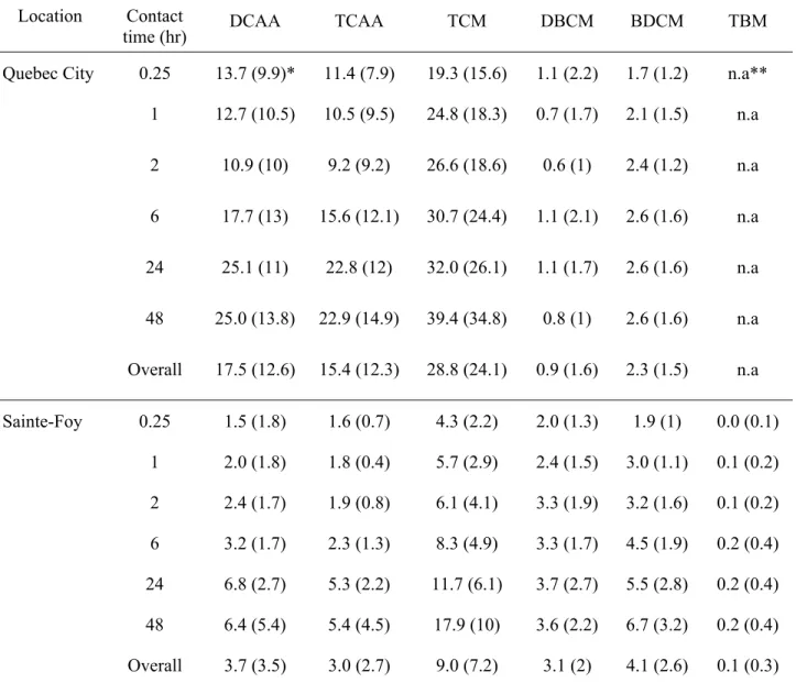
Table 6 presents the statistical portrait of the chlorinated DBPs identified according to the experimental protocol. If the values were found below detection limits, half of the detection limit values was assumed in the analysis for selected compounds. As observed, mostly

non-brominated DBPs were identified in the waters of the utilities under study. This may be

explained with the help of low bromide levels in the source water (<10 µg/L), which is typical of most Canadian inland waters (Health Canada, 1995). In the waters of both utilities,

concentrations of THMs and HAAs increased with contact time. However, the levels of most species stabilized after 24 hours of contact.

Increasing contact times assure more DBPs concentrations in the water distribution systems. The data are reported with respect to season and chlorine contact time. The contact time is used as a surrogate for water residence time in the distribution system, which shows spatial variability in DBP concentration.

3.2. FUZZY ANALYSIS

The application of the fuzzy synthetic evaluation procedure allowed estimation of the potential risks related to DBPs in waters from the two utilities. Both DBP cancer and non-cancer risks were evaluated. Figures 2 and 3 represents seasonal variations of risk memberships (low,

medium and high) for Quebec City and Sainte-Foy, respectively. Figure 2 represents risk

memberships for 0.25, 2, 6 and 24 hour contact times for Quebec City water samples. It can be noticed that membership in low risk decreases as the contact time increases. But at the same time the memberships to medium and high risk increase. Seasonal effects are also very prominent; as the temperature increases (summer season), the memberships in low risk decreases and in

medium and high risk increases. Such seasonal effects appear more significant for high contact

times. Results concerning seasonal and contact time variations are similar for the Sainte-Foy water (see Figure 3). However, the memberships in low risk and high risk for Sainte-Foy are much higher and much lower, respectively, than Quebec water (see Table 7). These results suggest that, although the average concentrations of THMs and HAAs are lower than regulated levels (Table 2), the potential risk that related to these DBPs is higher in Quebec City than in

Sainte-Foy water. This result can be explained by the strategies used by these two utilities for raw water pre-oxidation. Thus, the use of pre-ozonation in Sainte-Foy would reduce significantly the potential of cancer and non-cancer risks related to chlorinated-DBPs in the distribution system.

The risk memberships were subsequently used to evaluate the risk indices using equation 8. The US EPA levels for total THMs (80 µg/L) and HAAs (60 µg/L) were then used to estimate the ratio of DBPs concentrations with respect to their threshold levels and the maximum value of the ratio (standard method value) was taken as a representative estimate. The risk indices for Quebec City data were then compared with standard method ratios to develop a predictive model. A simple linear regression model was developed, and the equation is given below. The model has an R2 value of 0.76 (Figure 4).

( )

The above model was used to predict the standard method ratios for Sainte-Foy. Figure 5 shows the estimated ratios for the standard method (based on data collected) and the ratios predicted using the above model. A high value of R2 (0.82) was observed for the data, which indicates the good predictive capability of this model.

3.3. SENSITIVITY ANALYSIS

Sensitivity analysis is the process of estimating the degree to which outputs of a model change as the values of input parameters are changed. As mentioned before that the standard method (given in equation 9) ratio exceeding “1” means violation of regulated guidelines. Figure 6 shows the sensitivity analysis results with respect to variability in TCM concentrations. The concentrations for other five species are fixed at 10 µg/L in this example. As the concentration of TCM approaches to 50 µg/L (remaining 3 THM species have total concentration of 30 µg/L), the standard method ratio becomes steady at 1.0, but a gradual changes in memberships of low,

medium and high risks, and risk index (RI) can be noted. Another important point is that though

the total concentration of two HAAs species is 20 µg/L, but it does not play any role in standard ratio method, whereas the proposed method fully takes their contribution towards final risk memberships. Similar type of sensitivity analysis can be performed for other DBPs.

4. DISCUSSION

In aggregation or grouping process, recognition of two potential pitfalls namely

exaggeration and eclipsing is important. Exaggeration occurs when all basic items are of

relatively low risk, yet the final risk comes out unacceptably high. Eclipsing is the opposite phenomenon, where one or more of the risk items is of relatively high risk, yet the estimated aggregative risk comes out as unacceptably low. These phenomena are typically affected by the aggregation method used, thus the challenge is to determine the best aggregation method which will simultaneously reduce both exaggeration and eclipsing (Ott, 1978).

Aggregation operators used for the development of environmental indices generally include additive forms (simple addition, arithmetic average, weighted average), root sum power, root sum square, maximum, multiplicative forms (e.g., geometric mean, weighted product), and minimum operators (Silvert, 2000; Somlikova and Wachowiak, 2001; Ott, 1978).

The proposed approach has several advantages:

• It enables the synthesis of both cancer and non-cancer risk data into a single framework; • It assigns memberships to various levels of risk instead of a crisp number (like threshold

value of guidelines) and propagates that vagueness throughout the grouping process; • Its modular form is scalable; enabling the accommodation of new knowledge and

information, such as more species of DBPs and other water quality indicators;

• It can be used to guide decision-making to focus attention on those areas which have the most adverse impact on final risk;

• More toxicity data will increase the reliability of this method and can also help pinpoint those areas in which more data would yield the highest benefits; and

• It is easily programmable for computer applications and can become a risk analysis tool for a water distribution system;

• It may be sensitive for the selection of weights and aggregation operators. A trial and error approach may be required to avoid exaggeration and eclipsing;

• No interaction effects (synergistic or antagonistic) are considered while developing risk indices and various species of DBPs are assumed to have independent effects; and

• This framework accommodates both highly reliable and less reliable data. Some toxicity data may be supported by rigorous observations, while other data may be based on extrapolation models. These two types of data should have different weights in the aggregation process. The structure in its current form does not address this need to distinguish between data obtained from sources of different reliabilities.

The structure presented in this paper is a simplified demonstration of the approach. A comprehensive structure would require a major effort, including the collaboration of several experts in the various disciplines of water quality.

5. SUMMARY AND CONCLUSIONS

The water in distribution networks may contain various types of DBPs, which are harmful for human health. The quantification and characterization of risk in water distribution systems is a complex process. In this study, a risk-index was developed using cancer and non-cancer risk data of THMs and HAAs. A fuzzy synthetic evaluation technique is applied for aggregating risk posed by various DBPs species. An analytic hierarchy process was used for the aggregation of the risk items. Weighted average operators were used for grouping various risk items that may be expressed in non-commensurate units. The selection of appropriate aggregation operators can be challenging. Future research should develop a comprehensive system, including expert panels, and processes for the selection of the most appropriate aggregation operators.

Future research must also consider other chlorinated-DBPs (e.g., acetonitriles) and non-chlorinated DBPs occurring in drinking water such as those produced by disinfection with ozone (i.e., bromates) and with chlorine dioxide (i.e., chlorite and chlorate). Indeed, several water utilities (even those presented in this study) use more than one type of disinfectant. Thus, an improved risk-index must integrate the risk related to non-chlorinated DBPs. In addition, future

work must also be carried out to establish a unified risk-index by incorporating potential infectious risk associated with microbiological water quality.

In the model development stages, the risk-index is expected to have limited meaning for the acceptability of risk by public. It is envisaged that as this model is developed, populated and subsequently improved upon (using newly obtained data) the developers will gain insight into acceptable risk levels as they are manifest in the final fuzzy and/or defuzzified risk values. In the longer term, this approach could serve as a basis for bench marking acceptable risk due to DBPs in water distribution system.

As shown that a good correlation exists between standard method and the proposed risk index, it can be concluded that what can be achieved through former, can be predicted by proposed approach (meaning whether meeting regulatory requirements or not). In addition, the proposed approach also provides the memberships to various risk levels, which can not be inferred from standard US EPA method. The evaluation of risk, based on the fuzzy-synthetic evaluation procedure presented in this paper, can be applied by different users: water managers (for example for selecting between water treatment procedures according to the DBP risk reduction), government managers responsible for regulations (e.g., as a decision-making tool to regulate specific DBPs) and environmental epidemiologists (e.g., to estimate human exposure to DBPs in drinking water for cancer and non-cancer epidemiological studies).

The application presented here used fuzzy synthetic evaluation for risk indexing of chlorinated DBPs which were generated by laboratory-scale studies (that is, potential DBP occurrence). Once available, the method must be also validated in the future with robust full-scale data representing seasonal and spatial variations of DBPs in distribution systems.

6. REFERENCES

Aus-NZ 2000. Australian drinking water guidelines, Australian National Health and Medical Research Council, http://www.health.gov.au/nhmrc/publications/synopses/eh19syn.htm. Bonissone, P.P. 1997. Soft computing: the convergence of emerging reasoning technologies, Soft

Computing, 1: 6-18.

Cantor, K.P., Lynch, C.F., Hildesheim, M.E., Dosemeci, M., Lubin, J., Alavanja, M., and Craun, G. 1998. Drinking water source and chlorination by-products I. risk of bladder control,

Epidemiology 9(1): 21-28.

Cheng, C-H, and Lin, Y. 2002. Evaluating the best main battle tank using fuzzy decision theory with linguistic criteria evaluation, European Journal of Operation Research, 142: 174-186. Graves, C.G., Matanoski, G.M., and Tardiff, R.G. 2002. Weight of evidence for an association between adverse reproductive and developmental effects and exposures to disinfection by-products: a critical review, Regulatory Toxicology and Pharmacology; 34: 103-124. Health Canada 1995, A National survey of chlorinated disinfection by-products in Canadian

Drinking water, Government of Canada, Ottawa, 85 p.

Health Canada 2001. Summary of guidelines for drinking water quality, Federal-Provincial subcommittee, www.hc-sc.gc.ca/ehd/bch/water_quality.htm.

Khan, F.I., Sadiq, R., and Husain, T. 2002. GreenPro-I: A risk-based life cycle assessment and decision-making methodology for process plant design, Environmental Modeling and

Software, 17: 669-692.

Klir, G.J., and Yuan, B. 1995. Fuzzy sets and fuzzy logic - theory and applications, Prentice- Hall, Inc., Englewood Cliffs, NJ, USA.

Lascio, L.D., Gisolfi, A., Albunia, A., Galardi, G., and Moschi, F. 2002. A fuzzy-based

methodology for the analysis of diabetic neuropathy, Fuzzy Sets and Systems, 129: 203-228. Lawry, J. 2001. A methodology for computing with words, International Journal of Approximate

Reasoning, 28: 51-89.

Lee, H.-M. 1996. Applying fuzzy set theory to evaluate the rate of aggregative risk in software development, Fuzzy Sets and Systems, 79: 323-336.

Lee, Y.W. 1992. Risk assessment and risk management for nitrate contaminated groundwater

supplies, PhD dissertation, Department of Civil Engineering, University of Nebraska,

Linder, R.E., Klinefelter, G.R., Strader, L.F., Suarez, J.D., and Dyer, C.J. 1994. Acute

spermotogenic effects of bromoacetic acid, Fundamentals of Applied Toxicology, 22: 422-430.

Lu, R.-S., and Lo, S-L. 2002. Diagnosing reservoir water quality using self-organizing maps and fuzzy theory, Water Research, 36: 2265-2274.

Lu, R-S., Lo, S-L, and Hu, J-Y. 1999. Analysis of reservoir water quality using fuzzy synthetic evaluation, Stochastic Environmental Research and Risk Assessment, 13: 327-336.

Maier, S.H. 1999. Modeling water quality for water distribution systems, Ph.D. thesis, Brunel University, Uxbridge.

NTP 1998. Bromochloroacetic acid: Short term reproductive and developmental toxicity study

when administered to Sprague-Dawley rats in the drinking water, NTP-RDGT NO. 96-001,

National Toxicology Program, Maryland

Ott, W.R. 1978. Environmental indices: theory and practice, Ann Arbor Science Publishers Inc., pp. 371.

Rodriguez, M.J. and Sérodes, J.B. 2001. Spatial and temporal evolution of trihalomethanes in three water distribution systems, Water Research, 35:1572-1586.

Saaty, T.L. 1988. Multicriteria decision-making: the analytic hierarchy process, University of Pittsburgh, Pittsburgh, Pa, USA.

Sadiq, R., Kleiner, Y., and Rajani, B.B. 2004a. Aggregative risk analysis for water quality failure in distribution networks, Aqua -Journal of Water Supply: Research and Technology (In press).

Sadiq, R., Kleiner, Y., and Rajani, B.B. 2003. Water quality failure in distribution networks: a framework for an aggregative risk analysis, AWWA Annual Conference, June 2003, Anaheim, California.

Sadiq, R., Rajani, B.B., and Kleiner, Y. 2004b. A fuzzy-based method to evaluate soil corrosivity for prediction of water main deterioration, ASCE Journal of Infrastructure Systems (In press). Serodes, J-B, Rodriguez, M.J., Li, H. and Bouchard, C. 2003. Occurrence of THMs and HAAs in

experimental chlorinated waters of the Quebec City area (Canada), Chemosphere, 51: 253-263.

Sharfenaker M.A. 2001. US EPA offers first glimpse of stage 2 D/DBPR, Journal of American

Water Works Association, 93(12): 20-34.

Silvert, W. 2000. Fuzzy indices of environmental conditions, Ecological Modelling, 130(1-3): 111-119.

Sinha, R., Gupta, P., and Jain, P.K. 1994. Water quality modeling of a city water distribution system, Indian Journal of Environmental Health, 36(4): 258-262.

Somlikova, R., and Wachowiak, M.P. 2001. Aggregation operators for selection problems, Fuzzy

Sets and Systems, 131: 23-34.

Swamee, P.K., and Tyagi, A. 2000. Describing water quality with aggregate index, Journal of

Environmental Engineering, ASCE, 126(5): 451-455.

United Kingdom 2000. Water supply regulations for England and Wales,

www.dwi.detr.gov.uk/regs/si3184/3184.htm.

US EPA 1990. Determination of chlorination disinfection by-products and chlorinated solvents

in drinking water by liquid-liquid extraction and gas chromatography with electron-capture detection, Environmental monitoring systems laboratory office of research and development,

Method 551.1, United States Environmental Protection Agency, Cincinnati, Ohio.

US EPA 1995. Determination of haloacetic acids in drinking water by liquid-liquid extraction

and gas chromatography with electron-capture detection, National exposure research

laboratory office of research and development, Method 552.2, United States Environmental Protection Agency, Cincinnati, Ohio.

US EPA 1999. Microbial and disinfection by-product rules – simultaneous compliance guidance

manual, United States Environmental Protection Agency, EPA 815-R-99-015.

US EPA 2001. National primary drinking water standards, United States Environmental Protection Agency, EPA 816-F-01-007.

US EPA 2003. Integrated risk information system (IRIS), United States Environmental Protection Agency Database, Washington DC.

WHO 1993. Guidelines for drinking-water quality, 2nd Edition, Volume 1, Recommendations, World Health Organization, Geneva.

Yager, R.R. 1980. A general class of fuzzy connectives, Fuzzy Sets and Systems, 4: 235-242. Zadeh, L.A. 1996. Fuzzy logic computing with words, IEEE Transactions – Fuzzy Systems, 4(2):

Table 1. Toxicological information on DBPs (modified after US EPA, 1999)

DBPs Compound Detrimental effects

Chloroform Cancer, liver, kidney, and reproductive effects

Dibromochloromethane Nervous system, liver, kidney, and reproductive effects Bromodichloromethane Cancer, liver, kidney, and reproductive effects

Trihalomethanes (THMs)

Bromoform Cancer, nervous system, liver and kidney effects Dichloroacetic acid Cancer, reproductive and developmental effects Haloacetic acids

(HAAs)

Table 2. DBPs (in µg/L) regulations in various jurisdictions of the world

Compound Acronym WHO

(1993) US EPA (2001) Canada (2001) Aus-NZ (2000) UK (2000) Trichloromethane (chloroform) TCM 200 0 2 Dibromochloromethane DBCM 100 02 Bromodichloromethane BDCM 60 602 Tribromomethane (bromoform) TBM 100 0 2 Total trihalomethanes TTHM 1 WHO THM 4 1 i ∑ ≤ = 80 100 250 100

Monochloroacetic acid MCAA 150

Dichloroacetic acid DCAA 50 100

Trichloroacetic acid TCAA 100 100

Haloacetic acids HAA5 60 1

1: Under consideration

Table 3. Carcinogenic and non-cancer risk information for selected DBPs Disinfection by-products (DBPs) Carcinogenic potential 1_{Risk (1 × 10}-6₎ (µg/L) 2_UF 3_{MF RfD} (mg/kg/day) 4_RQ (µg/L) † Chloroform Probable (B2) 55.7 103 1 1 × 10-2 350 † Dibromochloromethan e Possible (C) 0.4 10 3 1 2 × 10-2 700 † Bromodichloromethan e 6

Not classifiable (D) 80.6 No data 760

† Bromoform Probable (B2) 4 103 1 2 × 10-2 700

*Monochloroacetic acid 9105 No data 91

*Dichloroacetic acid Probable (B2) 80.5 No data 1050

*Trichloroacetic acid Possible (C) 81 No data 10100

*Monobromoacetic acid 11105 No data 62

*Dibromoacetic acid 12105 No data 610

Bromochloroacetic acid 13103 1 No data 1400

1: Concentration corresponding to unit risk of 1 in a million

2: Uncertainty factor; 3: Modifying factors - these are factors used to convert NOAEL and LOAEL into RfD 4: Concentration estimated at risk quotient (RQ) = 1;

where RQ = Dosage/RfD and Dosage = [Concentration × intake rate/body weight] 5: Estimated from slope factor (SF) of 0.0061 (mg/kg/day)-1; where Risk = Dosage × SF 6: Also classified as B2 (see IRIS, US EPA, 2003)

7: US EPA (2001) and WHO (1993) 8: Derived from RQ/100

9: LD50 = 260 mg/kg/day (Berardi et al., 1987), the UF = 105 is assumed to estimate conc. corresponding to RQ = 1

10: WHO (1993)

11: LD50 = 177 mg/kg/day (Linder et al., 1994), the UF = 10 5

is assumed to estimate conc. corresponding to RQ = 1 12: LD50 = 1737 mg/kg/day (Linder et al., 1994), the UF = 105 is assumed to estimate conc. corresponding to RQ = 1

13: NOAEL = 41 mg/kg/day (NTP, 1998), the UF = 103 is assumed to estimate conc. corresponding to RQ = 1 † : Included in THMs (a group of 4 trihalomethanes, the US EPA (2001) recommended the value of 80 µg/L) *: Included in HAA5 (a group of 5 haloacetic acids, the US EPA (2001) recommended the value of 60 µg/L)

Table 4. Triangular fuzzy numbers for cancer and non-cancer risks Compounds 1µL 2µM 3µH Cancer TCM [<5.7, 5.7, 57] [5.7, 57, 570] [57, 570, >570] DBCM [<0.4, 0.4, 4] [0.4, 4, 40] [4, 40, >40] BDCM [<0.6, 0.6, 6] [0.6, 6, 60] [6, 60, >60] TBM [<4, 4, 40] [4, 40, 400] [40, 400, >400] DCAA [<0.5, 0.5, 5] [0.5, 5, 50] [5, 50, >50] TCAA [<1, 1, 10] [1, 10, 100] [10, 100, >100] Non-cancer TCM [<3.5, 3.5, 35] [3.5, 35, 350] [35, 350, >350] DBCM [<7, 7, 70] [7, 70, 700] [70, 700, >700] BDCM [<0.6, 0.6, 6] [0.6, 6, 60] [6, 60, >60] TBM [<7, 7, 70] [7, 70, 700] [70, 700, >700] DCAA [<0.5, 0.5, 5] [0.5, 5, 50] [5, 50, >50] TCAA [<1, 1, 10] [1, 10, 100] [10, 100, >100] Concentration (µg/L) µ = 1 µ = 0 1

[value with respect to membership 1, value with respect to membership 1, value with respect to membership 0]

2

[value with respect to membership 0, value with respect to membership 1, value with respect to membership 0]

3

Table 5. Weights estimated by AHP for grouping of DBPs

Weights Cancer Non-cancer

wTCM 0.231 0.226 wDBCM 0.115 0.226 wBDCM 0.077 0.172 wTBM 0.231 0.226 wDCAA 0.231 0.075 wTCAA 0.115 0.075

Weights Risk type

wcancer 0.67

Table 6. Statistical portrait (average and standard deviation of concentration are shown, µg/L) for DBPs species for waters of the two utilities for around the year sampling

Location Contact

time (hr) DCAA TCAA TCM DBCM BDCM TBM

Quebec City 0.25 13.7 (9.9)* 11.4 (7.9) 19.3 (15.6) 1.1 (2.2) 1.7 (1.2) n.a** 1 12.7 (10.5) 10.5 (9.5) 24.8 (18.3) 0.7 (1.7) 2.1 (1.5) n.a 2 10.9 (10) 9.2 (9.2) 26.6 (18.6) 0.6 (1) 2.4 (1.2) n.a 6 17.7 (13) 15.6 (12.1) 30.7 (24.4) 1.1 (2.1) 2.6 (1.6) n.a 24 25.1 (11) 22.8 (12) 32.0 (26.1) 1.1 (1.7) 2.6 (1.6) n.a 48 25.0 (13.8) 22.9 (14.9) 39.4 (34.8) 0.8 (1) 2.6 (1.6) n.a Overall 17.5 (12.6) 15.4 (12.3) 28.8 (24.1) 0.9 (1.6) 2.3 (1.5) n.a Sainte-Foy 0.25 1.5 (1.8) 1.6 (0.7) 4.3 (2.2) 2.0 (1.3) 1.9 (1) 0.0 (0.1) 1 2.0 (1.8) 1.8 (0.4) 5.7 (2.9) 2.4 (1.5) 3.0 (1.1) 0.1 (0.2) 2 2.4 (1.7) 1.9 (0.8) 6.1 (4.1) 3.3 (1.9) 3.2 (1.6) 0.1 (0.2) 6 3.2 (1.7) 2.3 (1.3) 8.3 (4.9) 3.3 (1.7) 4.5 (1.9) 0.2 (0.4) 24 6.8 (2.7) 5.3 (2.2) 11.7 (6.1) 3.7 (2.7) 5.5 (2.8) 0.2 (0.4) 48 6.4 (5.4) 5.4 (4.5) 17.9 (10) 3.6 (2.2) 6.7 (3.2) 0.2 (0.4) Overall 3.7 (3.5) 3.0 (2.7) 9.0 (7.2) 3.1 (2) 4.1 (2.6) 0.1 (0.3) * Values in the parenthesis show standard deviation of 18 samples collected over a year for each contact time in the waters of the

two utilities

Table 7. Statistics of risk memberships for Quebec City and Sainte-Foy waters

Location Memberships Mean Stdev.

Quebec City L r 0.58 0.18 M r 0.34 0.15 H r 0.08 0.07 Sainte-Foy L r 0.73 0.15 M r 0.26 0.14 H r 0.01 0.01

Risk-index (RI) Non-cancer risk TCAA DCAA TBM DBCM BDCM TCM Cancer risk TCAA DCAA TBM DBCM BDCM TCM

rL rM rH 0.00 0.20 0.40 0.60 0.80 1.00

Feb-01 Apr-01 Jul-01 Sep-01 Nov-01 Feb-02

Date M e mb ersh ip

2a. Quebec City (0.25 hr)

0.00 0.20 0.40 0.60 0.80 1.00

Feb-01 Apr-01 Jul-01 Sep-01 Nov-01 Feb-02

Date M e mb ersh ip 2b. Quebec City (2 hr) 0.00 0.20 0.40 0.60 0.80 1.00

Feb-01 Apr-01 Jul-01 Sep-01 Nov-01 Feb-02

Date M e mb ersh ip 2c. Quebec City (6 hr) 0.00 0.20 0.40 0.60 0.80 1.00

Feb-01 Apr-01 Jul-01 Sep-01 Nov-01 Feb-02

Date M e mb ersh ip 2d. Quebec City (24 hr)

rL rM rH 0.00 0.20 0.40 0.60 0.80 1.00

Feb-01 Apr-01 Jul-01 Sep-01 Nov-01 Feb-02

Date M e mb ersh ip 3a. Sainte-Foy (0.25 hr) 0.00 0.20 0.40 0.60 0.80 1.00

Feb-01 Apr-01 Jul-01 Sep-01 Nov-01 Feb-02

Date M e mb ersh ip 3b. Sainte-Foy (2 hr) 0.00 0.20 0.40 0.60 0.80 1.00

Feb-01 Apr-01 Jul-01 Sep-01 Nov-01 Feb-02

Date M e mb ersh ip 3c. Sainte-Foy (6 hr) 0.00 0.20 0.40 0.60 0.80 1.00

Feb-01 Apr-01 Jul-01 Sep-01 Nov-01 Feb-02

Date M e mb ersh ip 3d. Sainte-Foy (24 hr)

Std. Method = 1.93 RI - 0.93 R2 = 0.76 0.0 0.5 1.0 1.5 2.0 0.0 0.5 1.0 1.5

Risk Index (RI)

Std. Method

2.0

Acceptable Not-acceptable

RI = 1.0

Figure 4. Comparison of risk-index with standard method based on US EPA regulations (Quebec City)

0.0 0.2 0.4 0.6 0.8 1.0 0.4 0.6 0.8 1.0

Risk Index (RI)

Std. Method

Observed

Predicted R

2 _{= 0.82}

Figure 5. Comparison of risk-index with standard method based on US EPA regulations (Sainte-Foy)

0.0 0.5 1.0 1.5 0 100 200 300 400 500 TCM (µg/L) Values RI Std. Method Medium risk Low risk High risk