HAL Id: hal-00328509
https://hal.archives-ouvertes.fr/hal-00328509
Submitted on 2 Jul 2007
HAL is a multi-disciplinary open access
archive for the deposit and dissemination of
sci-entific research documents, whether they are
pub-lished or not. The documents may come from
teaching and research institutions in France or
abroad, or from public or private research centers.
L’archive ouverte pluridisciplinaire HAL, est
destinée au dépôt et à la diffusion de documents
scientifiques de niveau recherche, publiés ou non,
émanant des établissements d’enseignement et de
recherche français ou étrangers, des laboratoires
publics ou privés.
regional inversions over Europe – Part 1: mapping the
atmospheric CO2 signals
C. Geels, M. Gloor, P. Ciais, P. Bousquet, P. Peylin, A. T. Vermeulen, R.
Dargaville, T. Aalto, J. Brandt, J. H. Christensen, et al.
To cite this version:
C. Geels, M. Gloor, P. Ciais, P. Bousquet, P. Peylin, et al.. Comparing atmospheric transport models
for future regional inversions over Europe – Part 1: mapping the atmospheric CO2 signals.
Atmo-spheric Chemistry and Physics, European Geosciences Union, 2007, 7 (13), pp.3479.
�10.5194/acp-7-3461-2007�. �hal-00328509�
www.atmos-chem-phys.net/7/3461/2007/ © Author(s) 2007. This work is licensed under a Creative Commons License.
Chemistry
and Physics
Comparing atmospheric transport models for future regional
inversions over Europe – Part 1: mapping the atmospheric CO
2
signals
C. Geels1, M. Gloor2, P. Ciais3, P. Bousquet3, P. Peylin3, A. T. Vermeulen4, R. Dargaville3, T. Aalto5, J. Brandt1, J. H. Christensen1, L. M. Frohn1, L. Haszpra6, U. Karstens7, C. R¨odenbeck7, M. Ramonet3, G. Carboni8, and R. Santaguida9
1National Environmental Research Institute, University of Aarhus, 4000 Roskilde, Denmark 2University of Leeds, Leeds, UK
3Laboratoire des Sciences du Climat et de l-Environnement, UMR CEA-CNRS 1572, 91191 Gif-sur-Yvette, France 4Energieonderzoek Centrum Nederland (ECN), 1755 ZG Petten, The Netherlands
5Finnish Meteorological Institute Air Quality Research, Sahaajankatu 20E 00810 Helsinki, Finland 6Hungarian Meteorological Service P.O. Box 39, 1675 Budapest, Hungary
7Max-Planck-Institut f¨ur Biogeochemie, 07701 Jena, Germany 8CESI ApA, Via r. Rubattino 54, 20134 Milano, Italy
9Italian Air Force Meteorological Service, Via delle Ville, 40, 41029 Sestola (MO), Italy
Received: 25 January 2006 – Published in Atmos. Chem. Phys. Discuss.: 11 May 2006 Revised: 8 May 2007 – Accepted: 18 June 2007 – Published: 2 July 2007
Abstract. The CO2source and sink distribution across
Eu-rope can be estimated in principle through inverse methods by combining CO2 observations and atmospheric transport
models. Uncertainties of such estimates are mainly due to in-sufficient spatiotemporal coverage of CO2observations and
biases of the models. In order to assess the biases related to the use of different models the CO2 concentration field
over Europe has been simulated with five different Eulerian atmospheric transport models as part of the EU-funded AE-ROCARB project, which has the main goal to estimate the carbon balance of Europe. In contrast to previous compar-isons, here both global coarse-resolution and regional higher-resolution models are included. Continuous CO2
observa-tions from continental, coastal and mountain sites as well as flasks sampled on aircrafts are used to evaluate the models’ ability to capture the spatiotemporal variability and distribu-tion of lower troposphere CO2across Europe.14CO2is used
in addition to evaluate separately fossil fuel signal predic-tions. The simulated concentrations show a large range of variation, with up to ∼10 ppm higher surface concentrations over Western and Central Europe in the regional models with highest (mesoscale) spatial resolution.
The simulation – data comparison reveals that generally high-resolution models are more successful than coarse mod-els in capturing the amplitude and phasing of the observed
Correspondence to: C. Geels (cag@dmu.dk)
short-term variability. At high-altitude stations the magni-tude of the differences between observations and models and in between models is less pronounced, but the timing of the diurnal cycle is not well captured by the models.
The data comparisons show also that the timing of the observed variability on hourly to daily time scales at low-altitude stations is generally well captured by all models. However, the amplitude of the variability tends to be under-estimated. While daytime values are quite well predicted, nighttime values are generally underpredicted. This is a re-flection of the different mixing regimes during day and night combined with different vertical resolution between models. In line with this finding, the agreement among models is in-creased when sampling in the afternoon hours only and when sampling the mixed portion of the PBL, which amounts to sampling at a few hundred meters above ground. The main recommendations resulting from the study for constraining land carbon sources and sinks using high-resolution concen-tration data and state-of-the art transport models through in-verse methods are given in the following: 1) Low altitude stations are presently preferable in inverse studies. If high altitude stations are used then the model level that repre-sents the specific sites should be applied, 2) at low alti-tude sites only the afternoon values of concentrations can be represented sufficiently well by current models and there-fore afternoon values are more appropriate for constraining large-scale sources and sinks in combination with transport
models, 3) even when using only afternoon values it is clear that data sampled several hundred meters above ground can be represented substantially more robustly in models than surface station records, which emphasize the use of tower data in inverse studies and finally 4) traditional large scale transport models seem not sufficient to resolve fine-scale fea-tures associated with fossil fuel emissions, as well as larger-scale features like the concentration distribution above the south-western Europe. It is therefore recommended to use higher resolution models for interpretation of continental data in future studies.
1 Introduction
Quantifying the distribution and variability of CO2fluxes
be-tween the Earth’s surface and the atmosphere is essential to understand the present state and the future behavior of carbon pools and in turn radiative forcing of the earths surface asso-ciated with atmospheric CO2. Detailed and accurate
knowl-edge of sources and sinks for atmospheric CO2down to
con-tinental and regional scales is also required to monitor and assess the effectiveness of carbon sequestration and/or emis-sion reduction policies, such as the Kyoto Protocol.
Atmospheric transport integrates over all CO2 surface
sources and sinks. Measurements of the atmospheric CO2
concentration can therefore be used in principle to quantify surface fluxes over large scales by matching them with simu-lation predictions obtained with atmospheric transport mod-els. This approach, known as inverse modelling, is still lim-ited by sparse and uneven coverage of CO2monitoring
sta-tions. The current atmospheric global observation network consisted until recently of less than 100 stations and con-tained mainly discrete biweekly flask observations from re-mote oceanic or high altitude background locations. Conse-quently, the carbon balance of the continents remains very poorly constrained in inversions and its partitioning between land regions like Europe, North America and North Asia varies among different studies depending on the included sta-tions (e.g. Fan et al., 1998; Rayner et al., 1999; Bousquet et al., 2000; R¨odenbeck et al., 2003). Furthermore, when in-version results obtained with different atmospheric transport models are compared (Gurney et al., 2002, 2003), the spread in fluxes induced by transport model differences was found to be almost as large as the uncertainties arising from the lack of adequate observations, especially over the Northern Hemisphere continents.
Recently, many new stations on continents where CO2is
measured continuously have been initiated, which can be used to constrain regional CO2 fluxes on land (Law et al.,
2002). Observation sites are chosen to be regionally rep-resentative and at the same time not too close to point-like sources like towns. Such continental-oriented network in-cludes low-altitude surface stations (eg. Haszpra, 1999), hill
and mountain sites (Aalto et al., 2002; Apadula et al., 2003; Schmidt et al., 2003), tall tower sampling of the lower part of the planetary boundary layer (Bakwin et al., 1998) and frequent aircraft profiling (Gerbig et al., 2003).
Unfortunately, the inverse modelling approach for estimat-ing carbon sources/sinks on land, based on atmospheric con-centration gradients, faces a dilemma. On the one hand, sev-eral studies indicate that continental data for constraining re-gional fluxes with sufficiently small uncertainty are needed (e.g. Gloor et al., 2000). On the other hand atmospheric CO2
records from the vegetated continents are challenging to use in inverse calculations for three reasons: 1) signals on land during summer are highly variable because of the proximity to vegetation and the large fluxes associated with photosyn-thesis and respiration, 2) the complexity of near surface air flow particularly during night is not well resolved and hard to represent with models, and 3) the mismatch in scale be-tween point-like sources associated particularly with anthro-pogenic fossil fuel emissions and model resolution. Thus, it is currently an open question how to best use continental data for source/sink estimation using transport models and inverse methods.
The resolution of atmospheric transport models tradition-ally used for inverse modeling of CO2 is on the order of
2.5◦×2.5◦ degrees longitude by latitude or coarser (like for example the models used in TransCom, see Gurney et al., 2003). Because of the heterogeneous nature of surface fluxes and transport over land this resolution is likely not sufficient to reduce uncertainties of land sources and sinks by employ-ing the new continental data. However, recent studies in-dicate that higher resolution mesoscale models are able to capture the observed variability over the continents more re-alistically (Chevillard et al., 2002b; Kjellstr¨om et al., 2002; Geels, 2003; Geels et al., 2004) than traditional coarse grid models.
While there have been extensive intercomparisons of global coarse-resolution transport models on monthly and annual time-scales, (Law et al., 1996; Bousquet et al., 1996; Gurney et al., 2003) little attention has so far been paid to quantify model differences on synoptic to diurnal scales above the continents. Partly because coarse-resolution trans-port models can only poorly resolve the short-term variabil-ity, but also because data have not been available. Currently the TransCom group has a new experiment underway to look at synoptic and diurnal variations between models (Law et al., 2005).
Here we present a coarse-to-high resolution model inter-comparison study that includes five models and recent con-tinental CO2 data from Western Europe measured during
the course of the AEROCARB project (http://www.aerocarb. cnrs-gif.fr/) as a yard stick. The purpose of this paper is to estimate the variability of the results given by a representa-tive range of different models due to the differences in the description of transport in each model. Thereby we can ob-tain a better understanding of how to use optimally the new
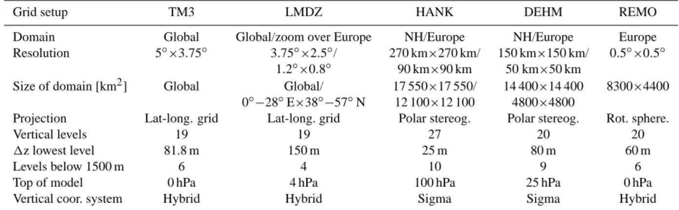
Table 1. Summary of grid set-up in the models. At European latitudes 0.5◦×0.5◦corresponds to approximately 40 km×50 km.
Grid setup TM3 LMDZ HANK DEHM REMO
Domain Global Global/zoom over Europe NH/Europe NH/Europe Europe Resolution 5◦×3.75◦ 3.75◦×2.5◦/ 270 km×270 km/ 150 km×150 km/ 0.5◦×0.5◦
1.2◦×0.8◦ 90 km×90 km 50 km×50 km
Size of domain [km2] Global Global/ 17 550×17 550/ 14 400×14 400 8300×4400 0◦−28◦E×38◦−57◦N 12 100×12 100 4800×4800
Projection Lat-long. grid Lat-long. grid Polar stereog. Polar stereog. Rot. sphere.
Vertical levels 19 19 27 20 20
1z lowest level 81.8 m 150 m 25 m 80 m 60 m
Levels below 1500 m 6 4 10 9 6
Top of model 0 hPa 4 hPa 100 hPa 25 hPa 0 hPa
Vertical coor. system Hybrid Hybrid Sigma Sigma Hybrid
Table 2. Summary of the forcing meteorology and physical parameterizations applied in the different models.
Meteorology and physics TM3 LMDZ HANK DEHM REMO Initial/boundary data NCEP ECMWF MM5/NCEP MM5/ECMWF REMO/ECMWF
1t meteorology 6 h 6 h 1 h 3 h At boundaries: 6 h,
inside: 5 min Meteorology Off-line Off-line Off-line Off-line On-line Vertical diffusion 1st order 1st order In PBL: 1st order
TKE-K-theory K-theory Holtslag and Boville (1993) K-theory 2nd order
continental CO2data in combination with models in order to
reduce the uncertainties of land sources and sinks estimates. The models used in this study span a range of resolutions, numerical schemes for solving the advection equation, pa-rameterizations of subgrid-scale processes and meteorologi-cal drivers. Identimeteorologi-cal carbon fluxes are used as surface input in all models. The input consist in yearly mean fossil fuel emissions, monthly mean air-sea exchange and hourly Net Ecosystem Exchange (NEE) fluxes with the land biosphere. By applying such a common set of surface fluxes, our model intercomparison offers the opportunity to identify the differ-ences caused by differdiffer-ences in the simulated transport and mixing processes, related to model specific parameters like the resolution. The comparison covers July and December of 1998.
The paper starts with a short description of the five tracer transport models. Next a qualitative analysis of the model differences is carried out by comparing the simulated aver-age CO2field over Europe. Thereafter the model results at
both continental and oceanic background locations are eval-uated against observed CO2records using quantitative
statis-tical evaluation criteria. Finally the main findings as well as data selection and atmospheric sampling recommendations are discussed.
In a companion paper, the same five transport models are used for simulating222Rn, which due to the comparatively time-constant nature of its source field and its short lifetime
is a useful tracer of vertical mixing and synoptic processes (Vermeulen et al., 20071). Also, regional inversions using the same models for Europe are underway (Rivier et al., 20072).
2 The set-up of the model comparison
2.1 The transport models
The five tracer transport models involved in this study cover a representative range of global and regional models used previously in various atmospheric trace gas studies. An overview of the model characteristics is given in Tables 1 and 2. In addition we briefly summarize below the main features of each model.
1Vermeulen, A. T., Ciais, P., Peylin, P., Gloor, M., Bousquet, P.,
Aalto, T., Brandt, J., Christensen, J. H., Dargaville, R., Geels, C., Heimann, M., Karstens, U., Levin, I., Ramonet, M., R¨odenbeck, C., Pieterse, G., and Schmidt, M.: Comparing atmospheric transport models for regional inversions over Europe. Mapping the 222Rn Atmospheric Signals, Atmos. Chem. Phys. Discuss., in prepara-tion, 2007.
2Rivier, L., Bousquet, P., Brandt, J., Ciais, P., Geels, C., Gloor,
M., Heimann, M., Karstens, U., Peylin, P., Rayner, P., R¨odenbeck, C., et al.: Comparing atmospheric transport models for regional in-versions over Europe. Part 2: Estimation of the regional sources and sinks of CO2using both regional and global atmospheric mod-els, Atmos. Chem. Phys. Discuss., in preparation, 2007.
TM3 is a global off-line atmospheric tracer transport model developed by Heimann (1996). Its spatial resolution is flexible and the model can be run with both coarser and finer spatial resolution than in the present study (see Table 1). TM3 is usually driven on a 6-hourly basis by re-analyzed me-teorological fields from NCEP or ECMWF weather predic-tion centers, which have to be converted and interpolated in a preprocessing step.
LMDZ (version 3.3) is a global tracer transport version of the GCM model LMDZ (Hauglustaine et al., 2004). It is a grid point global primitive equation model, which can be used for simulations with different horizontal resolutions on the global scale. The grid resolution can vary in space, which permits horizontal regional zooming (see http://www. lmd.jussieu.fr/∼lmdz/homepage.html). Here the results from LMDZ are from a global simulation with minimal resolution of 3.75◦×2.5◦ longitude by latitude including a zoom over Europe of approximately 1.2◦×0.8◦. Simulated large-scale horizontal advection is nudged to analyzed 6-hourly wind fields from ECMWF reanalyses. When compared with the models used in the Transcom 1 intercomparison experiment (Rayner and Law, 1995) (not shown), LMDZ tends to have strong large-scale horizontal as well as vertical mixing.
HANK is a nested regional transport-chemistry model re-cently developed by Hess and colleagues (2000) at NCAR. It is driven by meteorological fields simulated by the Fifth-Generation NCAR/Penn State Mesoscale Model (MM5) model system (Grell et al., 1995), which is nudged to-wards global reanalyses from National Center of Environ-mental Protection (NCEP). For additional information see http://acd.ucar.edu/models/HANK/. For the simulations per-formed for this paper a polar stereographic coordinate system with a coarse grid mesh centered at the North Pole and cov-ering approximately two thirds of the Northern Hemisphere is used. Within this larger domain, a sub-domain with three times finer resolution and centered over Europe is embedded. DEHM (Danish Eulerian Hemispheric Model) is a re-gional model that was initially developed to study long-range transport of sulphur into the Arctic (Christensen, 1997). The model has since then been further developed to include nest-ing capabilities (see Frohn et al., 2002) as well as differ-ent chemical species (Frohn, 2004; Christensen et al., 2004; Geels et al., 2004; Hansen et al., 2004). The MM5 model (Grell et al., 1995) is used as the meteorological driver for the model system, which in this setup is nudged towards reanal-yses from the European Center for Medium Range Weather Forecast (ECMWF).
REMO (REgional MOdel) is a regional climate model based on the Europamodell (EM) of the German Weather Service (DWD) (Majewski, 1991). For almost 10 years, the Europamodell has been the operational regional weather forecast model of DWD. REMO has been extended to an on-line atmosphere-chemistry model (Langmann, 2000). In the present study REMO (version 5.0) includes the physical parametrization package of DWD and is operated in a
diag-nostic mode. The results of consecutive short-range forecasts (30 h) are used. REMO is started each day at 00:00 UTC from ECMWF operational analyses and a 30-h forecast is computed. To account for a spin-up time the first six hours of the forecast are neglected. By restarting the model every day from analyses, the model state is forced to stay close to the ECMWF analyzed weather situation.
Note that the models TM3 and HANK are driven by mete-orological fields preprocessed by the National Center for En-vironmental Protection (NCEP) meteorology, while LMDZ, DEHM and REMO are driven by fields from the European Center for Medium Range Weather Forecast (ECMWF).
2.2 Prescribed surface fluxes
The net exchange of CO2used as input at the models lower
boundary in the five models, consists of fossil fuel emissions, an air-sea CO2flux, and a land photosynthesis and
respira-tion flux.
Fossil fuel CO2 emissions are obtained from the
EDGAR3.0 emission Database (Olivier et al., 1996). The data set is based on a combination of statistics on energy con-sumption, emission factors, and population density as well as information on the location of major point sources. The re-sulting global emissions have a 1◦×1◦ spatial resolution and corresponds to the year 1990. Main features for Europe are as follows: emissions are high over Central to Western Eu-rope with the highest emissions over the Benelux countries, Germany and Great Britain. Outside these regions emissions are much smaller.
Between 1990 and 1998, which is the year in focus in this study, emissions have decreased by approximately 30% over Eastern and Central Europe, but remained more or less con-stant over the Western part of Europe (Marland et al., 2003). A few studies of the14C isotopic composition of carbon indi-cates variations of fossil fuel emission on seasonal to diurnal timescales in Europe (Levin et al., 2003). The documenta-tion is, nevertheless, sparse and those variadocumenta-tions are neglected here, in absence of better resolved fossil CO2emission maps
(e.g. Blasing et al., 2005).
Air-sea flux of CO2 is prescribed according to the study
of Takahashi and colleagues (1999), who combined a cli-matological distribution of sea-air pCO2 differences and
a wind-speed dependent gas exchange coefficient (Wan-ninkhof, 1992) parameterization to estimate monthly air-sea fluxes for the global ocean with a 4◦×5◦resolution for 1995. The northernmost part of the Atlantic Ocean acts as a net sink for atmospheric CO2 throughout the year (−0.46 GtCy−1
north of 50◦N in 1995). In this study we neglect interan-nual variability of air-sea fluxes. Also there is no consistency between the wind fields used to transport CO2in the models
and those used to calculate the air-sea gas exchange. Biosphere-atmosphere exchange of CO2 (net ecosystem
exchange (NEE)) is estimated by the Terrestrial Uptake and Release of Carbon (TURC) model (Ruimy et al., 1996;
La-font et al., 2002). TURC is a light-use efficiency model driven by radiation, temperature, and humidity fields from ECMWF and 10-days composite Normalized Difference Vegetation Index (NDVI) from the SPOT4-VEGETATION sensor launched in April 1998. For January 1998 the NDVI data from 1999 have been used. The resolution of the TURC version we used is 1◦×1◦ and the calculated daily fluxes for 1998 are divided into gross primary production (GPP) and the components of Ecosystem Respiration (ER) consisting in maintenance, growth and heterotrophic respiration. In order to fully resolve the diurnal cycle, the daily fluxes have been redistributed among the 24 hours of the day using a sim-ple scaling scheme following the main characteristic of the fluxes. Growth and heterotrophic respiration are assumed to be uniform throughout the day. GPP and maintenance res-piration on the other hand are assigned a diurnal cycle fol-lowing the incoming shortwave radiation and local air tem-peratures. In the TURC model, each vegetated grid point is forced to be carbon neutral on a yearly basis (i.e. annual mean NEE=GPP−ER=0). This assumption, commonly ap-plied in studies of the seasonal variability in atmospheric CO2 (Fung et al., 1987; Denning et al., 1996) is reasonable
in our case since we focus the model evaluation on synoptic and diurnal timescales. Yet, it may bias the model-data com-parison when looking at monthly concentration gradients among sites. Note that the TURC biospheric fluxes driven by ECMWF fields are naturally more consistent with the mod-els using ECMWF winds (LMDZ, DEHM and REMO) than for the other models (TM3 and HANK).
The TURC predicted fluxes have been evaluated both by direct comparison with a few eddy covariance data in Europe (Aalto et al., 2004) and by indirect comparison against at-mospheric CO2data after being transported in atmospheric
models (Chevillard, 2001; Geels, 2003). These studies demonstrated that during summer the hourly TURC fluxes are generally reproducing quite well the observed diurnal cycle of NEE at most temperate forest eddy flux sites with regards to timing and amplitude at mid latitudes, while the diurnal NEE and hence the seasonal amplitude is underesti-mated at higher latitudes. Occasionally very high night-time respiration fluxes observed at some sites are also not properly captured by TURC.
To give an idea of the order of magnitude of the fluxes, we list here the strength of the total monthly flux for each source type within the REMO model domain (36.52×10⁶km2). In July the biosphere is a net sink of −0.35 GtC (−13.8 gC m−2
land mo−1), while a net source of 0.24 GtC (9.08 gC m−2
land mo−1) during December. The ocean acts like a net sink
of −0.05 GtC (−3.47 gC m−2 ocean mo−1) and −0.03 GtC (−2.10 gC m−2ocean mo−1) in July and December, respec-tively. Total fossil fuel emission amount to 0.17 GtC each month (6.76 gC m−2land).
The fluxes have been re-gridded from the original spatial resolution of 1◦×1◦ or 4◦×5◦ to the grid of each model. Thereby will the lower resolution models lose peak values
e.g. in the fossil fuel emissions compared to the models with a higher resolution. This means that while the net flux across Europe may be the same, there will be larger spatial vari-ability of fluxes in the higher resolution models (up to the resolution of the original surface fluxes).
2.2.1 Boundary and initial conditions
The lateral and upper boundary conditions vary from model to model. The REMO model has the smallest domain and sensitivity tests show that concentrations at its lateral bound-aries transported inside the European domain can dominate the CO2signal, especially at higher altitude stations
(Chevil-lard et al., 2002a,b). Here the global CO2 fields used at
REMO’s boundaries are prescribed at a 3h interval from sim-ulations with the global TM3 model.
Both DEHM and HANK cover the major part of the North-ern Hemisphere and we assumed that the spatiotemporal pat-tern of the simulated CO2 field within Europe during one
month is negligibly affected by the sources and sinks outside the domain. For these two models the CO2 concentration
was therefore assumed to be constant (0 ppm) at the lateral and upper boundaries.
Also the initial conditions differ among the models. The TM3, LMDZ and DEHM models were run for the full year of 1998 and include several months of spin up (from a con-centration of 0 ppm) before the July and December months that we focus on here. This is also the case for the REMO model, which is initialized with TM3 results. HANK in con-trast is started up from 0 ppm on July 1st and December 1st, respectively. Preliminary tests that we made showed that the initial conditions get rapidly mixed up homogeneously over Europe within 3–5 days. Yet the results from HANK should be interpreted during the first week of each month with this caveat in mind.
In the following, the concentration fields from the five models have been referenced to the simulated monthly av-eraged CO2at Mace Head (53.33
◦
N, 9.90◦W) both in the maps and in the time-series plots. Here the term ”referenced” means that the value at Mace Head has been subtracted in each grid cell, see Fig. 2 for a range across the models for this value. Thereby possible biases due to differences in ini-tial conditions are minimized.
3 Results: surface distributions
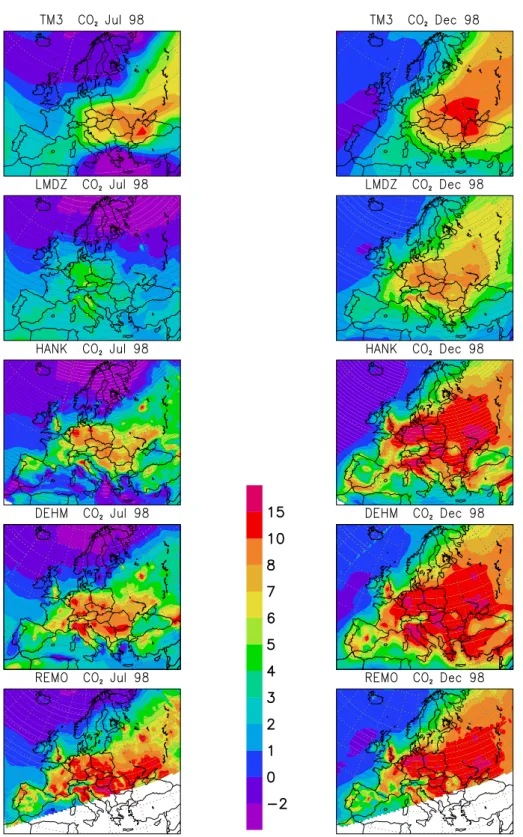
In order to investigate model differences, mean simulated CO2 distributions for July and December are displayed in
Fig. 1 for all five models. Before comparing the models with each other and later with observations it is important to rec-ognize the influence of vertical resolution, especially within the lowest few hundred meters above the ground. As seen in Table 1 the depth of the lowest model layer varies be-tween 25 m in HANK up to 150 m in LMDZ. The simulated
Fig. 1. Mean monthly CO2concentrations (in ppm) for July and December 1998, as simulated by the five transport models. Each model output has been interpolated to 11 hPa above ground and is displayed relative to the monthly CO2level at Mace Head, Ireland.
surface concentrations will hence represent mean CO2
con-centrations over different portions of the air column. In order to harmonize the intercomparison, each model output was
in-terpolated to 11 hPa above ground, which is the center of the lowermost layer of the coarsest model (LMDZ).
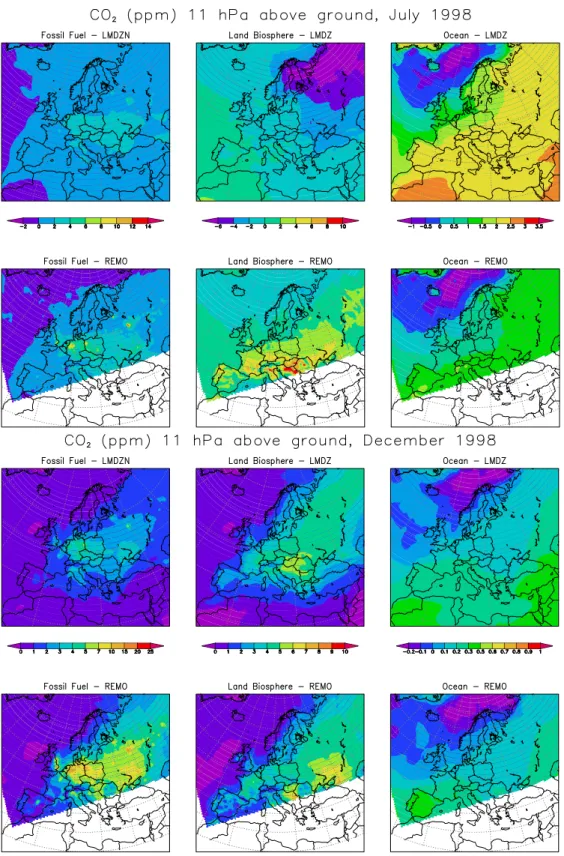
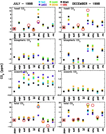
Fig. 2. The separated components for July and December, as simulated by the LMDZ and REMO models. Displayed relative to the monthly
CO2level at Mace Head, Ireland. The level at Mace Head in July for LMDZ/REMO (in ppm): 3.0/13.2 (fossil fuel), −2.9/−4.8 (biosphere),
3.1 Spatial patterns for July
The overall pattern of the July monthly mean concentra-tion field is qualitatively similar among the five models with highest CO2 values over the continent and lower values
over the Northeast Atlantic and in some of the models over the Mediterranean (Fig. 1). LMDZ seems to be an outlier with generally lower surface concentrations indicating faster boundary layer ventilation. Despite the qualitative agreement there are large quantitative differences (up to about 10 ppm). Furthermore there is a difference between coarser-resolution global model and regional model simulations: There is more fine-scale structure in the latter and there is an eastward (downstream) shift in the concentration maximum caused by fossil fuel emissions in the global models.
In order to investigate the differences between models in more detail, we show in Fig. 2 each component for July for the two most contrasting models, REMO and LMDZ.
In the simulations of fossil fuel CO2, the impact of the
het-erogeneity of the emission field is evident. The increase in horizontal resolution leads to an increase in small scale fea-tures being better resolved, such as for example positive CO2
anomalies over large cities in the regional model REMO. The simulations of the NEE component alone indicate that the interplay between NEE and convective mixing is the main reason why total CO2 differs among the models. In July,
when the vegetation is active, alteration of near ground CO2
varies inversely with mixing within the PBL, as shown for instance in tall tower records (Bakwin et al., 1998), global models (Denning et al., 1996) and in regional model studies (Chevillard et al., 2002b; Geels, 2003). As mixing during night is usually much less than during day, nighttime respira-tory CO2accumulates in a shallow nocturnal boundary layer,
while the low CO2concentrations due to photosynthesis are
diluted over a deeper convective PBL during daytime. Thus even if the daily integrated CO2exchange between land
veg-etation and atmosphere is zero there will be a positive CO2
signal at the surface. The degree to which models are able to capture this “diurnal rectification” will be discussed in more detail in Sect. 5.
The substantial difference between the global LMDZ and regional REMO simulations for the biospheric CO2
compo-nent is mainly related to vertical mixing and vertical resolu-tion of the models. This indicates that near-ground vertical resolution plays an important role in predicting near-ground concentrations, the realism of which will be discussed later on.
The oceanic component in both LMDZ and REMO low-ers the atmospheric CO2 content over the northern part of
the Atlantic by approximately 0.5–1.0 ppm relative to Mace Head. The largest dissimilarity between the two simulations is over land where the concentration gradient is steeper in the LMDZ results.
The large differences in mean signals across model sim-ulations and the recognition that a main cause is the
differ-ence in modeling nighttime concentrations suggest investi-gating alternative sampling schemes. In particular it is natu-ral to try to take advantage of convective mixing on land dur-ing days with fair weather conditions. For such conditions near ground observations are similar to PBL concentrations (Bakwin et al., 1998) and likely as well much more homoge-neous in the horizontal direction in comparison to night-time concentrations. To assess this assertion we define in the fol-lowing daytime sampling as sampling restricted to the period from 10:00–17:00 Local Standard Time (LST).
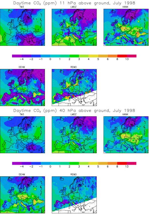
As seen in Fig. 3 the difference among models in July is less dramatic for daytime averages compared to the whole-day averages shown in Fig. 1. The differences are reduced further for daytime sampling at a few hundred meters above ground (here at 40 mbar ≃400 m), as seen in Fig. 3. In REMO, HANK and to some degree DEHM and LMDZ higher concentrations are seen over oceanic coastal regions during daytime for July at 11 hPa above ground. A possi-ble explanation could be the land sea-breeze combined with the surface exchange and atmospheric mixing. Near-ground night-time air enriched in respired CO2is transported from
land to the adjacent sea during night. Over land the night-time air enriched with CO2is mixed nearly homogeneously
during day by convection to a height on the order of 2–3 km. Thus near ground nighttime concentrations are strongly di-luted and the biosphere removes CO2 from the PBL. Over
sea the high night-time concentrations get diluted much less, as vertical mixing during day remains limited to a shallower layer and the exchange with the surface water is small. The results indicate that a model resolution of at least 1◦×1◦ is needed in order to resolve this sea-breeze effect. Another dis-tinct difference between the model results is that the Iberian Peninsula (Spain and Portugal) is not resolved well in the two global models resulting in higher near-ground concentrations in this region compared to the high-resolution models.
3.2 Spatial patterns for December
During December, the diurnal variability of atmospheric CO2over the European continent is much reduced compared
to July, because photosynthesis and respiration are much weaker and because the day-night contrast in vertical mix-ing is smaller. The daytime selected and full monthly mean maps are therefore very similar and only the latter are shown (Fig. 1).
The results of the three regional models REMO, DEHM and HANK show similar concentration distributions with the same small-scale features. TM3 and LMDZ replicate the overall pattern with highest levels over central Europe, but LMDZ produces maximum accumulations near the ground that are up to 50% lower than those found in the regional models, in accordance with the simulations for July.
The CO2 components (Fig. 2) display the overall
pos-itive CO2 contribution from both anthropogenic sources
Fig. 3. Simulated mean monthly CO2concentrations for July based on the daytime (10:00–17:00 LST) values only at two different levels
Fig. 4. The monthly averaged West to East longitudinal gradients
across nine European monitoring sites displayed relative to the ma-rine background conditions at MHD. Based on daytime values, ex-cept at HEI where nighttime data are used. Four panels are shown: 1. the fossil fuel CO2component as simulated and observed (based
on14C observations), 2. the simulated biospheric component, 3. the simulated oceanic component, and 4. observed and simulated total CO2. Note that for MHD14C data we have used the year 2001 as no data are available for 1998. Note also that the scales are different for each component.
(0.27 GtC for December in REMO). The fossil fuel emissions are assumed constant throughout the year, so the higher lev-els in December compared to July reflect the increased sta-bility of the PBL during wintertime and the lower ventilation rate. For the NEE component the difference between sum-mer and winter is small at some inland regions (e.g. North of the Black Sea) when using REMO. This is believed to be caused by the rectification effect and is in agreement with the damped seasonal cycle observed near the ground at con-tinental low elevation sites (Bakwin et al., 1998). The sea-sonal difference will, however, depend on several model pa-rameters and it will in particular depend on the PBL-free troposphere exchange both regarding magnitude of the ex-change and the seasonal contrast. This is reflected in the modelling results based on LMDZ for which the difference between July and December is larger. The CO2field due to
air-sea exchange is weaker in December reflecting a reduced net oceanic sink compared to July.
4 Results: horizontal and vertical gradients
4.1 Monthly averaged CO2gradients across Europe
Figure 4 shows the three CO2 components as well as total
CO2along a West-to-East transect at nine stations with
lati-tudes in the range of 45–70◦N (see Table 3 for station char-acteristics). Both observations (circles) and model simula-tions are referenced to the maritime background condisimula-tions at Mace Head (MHD), Ireland station (i.e. the MHD concen-tration record is subtracted from the other records). The mar-itime background conditions are a selective sampling of CO2
data based on wind speed and direction as well as the stan-dard deviation of hourly CO2values (Bousquet et al., 1997).
The observations have been selectively subsampled ac-cording to site-specific “regional background” criteria based on wind speed and direction. Generally for both observa-tions and simulaobserva-tions only daytime values are displayed with the exception of the Heidelberg (HEI) station, an urban site, where only night-time values are sampled in order to min-imize very local contamination from traffic (Levin et al., 2003). At this site model prediction for the night-time period (07:00 pm to 07:00 am LST) are therefore shown instead. Note the different scales in the individual plots in Fig. 4.
Radiocarbon (14CO2) measurements made on monthly
in-tegrated samples (Levin et al., 2003) give us the opportunity to evaluate the model’s ability to replicate the fossil fuel CO2
gradients across Europe. This is because CO2 emitted by
fossil fuel burning is14C free in contrast to CO2 from all
other sources. In Fig. 4 it is apparent that most models re-produce correctly an increase in the fossil fuel CO2
compo-nent between Mace Head (MHD) and conticompo-nental air mea-sured at the Schauinsland (SCH) mountain station in Ger-many. But all models tend to underestimate the size of the gradient in both summer and winter. As expected, the fossil fuel CO2signal near the surface is much higher in
Decem-ber compared to July because of suppressed vertical mixing in winter. Stations that are close to large urban areas (CBW in Holland; HEI in Germany) show generally elevated con-centrations compared to other stations as a result of high fos-sil fuel emissions nearby these locations. It is also at these two sites that we see the largest spread among the models (8–10 ppm) in December and a larger difference between ob-served (ca. 17 ppm at HEI relative to MHD) and simulated (between ca. 14 ppm (HANK) and ca. 4 ppm (LMDZ)) fossil fuel CO2gradients compared to more remote stations. This
is partly because local sources influencing the Cabauw and Heidelberg stations are not resolved in the EDGAR global emission product (1◦×1◦ resolution). In addition there are site representativeness issues, which further complicate the data-simulation comparison. It is also important to remem-ber that the comparison at Heidelremem-berg includes night time data and the large differences could therefore partly reflect the model’s differences in predicting local night time condi-tions.
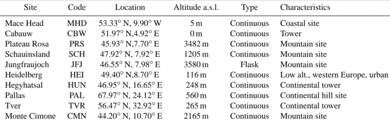
Table 3. A few site characteristics, corresponding to the included monitoring sites for atmospheric CO2. In Figs. 7, 9, 10 and 11 the
observed values are characterized as background (Obs. Bg) or non-background (Obs. NBg ) values depending on which type of air mass they are assumed to represent.
Site Code Location Altitude a.s.l. Type Characteristics Mace Head MHD 53.33◦N, 9.90◦W 5 m Continuous Coastal site Cabauw CBW 51.97◦N,4.92◦E 0 m Continuous Tower Plateau Rosa PRS 45.93◦N,7.70◦E 3482 m Continuous Mountain site Schauinsland SCH 47.92◦N, 7.92◦E 1205 m Continuous Mountain site Jungfraujoch JFJ 46.55◦N, 7.98◦E 3580 m Flask Mountain site
Heidelberg HEI 49.40◦N,8.70◦E 116 m Continuous Low alt., western Europe, urban Hegyhatsal HUN 46.95◦N, 16.65◦E 248 m Continuous Continental tower
Pallas PAL 67.97◦N, 24.12◦E 560 m Continuous Continental hill site Tver TVR 56.47◦N, 32.92◦E 265 m Continuous Continental tower Monte Cimone CMN 44.20◦N, 10.70◦E 2165 m Continuous Mountain site
In July all models predict the same fossil CO2
contribu-tion (±1 ppm) across Europe, except at Heidelberg where the difference in-between models again is large and the ob-served levels are overestimated except by the LMDZ model. This overestimation could indicate that the included fossil fuel emissions are too large in this region in summer.
In December the simulated biospheric CO2component is
generally higher in the interior of the continent than close to the coast. This is because respiratory CO2 is
progres-sively accumulating along the main air-flow directed on av-erage from the Atlantic to the continent. In July, day-time biotic CO2is lower over land due to photosynthesis.
Excep-tions are the alpine high-altitude sites Plateau Rosa (PRS) and Jungfraujoch (JFJ) where CO2respired during previous
nights can be uplifted by daytime convective mixing, leading to a positive CO2signal compared to Mace Head. At most
sites a larger spread amongst the models is generally seen for the biotic signal compared to the other CO2components, and
this spread is enhanced during summer. This is a reflection of different strengths of the diurnal mixing in the models (see also Fig. 2).
The modelled oceanic component of CO2shows a weaker
signal and less spread than the other components both dur-ing summer and winter (note the differences in the scales in Fig. 4). Relatively small longitudinal gradients (<2.5 ppm) are seen for this component and the gradient tend to be most pronounced in LMDZ in July. In December the correspond-ing gradients are quite similar in the model results.
In December the West-East gradient of the total CO2
sig-nal across the stations is captured within ±4 ppm at three (PRS, SCH, PAL) out of five stations with observations, while the high levels at HEI and HUN are underestimated by nearly all models. In contrast, most models underestimate the negative CO2difference between the Mace Head and central
and northern regions of Europe (e.g. the Finnish station Pal-las (PAL)) in July. Based on the evaluation of222Rn (see Ver-meulen et al., in preparation) and the fossil fuel component,
we attribute this bias to the NEE component. The maximum drawdown in the TURC NEE fluxes occurs about one month too early and the uptake in July is thereby underestimated. By assuming that the biosphere is in balance on a yearly ba-sis (see Sect. 2.2), we also neglect the terrestrial sink of the Northern Hemisphere, which may lead to an underestimation of the biospheric summer uptake and hence could explain the simulated underestimation of the westward depletion of CO2
across Europe.
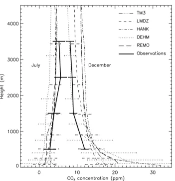
4.2 Vertical profiles of CO2through July and December
Vertical CO2profile observations from Orleans, France
pro-vide a constraint on model simulation of vertical air ex-change. The observations are from approximately weekly sampled flasks filled onboard an aircraft at 500, 1500, 2500 and 3500 m above ground The observations are taken dur-ing fair weather conditions around mid-day. We selected the model output for afternoon concentrations, but not for fair weather conditions. An arbitrary reference value of 360 ppm is subtracted from the observations. Figure 5 shows that the observed CO2increases with height during summer and
de-creases with height during winter. All the models capture qualitatively these gradients, but the modeled summer-winter contrast tends to be too large.
The figure shows that below 500 m, and hence below the lowest observation level, the models diverge strongly. Higher resolution models predict considerably higher concentrations at the surface in winter compared to the coarser resolution global models. The error bars show the monthly standard deviation for one regional model (DEHM) and one global model (LMDZ). They indicate that the variability of regional models increases greatly closer to the surface compared to global models, in accordance with the time series evaluation discussed in the following.
Fig. 5. Monthly mean observed and simulated vertical profiles for
July and December at Orleans (48.83◦N, 2.50◦E), France. The ob-served curves are based on weekly flask measurements sampled on-board an aircraft and then averaged at 500, 1500, 2500 and 3500 m above ground. A value of 360 ppm has been subtracted from the observations. The simulated curves are based on daytime values. Error bars are shown for the observations as well as for the DEHM and LMDZ model in order to display the standard deviation of the predicted concentrations at the different heights.
5 Results: time series and statistical evaluation
Due to local sources, variations in PBL depth and topo-graphic characteristics, the observations at a given station may not be spatially representative of an area large enough to be comparable to the resolution of the models. As shown by Gerbig et al. (2003) this representation error increases sig-nificantly with the horizontal averaging distance (or model grid size). This is important to bear in mind, in the following data-model comparisons including continuous data on land (see the list of stations in Table 3).
For the comparisons each model output has been sampled at each station and averaged on an hourly basis. In the ver-tical, modeled concentrations are linearly interpolated to the station altitudes.
5.1 Time series for July
During July, the uptake of CO2 as well as the diurnal PBL
height are close to their annual maximum over Europe. An important question is to what extent models differ among each other for representing the diurnal cycle of CO2 which
dominates the short-term variability. For all stations, models
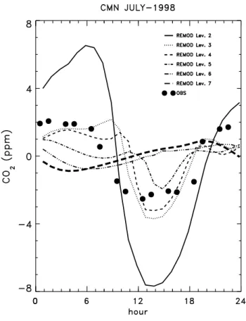
Fig. 6. Observed and simulated mean diurnal cycle (UTC) at four
monitoring sites in Europe (see Table 3 for a short description of the different sites). Based on hourly values from July and December 1998.
show a common tendency to underestimate the amplitude of the CO2diurnal cycle. We illustrate this in Fig. 6 by
com-paring the predicted and observed mean diurnal cycle at two mid- to high-elevation mountain stations (SCH and CMN; resp. at 1205 m a.s.l. and 2165 m a.s.l.) and two lower eleva-tion staeleva-tions (HUN and PAL; resp. in Western Hungary and Northern Finland). The Hungarian station is a tower with measurements from four levels. Here we include the data from the 115 m level, as the lower levels are more sensitive to local sources that are not well represented in the model grids used in this study.
Both HUN and PAL sites in Fig. 6 show a large spread amongst models for the diurnal amplitude of CO2, ranging
from 18 to 45 ppm at HUN (observed amplitude is ∼60 ppm) and from 1 to 9 ppm at PAL (observed amplitude is ∼7 ppm). All models produce an increase in concentration starting at sunset when PBL convection stops, and lasting until photo-synthesis begins again in the next morning at around 07:00
to 08:00 LST. At the Hungarian site (HUN), all models are nicely in phase with observations, but REMO, DEHM and HANK underestimate the diurnal amplitude by a fac-tor of 1.2 to 1.5, while LMDZ and TM3 underestimate it by roughly a factor of 3. At Pallas (PAL) the difference be-tween mesoscale models and global models is less clear. In general the models underestimate the observed diurnal cycle by a factor of ∼2–7. This is not surprising since the pre-scribed TURC flux (see Sect. 2.2) is known to underestimate the NEE diurnal cycle amplitude at high latitudes compared to eddy-flux tower measurements (Aalto et al., 2004).
The CO2diurnal variation reflects the day-night contrast
both in NEE and in PBL vertical mixing and its variability. As the same set of surface fluxes are being used in all the models, differences between models must reflect differences in vertical/horizontal mixing. The importance of the vertical resolution within the PBL is evident in the LMDZ simula-tions at the low altitude site HUN, where the diurnal cycle is underestimated. Over Europe the horizontal resolution is about the same as in HANK, but the vertical resolution of the PBL is lower (4 levels below 1500 m against 10 i HANK) and the parametrization of turbulent diffusion is different. For TM3 the coarser horizontal resolution of the fluxes can be part of the explanation for the smooth diurnal signal seen for this model.
Besides the biosphere-atmosphere exchange fluxes diurnal changes in vertical mixing also cause a diurnal variation in the fossil fuel component, on the order of up to 3 ppm at low altitude stations close to regional fossil emissions, like HUN. In contrast, diurnal vertical mixing acting on the oceanic CO2 component contributes negligibly to the observed
sig-nals (e.g. <0.1 ppm at HUN).
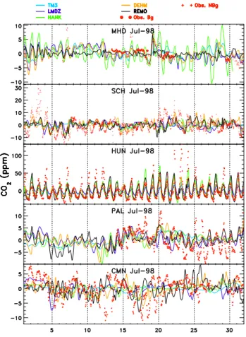
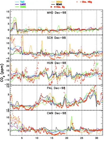
Figure 7 illustrates the hourly variability of CO2
through-out the month of July. It is seen again that none of the mod-els are able to reproduce the very high CO2 mixing ratios
observed during some nights for the same reasons discussed earlier on.
At mountain stations SCH and CMN, all models simulate diurnal cycles in CO2in July as for lower altitude sites, but
smaller in amplitude with 0.5 to 7 ppm for SCH and 0.5 to 2.5 ppm for CMN (Figs. 6 and 7). The timing of the diur-nal cycle is shifted by a few hours compared to low eleva-tion staeleva-tions, with both an earlier nighttime maximum and daytime minimum. As seen in both Figures the models un-derestimate the observed amplitude of the diurnal cycle at CMN (∼4.5 ppm) and SCH (∼7 ppm), and are out of phase with the observations. At CMN, all models are opposite in phase with the observations, producing a maximum of CO2
at mid-day. We attribute such deviations to the fact that the mountain stations in the real world are more directly con-nected to surface sources by local thermally-induced circula-tions (upslope winds over sunlit slopes) during the day than predicted in a model with smooth topography. In the cur-rent study we also sample the model output at the elevation (a.s.l.) corresponding to the actual elevation of each site, i.e.
Fig. 7. Observed and simulated hourly time series for July 1998. At
five different monitoring sites in Europe (see Table 3).
at some higher model level. Therefore, in most mountain re-gions the CO2signal at a given station is in the models more
decoupled from the ground than in reality because the real elevation of the site is much higher than the model topogra-phy. The lagged predicted diurnal signal is then induced by the diurnal cycle at the surface propagating up through the convective PBL in the model. An exemplification of this ef-fect can be seen in Fig. 8 where the observed diurnal cycle at CMN (2165 m a.s.l.) is compared to the REMO output for July. When plotting the CO2values at several model layers,
it is clear that the values at the model layer corresponding to the true height of the station (the sixth layer at 1743 m a.s.l.) is out of phase with the observed diurnal cycle. The agree-ment between model predictions and observations increases closer to the surface and the results from the fourth model layer (1090 m a.s.l. and 529 m above ground) captures the diurnal cycle much better. It is thus apparent that represen-tation of mountain srepresen-tations is an important issue that needs to be addressed, when such data are included in atmospheric inversions (e.g. Peylin et al., 2005).
The hourly data shown in Fig. 7, nevertheless indicate that the models are able to capture most of the synoptic scale
Fig. 8. Mean diurnal cycle for July as simulated by the REMO model and observed at the mountain site Monte Cimone (2165 m a.s.l.) in Italy. The model results are shown for the lowest six levels just above the surface layer.
variability leading e.g. to day-to-day changes in the ampli-tude of the diurnal cycle. These changes are mainly caused by synoptic variability in atmospheric transport processes coupled with synoptic changes in NEE. As an example, for the night of 7–8 July at the low altitude Hungarian station (HUN), there was no observed build up of CO2after two
con-secutive nights with high CO2accumulations. This “event”
correctly reproduced in all models is explained by the pas-sage of a front during 7–9 July that broke down the stability of the nocturnal PBL.
However, the large differences between models at the hourly time scale suggest to average the measurements, for instance over the mid-day period, when convection is (gen-erally) well developed and the CO2variability is small. The
new question raised here is then the ability and robustness of transport models to capture the to-day changes in day-time CO2, related to transport on synoptic time scales and
containing information on the underlying source/sink pro-cesses. We show in Fig. 9 the day-time (10:00–17:00 LST) averaged data and model results at five stations (Table 3). Overall, all models capture the timing of most day-to-day changes, but they still show significant differences in the
pre-Fig. 9. Daily averaged time series based on daytime selected values
in July 1998.
dicted magnitude. This suggests that while horizontal syn-optic transport is realistic and similar both using mesoscale and global models the vertical transport is markedly different among the models.
Each station also has specific characteristics, which can be used to constrain different aspects of the transport models. The CO2record at Mace Head shows very stable (±0.3 ppm)
marine “baseline” CO2 values under westerly wind
condi-tions (13–18 July except 16 July, in Fig. 9) when reached by oceanic air masses, over which continental air masses de-liver CO2maxima and minima (Bousquet et al., 1997). This
is fairly well reproduced in most of the models, but with a larger amplitude (±0.5 to ±1.0 ppm). At the continental lo-cation in Central Europe (HUN) a larger observed and mod-elled CO2 variability (by a factor of around 2) caused by
synoptic systems is seen compared to mountain or coastal stations. All models roughly capture this feature.
5.2 Time series for December
The averaged diurnal cycle, hourly time series and daytime selected means for December are displayed in Figs. 6, 10 and 11, respectively. In general, on an hourly basis, the
Fig. 10. Observed and simulated hourly time series for December
1998.
agreement between models and between models and obser-vations is much higher in December compared to July. Out-side the photosynthetically active period, soils in temperate and northern Europe respire CO2almost uniformly
through-out the day, resulting in a small biospheric CO2diurnal
cy-cle (e.g. Aurela et al., 2001). Further south, where photo-synthesis persists, the amplitude of the diurnal NEE is also smaller than in summer (e.g. Kowalski et al., 2003). Gen-erally, low-pressure systems are more frequent and intense in winter than in summer due to the larger temperature con-trasts between the continents and the ocean. They form over the North Atlantic before they move in a westerly flow over the continent each 3–5 days. Besides, as seen in Figs. 1 and 4, day-time mixing is inhibited in December, which has the effect to accumulate CO2in the boundary layer (e.g. Levin et
al., 1995; Haszpra, 1999), a phenomenon also observed for other anthropogenic pollutants.
We note the occurrence at HUN of periods of a few days during which CO2is very high (10 to 20 ppm above the
ma-rine background). This station is located in the Carpathian Basin, surrounded by a ring of mountains. Anticyclonic con-ditions can during winter lead to trapping of cold air in this basin and hence very high surface concentrations of CO2.
Fig. 11. Daily averaged time series based on daytime selected
val-ues in December 1998.
Likewise, two periods with a gradual near surface CO2
accu-mulation of about 5–10 ppm within 2–4 days is observed at PAL in Finland. At MHD, there is one “pollution” episode of European origin with CO2 rising by up to about 8 ppm
above the marine baseline in early December. This episode is associated with a high pressure system developed just west of Ireland. Also at the more high elevation sites (CMN and SCH) episodes with CO2levels above 10 ppm are seen
dur-ing December.
5.3 Statistical evaluation
In order to obtain a more quantitative measure of the models’ ability to capture the observed variability, a statistical evalua-tion is carried out at five European sites. So-called Taylor di-agrams (Taylor, 2001), displaying both relative standard de-viation, relative root-mean-square difference and the corre-lation between observed and simulated time series, are used here. These statistics can be used to highlight how much of the overall root-mean-square difference is related to differ-ences in variance and how much is due to poor correlation between models and observations. In the Taylor diagram, the relative standard deviation, defined as the simulated standard
Fig. 12. Taylor diagram collecting the relative standard deviation,
relative RMS difference and the correlation coefficient between ob-served and simulated time series of CO2during the month of July
and December 1998. The statistics are based on hourly data from five European locations and the five models. For HANK the result at MHD is off the scale with a relative standard deviation of 2.22 and a correlation coefficient of 0.77.
deviation along time divided by the observed one, is plotted as radial distance from the origin. The cosine of the angle with respect to the horizontal axis equals the correlation co-efficient. A (hypothetical) model in perfect agreement with observations would be located where the circle with radius equal to unity intersect the x-axis (indicated as a star in the plot). The Taylor diagram has the property that the distance between an actual model result and the reference point of the perfect model (the star) equals the relative root mean square error (RMS). In Fig. 12, Taylor diagrams have been calcu-lated from all hourly data, while Fig. 13 is calcucalcu-lated from
Fig. 13. Taylor diagram collecting the relative standard deviation,
relative RMS difference and the correlation coefficient between ob-served and simulated time series of CO2during the month of July
and December 1998. The statistics are based on daily mean values based on daytime selected data from five European locations and the five models. For HANK the result at MHD is off the scale with a relative standard deviation of 2.81 and a correlation coefficient of 0.79. The same is true for DEHM at MHD/PRS with a standard deviation of 2.07/2.09 and a correlation of 0.78/0.85.
daily mean concentrations based on day-time selected val-ues.
Comparing the statistics of hourly data (strongly influ-enced by the diurnal cycle, at least in summer) and of day-time selected daily means (expected to reflect synoptic vari-ability), the picture turns out to be broadly similar. Mod-elled standard deviations are generally larger for the daily means, in particular at the coastal site Mace Head (MHD) and the mountain site Plateau Rosa (PRS). Correlation
coefficients are similar between hourly and daily for most stations/models.
As expected from the time series analysis above, all the models underestimate the variability during summer, with a tendency towards smaller normalized standard deviation for coarser-resolution models. Plateau Rosa (PRS) and Schauinsland (SCH) often show poorer correlations than the other sites, in accordance with the before-mentioned difficul-ties for properly locating mountain sites in models.
In December, when diurnal cycles are small, the model-data correlations are slightly higher than in July, as the phase of the synoptic variability is reasonably captured by all mod-els. However, the size of individual high CO2 events is
mostly still underestimated, especially by the two global models, and by REMO (the latter maybe because of the use of boundary conditions based on simulations with the global model TM3). Nevertheless, overestimation occurs as well. When compared to observations, the DEHM model shows a high correlation (>0.65) at four sites as well as a relative standard deviation around one and a small RMS. The stan-dard deviation of HANK is also reasonable for MHD and HUN, while it is greatly underestimated at the mountain sta-tions PRS and SCH.
6 Summary and conclusions
We have tested model behavior for simulating lower tropo-spheric CO2 across Europe using one set of surface fluxes
and five atmospheric transport models with different hori-zontal and vertical resolution. Model predictions are con-fronted with new continuous and discrete CO2 and14CO2
atmospheric concentrations measured for the purpose of es-timating the carbon balance of Europe using an atmospheric approach. A main purpose of the study is to learn how to combine continental data and models for flux estimation pur-pose given the complex nature of lower troposphere CO2
above the continents. The results show that the spread of predicted CO2across the models is large (up to 10 ppm for
the monthly mean distribution). From the separated compo-nents (biosphere, ocean and fossil fuel) it is evident that these differences are not only linked to the horizontal resolution of the models, but also to a large degree to the representation of mixing within the boundary layer and the vertical resolution of the models. The spread is reduced when restricting sam-pling to the afternoon. It is further reduced when samsam-pling a few hundred meters above ground.
Main conclusions and recommendations resulting from the study for constraining land carbon sources and sinks us-ing high-resolution concentration data and state-of-the art transport models through inverse methods are given in the following:
1) At altitude stations both coarse and high-resolution models employed fail to reproduce phasing of daily cycles as well as absolute concentrations observed due
to an insufficient representation of the surface topography. Furthermore, the flow fields around mountainous sites are ex-tremely difficult to simulate and therefore the transport pat-terns from the source areas to the mountain site are difficult to catch. The recommendation is therefore that low altitude stations presently are preferable in inverse studies. If high altitude stations are used then the model level that represents the specific sites should be applied.
2) The modelled height of the PBL has substantial influ-ence on the concentration levels. This parameter is never-theless very difficult to simulate correctly and this is one of the main sources of uncertainties in transport models. The model-surface data comparisons show a large spread, with the observed diurnal cycle being underestimated by up to a factor of 1.5 for the regional models and up to a factor of 3 for global models at a low altitude continental site in Hungary. Especially during night time the height of the PBL can be uncertain with several hundred percent, and from the hourly time series it is evident that the models underestimate the night-time concentrations. During day time the PBL height is better resolved by the models and hence less uncertain. Fur-thermore the parameterizations of the PBL height are mainly designed for day time applications. The recommendation is therefore that at low altitude sites only the afternoon values of concentrations can be represented sufficiently well by current models and therefore afternoon values are more appropriate for constraining large-scale sources and sinks in combination with transport models.
3) The vertical CO2profile is difficult to simulate,
espe-cially near the ground due to the surface exchange. Even when using only afternoon values it is clear that data sam-pled several hundred meters above ground can be represented substantially more robust in the models. The recommenda-tion is therefore to emphasize the use of tower data in inverse studies.
4) The traditional coarse resolution transport models are too coarse to resolve not only fine-scale features associated with fossil fuel emissions, but also larger-scale features like the concentration distribution above the south-western Eu-rope. Our results indicate that a horizontal resolution of max. 1◦×1◦ combined with a vertical resolution of max. 100 m for the lowest layer, should be able to capture such distribu-tions. The recommendation is therefore to use higher resolu-tion models in future studies including continental data.
It is important to note that both high altitude sites and hourly data in general include important information about the carbon cycle that could be valuable in budget studies. But in order to include such data in studies with the current gener-ation models a detailed assessment of model capability needs to be carried out for each site, preferable in cooperation with the people responsible for the monitoring network.
Acknowledgements. The work has been done within the
frame-work of the EU cluster project CARBOEUROPE, sub-project AEROCARB (Airborne European Regional Observations of the
Carbon Balance). We thank the participants of AEROCARB for useful discussions and for making their observations available for this study. Especially warm thanks to I. Levin for her thoughtful comments to this work. The project was funded by the European Commission under contract no. EVK2-CT-1999-00013.
Edited by: W. E. Asher
References
Aalto, T., Hatakka, J., Paatero, J., Tuovinen, J.-P., Aurela, M., Lau-rila, T., Holm´en, K., Trivett, N., and Viisanen, Y.: Tropospheric carbon dioxide concentrations at a northern boreal site in Fin-land: basic variations and source areas, Tellus, 54B, 110–126, 2002.
Aalto, T., Ciais, P., Chevillard, A., and Moulin, C.: Optimal de-termination of the parameters controlling biospheric CO2fluxes over Europe using eddy covariance fluxes and NDVI measure-ments, Tellus, 56B, 93–104, 2004.
Apadula, F., Gotti, A., Pigini, A., Longhetto, A., Rocchetti, F., Cas-sardo, C., Ferrarese, S., and Forza, R.: Localization of source and sink regions of carbon dioxide through the method of the syn-optic air trajectory statistics, Atmos. Environ., 37, 3757–3770, 2003.
Aurela, M., Laurila, T., and Touvinen, J.-P.: Seasonal CO2balances
of a subarctic mire, J. Geophys. Res., 106, 1623–1637. Bakwin, P. S., Tans, P. P., Hurst, D. F., and Zhao, C.:
Mea-surements of carbon dioxide on very tall towers: results of the NOAA/CMDL program, Tellus, 50B, 401–415, 1998.
Blasing T. J., Broniak, C. T., Marland, G.: The annual cycle of fossil-fuel carbon dioxide emissions in the United States, Tellus, 57B, 107–115, 2005.
Bousquet, P., Ciais, P., Monfray, P., Balkanski, Y., and Ramonet, M.: Influence of two atmospheric transport models on inferring sources and sinks of atmospheric CO2, Tellus, 48B, 568–582, 1996.
Bousquet, P., Gaudry, A., Ciais, P., Kazan, V. P., Monfray, P., Sim-monds, P. G., Jennings, S. G., and O’Connor, T. C.: Atmospheric concentration variations recorded at Mace Head, Ireland from 1992 to 1994, Phys. Chem. Earth, 21, 5-6, 477–481, 1997. Bousquet, P., Peylin, P. Ciais, P., Le Qu´er´e, C., Friedlingstein, P.,
and Tans, P. P.: Regional changes in carbon dioxide fluxes of land and oceans since 1980, Science, 260, 1342–1346, 2000. Chevillard, A.: Etude a haute resolution du CO2atmospherique en
Europe et en Siberie, Impact pour les bilans de carbone, PhD Thesis, Universite Pierre et Marie Curie, Paris, France, 2001. Chevillard, A., Ciais, P., Karstens, U., Heimann, M., Schmidt, M.,
Levin, I., Jacob, D., and Podzun, R.: Transport of222Rn using the regional model REMO, A detailed comparison with measure-ments over Europe, Tellus, 54B, 872–894, 2002a.
Chevillard A., Karstens, U., Ciais, P., Lafont, S., and Heimann, M.: Simulation of atmospheric CO2over Europe and Western Siberia
using the regional scale model REMO, Tellus, 54B, 872–894, 2002b.
Christensen, J. H.: The Danish Eulerian hemispheric model - a three-dimensional air pollution model used for the arctic, At-mos. Environ., 31, 4169–4191, 1997.
Christensen, J., Brandt, J., Frohn, L. M., and Skov, H.: Modelling of Mercury in the Arctic with the Danish Eulerian Hemispheric
Model, Atmos. Chem. Phys., 4, 2251–2257, 2004, http://www.atmos-chem-phys.net/4/2251/2004/.
Denning, A. S., Randall, D. A., Collatz, G. J., and Sellers, P. J.: Simulations of terrestrial carbon metabolism and atmospheric CO2in a general circulation model, Part 2: Simulated CO2
con-centrations, Tellus, 48B, 8543–8567, 1996.
Fan S., Gloor, M., Mahlman, J., Pacala, S., Sarmiento, J., Takahashi T., and Tans, P.: A large terrestrial carbon sink in North Amer-ica implied by atmospheric and oceanic carbon dioxide data and models, Science, 282, 442–446, 1998.
Frohn, L. M., Christensen, J. H., and Brandt J.: Development of a high resolution nested air pollution model – the numerical ap-proach, J. Comput. Phys., 179(1), 68–94, 2002.
Frohn, L. M.: A study of long-term high-resolution air pollution modelling, PhD thesis, National Environmental Research Insti-tute, Department of Atmospheric Environment, Denmark, 2004. Fung, I. Y., Tucker, C. J., and Prentice, K. C.: Application of advanced very high resolution radiometer vegetation index to study atmosphere-biosphere exchange of CO2, J. Geophys. Res., 92(D3), 2999–3015, 1987.
Geels, C.: Simulating the current CO2content of the atmosphere:
Including surface fluxes and transport across the Northern Hemi-sphere, PhD thesis, National Environmental Research Institute, Department of Atmospheric Environment, Denmark, 2003. Geels, C., Doney, S. C., Dargaville, R., Brandt J., and Christensen,
J. H.: Investigating the sources of synoptic variability in atmo-spheric CO2measurements over the Northern Hemisphere
con-tinents – a regional model study, Tellus, 56B, 35–50, 2004. Gerbig, C., Lin, J. C, Wofsy, S. C., Daube, B. C., Andrews,
A. E., Stephens, B. B., Bakwin, P. S., and Grainger, C. A.: Towards constraining regional-scale fluxes of CO2 with
atmo-spheric observations over a continent: 1. Observed spatial vari-ability from airborne platforms, J. Geophys. Res., 108(D24), 4756, doi:10.1029/2002JD003018, 2003.
Gloor, M., Fung, S. M., and Sarmiento, J.: Optimal sampling of the atmosphere for purpose of inverse modeling: A model study, Global Biogeochem. Cycles, 14(1), 407–428, 2000.
Grell, G. A., Dudhia, J., and Stauffer, D. R.: A Description of the Fifth-Generation Penn State/NCAR Mesoscale Model (MM5). NCAR/TN-398+STR, NCAR Technical Note, Mesoscale and Microscale Meteorology Division, National Center for Atmo-spheric Research, Boulder, Colorado, pp. 122, June 1995. Gurney, K. R., Law, R. M., Denning, A. S., Rayner, P. J., Baker,
D., Bousquet, P., Bruhwiler, L., Chen, Y.-H., Ciais, P., Fan, S., Fung, I. Y., Gloor, M., Heimann, M., Higuchi, K., John, J., Maki, T., Maksyutov, S., Masari, K., Peylin, P., Prather, M., Pak, B. C., Randerson, J., Sarmiento, J., Taguchi, S., Takahashi T., and Yuen, C.-W.: Towards robust regional estimates of CO2sources
and sinks using atmospheric transport models, Nature, 415, 626– 630, 2002.
Gurney, K. R., Law, R. M., Denning, A. S., Rayner, P. J., Baker, D., Bousquet, P., Bruhwiler, L., Chen, Y.-H., Ciais, P., Fan, S., Fung, I. Y., Gloor, M., Heimann, M., Higuchi, K., John, J., Kowal-czyk, E., Maki, T., Maksyutov, S., Peylin, P., Prather, M., Pak, B. C., Sarmiento, J., Taguchi, S., Takahashi T., and Yuen, C.-W.: TransCom 3 CO2 inversion intercomparison: 1. Annual mean
control results and sensitivity to transport and prior flux informa-tion, Tellus, 55B, 555–579, 2003.