Fully nonlinear features of the energetic beam-driven instability

HAL Id: hal-01722771

https://hal.archives-ouvertes.fr/hal-01722771

Submitted on 5 Mar 2018

HAL is a multi-disciplinary open access

archive for the deposit and dissemination of

sci-entific research documents, whether they are

pub-lished or not. The documents may come from

teaching and research institutions in France or

abroad, or from public or private research centers.

L’archive ouverte pluridisciplinaire HAL, est

destinée au dépôt et à la diffusion de documents

scientifiques de niveau recherche, publiés ou non,

émanant des établissements d’enseignement et de

recherche français ou étrangers, des laboratoires

publics ou privés.

instability

M. Lesur, Y. Idomura, X. Garbet

To cite this version:

M. Lesur, Y. Idomura, X. Garbet. Fully nonlinear features of the energetic beam-driven instability.

Physics of Plasmas, American Institute of Physics, 2009, 16 (9), �10.1063/1.3234249�. �hal-01722771�

Fully nonlinear features of the energetic beam-driven instability

M. Lesur,1,2Y. Idomura,1and X. Garbet2

1

Japan Atomic Energy Agency, Higashi-Ueno 6-9-3, Taitou, Tokyo 110-0015, Japan

2

Commissariat à l’Energie Atomique, IRFM, F-13108 Saint Paul Lez Durance, France

共Received 27 May 2009; accepted 27 August 2009; published online 25 September 2009兲 The so-called Berk–Breizman model is applied to a cold bulk, weak warm beam, one-dimensional plasma, to investigate the kinetic instability arising from the resonance of a single electrostatic wave with an energetic particle beam. A Vlasov code is developed to solve the initial value problem for the full-f distribution, and the nonlinear evolution is categorized in the whole parameter space as damped, steady-state, periodic, chaotic, or chirping. The saturation level of steady-state solutions and the bifurcation between steady-state and periodic solutions near marginal stability match analytic predictions. The limit of a perturbative numerical approach when the resonant region extends into the bulk is shown. Frequency sweeping is observed, with time-evolution approaching theoretical results. A new method to extract the dissipation rate from frequency diagnostics is proposed. For small collision rates, instabilities are observed in the linearly barely stable region. © 2009 American Institute of Physics.关doi:10.1063/1.3234249兴

I. INTRODUCTION

Containment of the energy of alpha particles is critical to achieve break even in magnetically confined fusion devices. In an ignited tokamak, these highly energetic particles can give birth to Alfvén wave instabilities in the form of isolated single modes. A concern is that these instabilities may lead to the premature ejection of the energetic population before they could give their energy to the core to sustain the reac-tion. In general, energetic particle driven instabilities are de-scribed in a three-dimensional共3D兲 configuration. However, near the resonant surface, it is possible to obtain a new set of variables in which the plasma is described by a one-dimensional 共1D兲 Hamiltonian in two conjugated variables,1–4if we assume that a single resonance dominates. In this sense, there is a whole class of beam injection prob-lems that are homothetic to a simple 1D single mode bump-on-tail instability. Observed quantitative similarities1,5 be-tween this class of beam instabilities and the so-called Berk– Breizman共BB兲 problem3,4,6 are an indication of the validity of this reduction of dimensionality. This analogy enables more understanding of a fully nonlinear problem in a com-plex geometry by using a model that is analytically and nu-merically tractable, as a complementary approach to heavier 3D analysis. From these backgrounds, we investigate the ki-netic features of the self-consistent interactions between an energetic particle beam and a weakly unstable electrostatic wave in 1D plasma.

The BB problem is an augmentation of the Vlasov– Maxwell system, where we take into account a collision term that represents particle annihilation and injection processes at a rate␯a, and an external wave damping accounting for

back-ground dissipative mechanisms at a rate ␥d. In this system,

we consider a bump-on-tail velocity distribution comprising a Maxwellian bulk and a beam of energetic particles, and we apply a small electrostatic perturbation. Depending on the parameters of the system, the perturbation may be damped or amplified due to the transfer of energy between resonant

par-ticles and the wave. In the unstable case, when the perturba-tion is small, the linear theory predicts exponential growth of the wave amplitude. Then the trapping of resonant particles significantly modify the distribution function and an island structure appears. The saturation of the instability and the following nonlinear evolutions are determined by a compe-tition among the drive by resonant particles, the external damping, the particle relaxation which tends to recover the initial positive slope in the distribution function, and particle trapping that tends to smooth it. It has been predicted3,4,6and observed7 that three kinds of behaviors emerge, namely, steady-state, periodic, or chaotic responses, depending on the strength of each factor. In addition, chaotic solutions can display shifting of the mode frequency共chirping兲, both up-wardly and downup-wardly, as pairs of hole and clump are formed in the distribution.8–10

On the one hand, theories have been developed by Berk et al.6,8–11to predict the quantitative behavior of such insta-bilities in various parameter regimes and explain underlying mechanisms. The validity of some of these theories has been tested by numerical simulations based on a reduced model solving only resonant particles with adiabatic and cold bulk plasmas. A concern with this perturbative approach is that, as the instability grows, the resonant region may expand includ-ing a significant portion of bulk particles, and when chirpinclud-ing occurs, the resonant point may propagate into the bulk. In such situations, kinetic effects of the bulk plasma should also be taken into account. On the other hand, numerical simula-tions of the full distribution kinetics共full-f兲 have been per-formed by Vann et al.7in the whole共␥d,␯a兲 parameter space.

However, in general, this approach shows some difficulty in simulating situations considered in the aforementioned theo-ries, which assume a plasma near marginal stability with a cold bulk and a weak beam, and therefore, these theories have not been validated with this approach. To simulate such a situation, we need a robust and accurate numerical scheme. The aim of this paper is to fill the gap between these two

fronts of the current state of research, with quantitative com-parisons between available theory and nonreduced kinetic simulations. For this purpose, we develop a full-f Vlasov code based on the constrained interpolation profile-conservative semi-Lagrangian共CIP-CSL兲 scheme12for solv-ing this initial value problem. We recall the equations of the BB model, present the main principles of our code, which will be referred to as BB-solver, and the equations of the reduced model in Sec. II. A first verification of the BB-solver consists of confirming its capability to solve the simpler Vlasov–Poisson system by recovering the saturation level, relative oscillation amplitude, and the so-called Bernstein– Greene–Kruskal 共BGK兲 steady-state solution13 in the colli-sionless limit without external damping. Then, we analyze the convergence and conservation properties of the BB-solver for a system with finite␥d and␯a, and benchmark it

against a parameter scan given in former works by Vann.7 Compared to this benchmark, our choice of parameters for testing the theory constitutes difficult conditions for numeri-cal stability and drastinumeri-cally increases a computational cost. As a consequence, we must take special care in choosing an advection scheme that minimizes the computation time. Therefore a discussion of the relevancy of the CIP-CSL ad-vection scheme and a comparison with four other adad-vection schemes are provided in Sec. III. Armed with a verified set of numerical tools, we then proceed to the investigation of the validity of available theory. We apply the BB-solver to a distribution function comprising a cold bulk and a weak warm beam, and perform a systematic parameter scan in 共␥d,␯a兲. The categorization of the nonlinear behavior of each

solution is presented in the behavior bifurcation diagram of Sec. IV. In the whole parameter space, we observe a quanti-tative agreement between the numerical solution and analytic predictions for the linear growth rate. We validate the ana-lytic theories for the following nonlinear features: saturation level in the parameter regime above marginal stability, satu-ration level and bifurcation criterion between steady-state and periodic solutions near marginal stability, and time-evolution of a frequency shifting mode. In this study, we compare our numerical results also with similar previous computations based on the reduced model, to show the limits of such model.

II. PHYSICAL AND NUMERICAL MODEL A. The Berk–Breizman model

We cast the so-called BB model14 as follows. We con-sider a 1D plasma with a distribution function f共x,v,t兲. To ensure charge neutrality, we assume a background population of the opposite charge with a distribution function f¯共v,t兲, the space average of f. In the initial condition, the velocity distribution,

f0共v兲 ⬅ f¯共v,t = 0兲 = f0

P_{共v兲 + f}

0

B_{共v兲, 共1兲}

comprises a Maxwellian bulk,

f₀P共v兲 = nP vP

冑

2␲

e−1/2共v/vP兲2_, 共2兲

and a beam of high-energy particles,

f₀B共v兲 = nB vB

冑

2␲

e−1/2共v − v0/vB兲2_, 共3兲

where nPand nBare bulk and beam densities,vPandvB are

thermal velocities of bulk and beam particles, andv0 is the

beam drift velocity.

The evolution of the electronic distribution is given by the kinetic equation

⳵f ⳵t +v ⳵f ⳵x+ qE m ⳵f ⳵v= −␯a共v兲共f − f0兲, 共4兲 where q is the charge, m is the mass, and E is the electric field. Here, collisions are taken into account in the form of a Krook operator15 that is a model for both source and sink of energetic particles that tend to recover the initial distribution at a rate␯a. If we assume cold and adiabatic bulk plasmas,

␯a共v兲 acts only on the beam. Reflecting this situation, we

design the velocity dependency of␯a共v兲 as

␯a共v兲 =

再

␯a if v⬎ v␯,

0 else,

冎

共5兲

with v_␯ satisfying fP共v␯兲/ fP共0兲=⑀␯, and we choose

⑀␯= 0.001. Hence, ␯a共v兲 is constant in the beam region and

zero in the bulk region, except for the benchmark in Sec. III D where it is explicitly stated to be constant everywhere.

In the expression of the electric field, E共x,t兲 = Eˆk共t兲e

ıkx

+ c.c., 共6兲

we assume a single mode of wave number k, reflecting the situation of a low toroidal mode number Alfvèn eigenmode, whose excited spectrum is usually discrete. The displacement current equation,

⳵E

⳵t = − 4␲q

冕

v共f − f¯兲dv − 2␥dE, 共7兲 yields the time evolution of the wave. The initial condition is given by solving Poisson’s equation. In Eq.共7兲, an external wave damping has been added to model all linear dissipation mechanisms of the wave energy to the background plasma, which are not included in the previous equations. The factor 2 in front of␥d has been chosen for the sake of simplicity

and consistency with Berk and Breizman’s literature. In the collisionless limit, if we assume a small perturbation and a linear growth rate␥much smaller than the real frequency␻, linear calculations yield the relation

␥=␥L−

2␥d

␻

冏

⳵R共D_⳵⍀L兲

冏

⍀=␻

, 共8兲

where␥Lis the linear growth rate in the absence of external

damping,R共DL兲=1−4␲q2/m⍀P兰v⳵vf0/kv−⍀dv, and P is

a notation for Cauchy’s principal value. In the cold Maxwell-ian limit, a simple relation,␥=␥L−␥d, stands. However, with

our choice of distribution function, we must keep in mind that there is some discrepancy between␥and␥L−␥d.

In the ideal situation, the model presented above ensures conservation of the total particle number N共t兲⬅兰fdxdv. This is proven by taking the integral over the whole phase-space of the kinetic Eq.共4兲. We get

dN

dt = −

冕

␯a共v兲共f − f0兲dxdv. 共9兲 If␯a共v兲=␯a is taken as constant, the latter equation can be

written as d⌬N

dt +␯a⌬N = 0, 共10兲

where⌬N共t兲⬅N共t兲−N共0兲. Since ⌬N共0兲=0, Eq. 共10兲 yields the total particle number conservation, d⌬N/dt=0. However, in numerical simulations, some spurious leakage of particles from the velocity boundaries induces a small error in this conservation. When␯a共v兲 has the velocity dependence of Eq.

共5兲, Eq.共10兲is changed to d⌬N

dt +␯a⌬N =␯aL

冕

−⬁

v_␯

共f¯ − f0兲dv, 共11兲

where L = 2␲/k is the system size. In the bulk part v⬍v_␯, we assume that the variation of the distribution is negligible, 共f¯共t兲− f0兲Ⰶ f0, and we show the approximative conservation

of the total particle number,

冏

d⌬N

dt +␯a⌬N

冏

Ⰶ␯aN共0兲. 共12兲

A straightforward analysis of the above model yields a power balance equation. Let us define the electric field energy density,

E共t兲 ⬅

冕

E2 8␲

dx

L . 共13兲

The power transferred from the perturbed electric field to both bulk and beam particles, not including sloshing energy, is given by

Ph共t兲 ⬅ q

冕

vEfdxdv. 共14兲

We show the power balance equation,

PE+ Ph+ Pd= 0, 共15兲

where PE⬅LdtE is the electric field power transfer, and Pd

⬅4L␥dE is the power transferred to the background plasma

by dissipative mechanisms.

B. The BB-solver

The set of Eqs. 共4兲–共7兲, describing the fully nonlinear wave-particle interaction of the BB problem, is an extension of the Vlasov–Poisson system, which is recovered in the col-lisionless共␯a= 0兲 and closed system 共␥d= 0兲 limit. In a

pre-vious work,16 we developed a 1D semi-Lagrangian Vlasov code, based on the cubic-interpolated-propagation 共CIP兲

scheme17and the splitting method,18which enabled accurate simulations of the Vlasov–Poisson system. In this work, we extend this code to include distribution relaxation and extrin-sic dissipation.

Let us now describe the algorithm of our extended Vla-sov solver or BB-solver. All quantities like f are sampled on uniform Eulerian grids with Nx and Nv grid points in the x

andv directions, respectively, within the computational do-main兵共x,v兲兩0ⱕx⬍L,vminⱕvⱕvmax其. The boundary

condi-tions are periodic in the x-direction and fixed in the v-direction. We define the Courant–Friedrichs–Lewy number CFL⬅vmax⌬tNx/2L as a measure of the time-step width ⌬t.

We use the Strang splitting19 formula to obtain a second-order accuracy in time.7 For each time step, we perform the following steps.

共1兲 Advect⳵tf +v⳵xf = 0 for a time⌬t/2.

共2兲 Solve⳵tf −␯a共v兲共f − f0兲=0 for a time ⌬t/2.

共3兲 Solve⳵tE = −4␲q兰v共f − f¯兲dv−2␥dE for a time⌬t/2.

共4兲 Advect⳵tf + qE共x兲/m⳵vf = 0 for a time⌬t.

共5兲 Repeat the step 3. 共6兲 Repeat the step 2. 共7兲 Repeat the step 1.

Numerically, steps B and B are performed by a forward Euler scheme. The remaining problem, corresponding to steps 1 and 4, is the advection of a 1D hyperbolic equation,

⳵tF + u⳵␭F = 0, 共16兲

where u is constant in the ␭ direction, ␭ is a generalized advection coordinate, and F is a general function of␭ and t. In this work, we aim at long-time accurate simulations in the whole共␥d,␯a兲 space. The choice of advection scheme is of

crucial importance to reach this goal. In Sec. III B, we show a comparison between different schemes, and from this com-parison, we chose to use the CIP-CSL scheme. The key idea is that in addition to the distribution function, we advect its integrated value␳ to keep a flux balance between neighbor-ing grids. In Appendix A, we recall the CIP-CSL algorithm for solving Eq.共16兲and its extension to the position-velocity phase-space, as presented in Ref.12.

C. Reduced model

In previous work,20 the theory of the BB problem was investigated under a perturbative approach based on a par-ticle code solving a reduced physical model.21The main hy-pothesis of this model is that the bulk particles interact adia-batically with the wave, so that their contribution to the Lagrangian can be expressed as a part of the electric field. This model describes only the time evolution of the beam part of the distribution fB. Equations 共4兲–共7兲 are then re-placed by ⳵fB ⳵t +v ⳵fB ⳵x + qE˜ m ⳵fB ⳵v = −␯a共v兲共f B − f₀B兲, 共17兲

E ˜ 共x,t兲 ⬅ E˜0共t兲sin共␰+␾兲 = mkSk q 关Q cos共␰兲 − P sin共␰兲兴, 共18兲 where␰⬅kx−␻t, dQ dt = nB

冕

Sk kf B_{共x,v,t兲cos共␰兲dxdv, 共19兲} dP dt = nB

冕

Sk kf B_{共x,v,t兲sin共␰兲dxdv, 共20兲}

where Skis a normalization constant given by

Sk

2_⬅ ␻0 3

2␲kn0

, 共21兲

where the plasma frequency is defined as␻₀2= 4␲n₀q2_{/m and}

n₀⬅兰f₀dv = nP+ nB. To be able to compare our numerical

results to previous work, we developed a reduced model Vla-sov code based on the latter set of equations.

III. CODE VERIFICATION

Throughout this article, the wave number is fixed at k = 0.3/␭D, where ␭D=vth/␻0 is the Debye length, andvth is

the thermal velocity. The linear growth rate ␥ and the real frequency␻of the wave are defined as the exact solutions of the linear dispersion relation,

␥+ 2␥d− ı␻= ␻0 2 n0

冕

⌫ v⳵vf0 共␥+␯a兲 + ı共kv −␻兲 dv, 共22兲 where⌫ is the appropriate Landau contour.22The algorithm we implemented to solve the latter equation is based on a method of residue for locating the zeros of an analytic func-tion in the complex plane.23In the following,␥Lis defined as

the exact solution of the linear dispersion relation for

␥d=␯a= 0.

A. Collisionless closed system_„␥d=␯a= 0…

As a preliminary test, let us consider the simpler colli-sionless Vlasov–Poisson model without external damping, corresponding to the model of the BB problem 共Sec. II A兲 without any particle source, sink, nor extrinsic dissipation. In the linear phase, the perturbation is much smaller than the unperturbed distribution, and the amplitude of the electric field follows an exponential growth of the bump-on-tail in-stability at a rate ␥L.

22

The linear growth goes on until the trajectories of resonant particles are significantly modified by electrostatic trapping. In the nonlinear phase, the distribution develops an island structure in phase space and becomes flat on average in the resonant velocity region. The instability saturates and the linear theory breaks down. Figure1shows the evolution of the normalized bounce frequency ␻b/␥L,

along with snapshots of the distribution function, for a cold bulk, weak warm beam initial distribution given in Sec. IV. Throughout this paper, the bounce frequency␻b of particles

that are deeply trapped in the electrostatic potential, defined as ␻b

2_⬅兩q兩kE

0/m, is used as a measure of the electric field

amplitude E0. We recover the linear growth rate obtained

from our numerical eigenvalue solver with less than 1%

er-ror. The saturation level is close to the value ␻b/␥L⬃3.2,

which was numerically obtained in Ref. 24 via a particle code with the above mentioned adiabatic cold bulk reduced model.

In the time-asymptotic limit, the steady-state solution of the Vlasov–Maxwell system is a distribution given as a func-tion only of the energy. The BGK solufunc-tion is consistent with a nonzero electric field. Figure 2 is a contour plot of the distribution function in the time-asymptotic limit of the nu-merical simulation, on which several constant energy curves are superposed. We clearly observe the island structure, which agrees with the BGK solution.

B. Convergence properties

In choosing an advection scheme, we focus on the sta-bility and convergence properties, which are estimated in severe benchmark parameters relevant for analyses in Sec. IV, where we use a distribution with a cold bulk and a weak warm beam. Compared to the simulation parameters applied in the following benchmark共Sec. III D兲, this simulation

con-0 1 2 3 0 10 20 ωb /γ L γLt 3.2 (a) Vlasov code Linear growth 0 0.01 0.02 -20 0 20 Distribution function (a.u.) (kv-ω) / γL (b) Initial condition Time-asymptotic limit

FIG. 1. 共Color online兲 Nonlinear evolution of the normalized bounce fre-quency共a兲 and snapshots of the distribution function, normalized to n0/vth

共b兲, for ␥d=␯a= 0, the initial distribution given in Sec. IV, and Nx⫻Nv

= 256⫻2048 grid points. -10 -5 0 5 10 0 π 2π (k v-ω )/ γL kx

FIG. 2. 共Color online兲 Contour plot of the time-asymptotic distribution function共solid curves兲 and constant energy curves 共dashed curves兲 for the same parameters as Fig.1.

dition is more sensitive to numerical errors such as numerical diffusion. First, the colder the bulk, the less grids become available in the bulk, leading to artificial heating. Second, the weak warm beam induces weaker linear instabilities, which produce narrower islands in phase space. To resolve such a narrow island, increased grid resolution is needed. Further-more, for steady-state solutions, when the island is narrower we observe unphysical drive after nonlinear saturation, which suggests that the region of flattening acquires spurious gradient by influence of the surrounding distribution. In this work, we aim at producing a numerical scan of the nonlinear behavior in the whole parameter space. Near marginal stabil-ity, the linear growth rate␥ is very small共we limit the in-vestigation range to兩␥兩⬎10−6_␻

0to avoid excessive

compu-tation cost兲 and long-time compucompu-tations 共␻0t⬃105兲 are

required. For this reason, we cannot afford too much grid points, and we have to take utmost care in choosing a robust and quickly converging numerical scheme.

A comparison of several advection schemes for one of the cases of Fig. 6 共cold bulk, weak warm beam, and ␥L/␻0= 0.0324兲 is shown in Fig.3. The time evolution of a

beam instability with a low dissipation␯a共v⬎v␯兲=0.002␻0

and a small external damping ␥d= 0.002␻0, for increasing

grid resolution, is compared to a reference run for each of five schemes: flux-balance 共FB兲,25 CIP,17 CIP with rational function interpolation共R-CIP兲,26CIP-CSL, and rational-CIP-CSL共R-CIP-CSL兲 schemes.27The reference run is obtained with a high resolution Nx⫻Nv= 256⫻4096 using CIP-CSL.

The CIP scheme is a low-diffusion and stable scheme and is implemented in a way that exactly conserves the total mass. However, it is not locally conservative. After several

ampli-tude oscillations in the nonlinear phase, we observe the ap-parition of numerical oscillations in the velocity direction in a large gradient region of the distribution, which appears between a cold bulk and a beam. While, in this test case, numerical divergence eventually occurs even for very high resolution with the CIP scheme, the other schemes show con-vergence to the same solution. The FB scheme is only second order accurate, so that the convergence is slow compared to the CIP-based schemes, which have a third order accuracy in general.17Rational function interpolation aims at preventing numerical oscillation by preserving convex-concave and monotonic properties, but at the expense of this property, its numerical diffusion produces spurious drive leading to higher saturation levels. R-CIP-CSL produces less numerical diffusion than R-CIP, but the convergence is relatively slow for both. Finally, the CIP-CSL scheme shows quick conver-gence without unfavorable numerical oscillations, and there-fore, we use this scheme in the following simulations.

As an illustration of the reduced model Vlasov code, we include, in Fig.3, the time evolution of the beam instability obtained by the reduced model共with the CIP-CSL scheme兲, for the same parameters as those of the nonreduced simula-tions.

C. Conservation properties

The total particle number in the simulations is calculated by taking the sum over the computation domain of the inte-grated value of the electronic distribution, N共tn兲=兺i,j␳i,j

n

. When␯a is a constant, the relative error in particle

conser-vation is of the order of the machine precision共⬍10−12%兲, as is expected from a conservative scheme. Even when ␯a共v兲

has the velocity dependence of Eq. 共5兲, the relative error is negligible 共⬍10−9%兲. In both cases, numerical simulations show a good fidelity to the power balance, even for a relatively small number of grid points. Figure 4 shows how the different power transfers 共normalized to

0 1 2 3 4 ωb /γL FB (a) Reference 64 x 512 128 x 1024 128 x 2048 CIP (b) 0 1 2 3 ωb /γL R-CIP (c) (d) _CIP-CSL 0 1 2 3 0 20 40 60 ωb /γL γLt R-CIP-CSL (e) 0 20 40 60 γLt Reduced (f)

FIG. 3.共Color online兲 Time evolution of the normalized bounce frequency for five advection schemes共a兲–共e兲, and with the reduced model 共f兲. Solu-tions are shown for grid resolution Nx⫻Nv of 64⫻512, 128⫻1024, and

128⫻2048, and for a reference run described in the text. The initial distri-bution is given in Sec. IV. The other parameters of these simulations are

␯a共v⬎v␯兲=0.002␻0,␥d= 0.002␻0, CFL= 0.9,vmin= −10vth, andvmax= 18vth.

-10

-5

0

5

10

0

20

40

60

P/P

0

γ

_L

t

P

_E

P

_d

P

_h

Sum

FIG. 4.共Color online兲 Time evolution of the power balance. PE, Pd, and Ph

are the electric field, dissipative, and particle power transfers, respectively. The solid curve is the sum of these three power transfers. The parameters of the simulations are similar to Fig.3, for 64⫻512 grids.

P0⬅mLn0vth2␻0共␥L/␻0兲4/2兲 compensate with each other.

The order of the relative error in power balance, 兩PE+ Pd

+ Ph兩/共兩PE兩+兩Pd兩+兩Ph兩兲, is 0.1%.

D. Benchmarking: Bifurcation diagram in the_„␥d,␯a… space

We consider five kinds of behaviors for the time evolu-tion of the instability. The category is obtained by an analysis of the electric field energy density E共t兲 and the frequency spectrum. A numerical solution is defined as

共1兲 damped: if the asymptotic-time limit of E共t兲 is zero; 共2兲 steady-state: if the asymptotic-time limit of E共t兲 is finite; 共3兲 periodic: if for large enough t there is a period ␶ for

whichE共t+␶兲→E共t兲;

共4兲 chirping: if there is a spectral component whose fre-quency significantly shifts in time;

共5兲 chaotic: if E共t兲 is bounded, but does not satisfy one of the previous conditions.

The categories 共1兲, 共2兲, 共3兲, and 共5兲 are defined in the same way as Vann,7 and we added a new diagnosis for the characterization of chirping solutions. Each numerical solu-tion is systematically categorized by an algorithm based on a decision tree, which is based on the one developed by Vann. We describe this algorithm in Appendix B.

As a benchmark of both the BB-solver and the categori-zation algorithm, we reproduce the results presented in Fig. 3 of Ref.7 共Note that our definition of ␥d is consistent with

Berk and Breizman’s literature and differs from Vann’s ar-ticle by a factor of 2.兲 The initial distribution is given by nB/n0= 0.1, vP=vth, vB= 0.5vth, v0= 4.5vth, so that ␥L/␻0

= 0.1981. The field energy of the initial perturbation is 2⫻10−4 _{of the total energy, which corresponds to ␻}

b/␥L

= 0.05 at t = 0. We perform a series of simulations in the parameter space共␥d,␯a兲, where␯a is chosen as velocity

in-dependent. We set the time duration of each simulation to

␻0tmax= 3000. In the categorization algorithm, we choose ␻0tmin= 1000, ⑀1= 10−12, ⑀2= 0.05, ⑀3= 0.01, ⑀4= 10−9, and ⑀5= 0.25. The resulting behavior bifurcation diagram is

shown in Fig.5. The 1416 simulations used for this plot took approximately 115 CPU h on an Altix3700Bx2 array of Intel Itanium2 processors. The categorization of 92% of these time series is in agreement with the reference, most of the difference coming from a different way of sorting out chaotic from periodic solutions. This result is a further indication of the validity of both the BB-solver and categorization algo-rithm.

IV. APPLICATION TO AVAILABLE THEORY

In this section, we apply the above numerical algorithms to investigate the validity of the BB theory in several regions of the共␥d,␯a兲 parameter space. The initial bump-on-tail

dis-tribution parameters are chosen such that we stay within the validity limit of the theory, with a cold bulk and a weak warm beam as nB/n0= 0.1, vP= 0.2vth, vB= 3vth, and v0

= 5vth, which give ␥L/␻0= 0.0324, ␻/␻0= 0.925. We recall

that␯ais a function of the velocity such that collisions affect

only the beam particles. The field energy of the initial

per-turbation is 2⫻10−8 _{of the total energy or ␻}

b/␥L= 0.3. For

the benchmark, we set the same value for the maximum time of every numerical simulation. However, we now take into account the increase in computational cost when the chosen initial distribution gives such a small␥L. As we approach the

marginal stability, the time window must be increasingly large to successfully capture the behavior of the solution. To reduce the computational cost, we choose the time window size as a function of␥, as

tmax= 20

2␲

兩␥兩. 共23兲

The frequency of amplitude oscillations is of the order of␻b,

which is empirically of the order of ␥ after the transient phase, so that such time windows contain at least a few am-plitude oscillations, enough to sort steady state, periodic, and chaotic responses. In the categorization algorithm, we choose t_min= t_max/2 and each time series is sampled every ⌬ts

= 20/␻₀. ⑀₀= 10−14 _{is chosen as a free-streaming criterion,} ⑀6= 0.05,⑀7= 0.05 are used to sort out chirping solutions, and

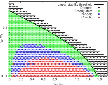
the other⑀-thresholds are the same as above. The character-ization of the behavior of the wave amplitude obtained by the BB-solver is shown in Fig.6. The 391 simulations used for this plot required approximately 15 000 CPU h on an Altix3700Bx2 array of Intel Itanium2 processors.

The agreement between the linear stability threshold and the boundary between linearly stable and unstable simula-tions confirms that the problem of recurrence is taken care of by the free streaming test in the categorization algorithm. When␥dⰆ␥L and ␯aⰆ␥d, a bursty behavior, characterized

by a succession of bursts with characteristic growth and de-cay rates of ␥L and ␥d, respectively, and with a quiescent

phase in between that lasts a time 1/␯a, as described in Ref.

28, is expected. A few solutions in the chaotic region appear to follow this picture. However, most of the chaotic solutions do not feature a significantly quiescent phase. Consequently,

0.01 0.1 0 0.2 0.4 0.6 0.8 1 1.2 1.4 1.6 νa / ω0 γd/ ω0

Linear stability threshold Damped Steady state Periodic Chaotic

FIG. 5. 共Color online兲 Behavior bifurcation diagram. The classification of each solution is plotted in the共␥d,␯a兲 parameter space. The solid curve is

the linear stability threshold obtained by solving the linear dispersion rela-tion numerically. The parameters of these simularela-tions are Nx⫻Nv= 64

an attempt at sorting out a pulsating regime from the chaotic region seems vain. For small collision rates, we observe in-stabilities in the linearly stable region, which suggests the possibility of subcritical instabilities. This effect is not dis-cussed in this article but will be the subject of future work. The physics of several region of this diagram is discussed in the following subsections.

A. Steady state above marginal stability_„␥dÈ␯a™␥L…

In the parameter region where external damping and dis-tribution relaxation are of the same order and both are small compared to the linear drive, we expect and observe the satu-ration of the wave amplitude to a steady state in the time-asymptotic limit. We assume a rate of annihilation of the beam particles much smaller than the saturated bounce fre-quency,␯aⰆ␻b at t→⬁. We also assume that the resonant

region is narrow compared to the resonant velocity, 4␻b/k

Ⰶ␻/k, so that we can assume that the contribution to the resonant power transfer comes from a narrow region around the resonant velocity. Berk and Breizman derived a relation yielding the saturation level in this situation,11

␻b= 1.96

␯a

␥d

␥L. 共24兲

Thus, if we normalize all quantities to the linear growth rate, then within the aforementioned assumptions, the saturation level depends only on the ratio of␯a to␥d.

We investigate the validity of this theory by numerically computing the scaling law for the saturation level at a given normalized relaxation rate␯a/␥L= 0.1. In a previous work,20

such a scan has been done using a reduced model particle code, and the results showed good agreement with the ana-lytic prediction in a region where␥d⬃␯a. Figure7shows the

saturation level obtained from the analytical theory, Eq.共24兲, from reduced model simulations, and from full-f simulations with the BB-solver. When the initial distribution is the one used in Fig.6, we observe quantitative agreement between the theory and both reduced model and full-f simulations in the parameter region␥d⬃␯a.

To reveal the limitations of the reduced model, the same computation is done for a distribution with a slightly in-creased beam density 共nB/n0= 0.15兲 and decreased beam

temperature 共vB/vth= 2.5兲, giving ␥L/␻0= 0.067 instead of

0.032. When we use the reduced model, the scaling law is roughly independent of ␥L and is in agreement with the

theory in the parameter region ␥d⬃␯a, in accordance with

the aforementioned work. On the other hand, when we take into account the evolution of bulk plasma, we observe a sig-nificant dependency of the saturation amplitude on the linear growth rate. For larger␥L, we find some discrepancy from

the analytical prediction in the low ␥d region because the

island width becomes of the order of the resonant velocity 共The island width normalized to the resonant velocity is given by 0.14␻b/␥Lin the low-␥Lcase and by 0.29␻b/␥Lin

the higher-␥Lcase.兲 This result shows that it is necessary to

take into account the effect of bulk particles to accurately discuss the validity limit of the theory.

B. Steady state and periodic solutions near marginal stability_„␥É␥L−␥d™␥L…

When ␥Ⰶ␥L, a reduced integral equation for the time

evolution of the electric field amplitude has been developed using an extension based on the closeness to marginal stability.6Within the assumption␻b/␥Ⰶ1,

10-4 10-3 0.01 0.1 0 0.01 0.02 0.03 0.04 νa /ω 0 γd/ω0

Linear stability threshold Damped Steady state Periodic Chaotic Chirping

FIG. 6. 共Color online兲 Behavior bifurcation diagram for a cold bulk, weak warm beam distribution for which␥L/␻0= 0.0324. The classification of each

solution is plotted in the共␥d,␯a兲 parameter space. The solid curve is the

linear stability threshold obtained by solving the linear dispersion relation numerically. The parameters of these simulations are CFL= 3.0, vmax

= 18vth,vmin= −10vth, Nv= 2048, and Nxranges from 128 to 256. Diamonds

and triangles on the right of the linear stability threshold, which are not included in the legend, represent subcritical instabilities.

0 2 4 6 0 0.1 ωb /γ L γd/γL νa/γL Analytic theory Reduced model (LowγL)

Reduced model (HigherγL)

Full-f (Lowγ_L) Full-f (Higherγ_L)

FIG. 7. 共Color online兲 Saturation level at a given collision frequency

␯a/␥L= 0.1 for both the distribution of Fig.6共Low-␥Lcase兲, and a

distribu-tion with increased beam density共Higher-␥Lcase兲. The numerical

d␻b2 dt =共␥L ⴱ_−␥ d兲␻b 2 −␥L ⴱ 2

冕

t_/2 t dt1

冕

t−t1 t₁ dt2共t − t1兲2 ⫻ e−␯a共2t−t1−t2兲␻ b 2_共t 1兲␻b 2_共t 2兲␻b 2_{共t + t} 2− t1兲, 共25兲

where␥Lⴱ is the linear growth rate obtained by solving

ana-lytically the dispersion relation for ␥d=␯a= 0 in the ␥,

冑

2kvthⰆ␻ limit, ␥Lⴱ⬅ ␲ 2n0 ␻0 2_␻ k2

冏

⳵f0 ⳵v

冏

_v=␻/k. 共26兲

For a cold bulk, warm beam distribution, an analytic treat-ment of the dispersion relation共22兲yields

␥⬇␥Lⴱ−␥d, 共27兲

which agrees with the linear part of the latter integral Eq.

共25兲. In Ref.6, the analytic treatment is carried on by nor-malizing the time by␥Lⴱ−␥d.

We observe that the relation共27兲 is a good approxima-tion in most of the parameter space. However, as we get closer to the linear stability threshold, the relative error 兩␥Lⴱ−␥d−␥兩/共兩␥Lⴱ−␥d兩+兩␥兩兲 approaches unity. In addition, for

our choice of distribution, there is a 14% discrepancy be-tween the value of ␥Lⴱ/␻0= 0.0373 and ␥L/␻0= 0.0324, the

numerical solution of the eigenvalue problem. We infer that we can replace␥Lⴱ−␥dby␥in the integral Eq.共25兲and use␥

itself as the relevant choice of normalization parameter. This procedure yields a steady solution,

␻b2= 2

冑

2␯a2

冑

␥

␥Lⴱ

. 共28兲

A series of simulations near marginal stability 共0.005 ⬍␥/␥L⬍0.02兲, for ␯a spanning two orders of magnitude,

confirms the validity of the latter expression. Figure8shows quantitative agreement with the saturation level of the nu-merical solutions.

Nonlinear stability analysis reveals that the constant so-lution共28兲 is unstable when ␯a⬍␯cr, with ␯cr= 4.4␥. To

as-sess this criterion for the bifurcation from a steady-state so-lution to a periodic soso-lution, a zoom in the behavior bifurcation diagram共Fig.6兲 of the region near marginal

sta-bility where this bifurcation occurs is presented in Fig.9. We observe a qualitative agreement between the steady-periodic boundary and␯cr. However, when␥/␥L⬍0.01, chaotic

solu-tions appear for␯Ⰷ␯cr. This discrepancy is explained by the

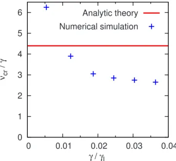
existence of nonlinear excitations. As we approach marginal stability, the nonlinear behavior becomes sensible to the ini-tial perturbation level. To prove this point, we perform a series of simulations in the vicinity of the bifurcation with an initial amplitude reduced from ␻b/␥L= 0.3 to ␻b/␥L

= 3⫻10−7_{. Figure10shows the values of␯/␥ for the}

bifur-0.01

0.1

0.01

0.1

ω

b

/(

8γ

/γ

L

)

1/4

ν

_a

/ ω

₀

Analytic theory

Numerical result

FIG. 8.共Color online兲 Saturation level of solutions near marginal stability for the distribution and the numerical parameters of Fig.6.

0.002 0.003 0.005 0.008 0.034 0.035 0.036 0.037 0.038 νa / ω0 γ_d/ ω0

Linear stability threshold Damped Steady state Periodic Chaotic ν = νcr

FIG. 9.共Color online兲 Zoom in the behavior bifurcation diagram 共Fig.6兲 of

the region near marginal stability where the steady state periodic bifurcation occurs, along with the critical distribution relaxation. Diamonds on the right of the linear stability threshold, which are not included in the legend, cor-respond to subcritical instabilities.

0

1

2

3

4

5

6

0

0.01

0.02

0.03

0.04

ν

cr

/γ

γ / γ

_L

Analytic theory

Numerical simulation

FIG. 10.共Color online兲 Critical distribution relaxation for steady state pe-riodic bifurcation near marginal stability.

cation between steady-state and periodic solutions. We con-firm that␯cr/␥ stays close to the predicted value of 4.4 for

smaller values of␥.

C. Frequency sweeping_„␯a<␥™␥L…

In the collisionless limit, the integral Eq.共25兲is consis-tent with explosive solutions that diverge in a finite time, which suggests that the mode energy is partitioned into sev-eral spectral components. The resulting sideband frequencies have been observed to shift both upwardly and downwardly,4 the frequency shift␦␻共t兲 increasing in time, until the corre-sponding resonant velocities reach lower velocity gradient regions. Reference8shows how we can isolate one spectral component and model it by a BGK wave to obtain the time evolution of one chirping event. In the regime where␦¨␻/␻b3,

␻˙b/␻b2, and ␻b/␦␻Ⰶ1, frequency sweeping is obtained as

␦␻共t兲 ␥Lⴱ = 16 3␲2

冑

2 3␥dt, 共29兲

and a steady-state solution is given by

␻b/␥Lⴱ= 16/3␲2. 共30兲

When␥d is finite and ␯a is small enough, we observe such

chirping solutions in our simulations. Figure 11 shows the time evolution of the field amplitude, when␥d= 0.938␥Lⴱand

␯a= 2.7⫻10−3␥Lⴱ, so that ␥= 0.05␥Lⴱ. The simulation result

agrees with a numerical solution of the reduced Eq. 共25兲, until the field amplitude exceeds the applicability limit. After saturation, the solution is close to the analytic prediction Eq.

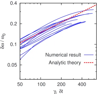
共30兲. Figure 12 shows the time evolution of the wave fre-quency power spectrum obtained with a moving Fourier win-dow. Frequency sweeping events occur repetitively as the slope of the distribution is successively recovered and flat-tened. The time evolution of each chirping is slightly vari-able. To quantify the agreement with theory, we extract the 12 largest upshifting branches. In Fig. 13, we show these branches shifted to the same initial conditions, where each point is obtained by interpolating local maxima from the discrete frequency spectrum. From this plot, we conclude that before border effects occur, chirping evolution follows a square-root law in time, as expected from theory. This sug-gests a possibility to recover the product ␥Lⴱ

冑

␥d from such

power spectrum. By fitting a square-root law to the branches

of Fig. 13, we obtain an average value of ␥_Lⴱ

冑

␥d= 0.0057,

with a standard deviation of 14%, when the input value is

␥Lⴱ

冑

␥d= 0.0061. When a plasma is close to marginal stability

as in the experiment, we can assume␥_Lⴱ⬃␥d共␥Lⴱ

冑

␥d⬃␥d3/2兲,

and this chirping diagnostics may be used to estimate the extrinsic damping rate of the bulk plasma␥d. The agreement

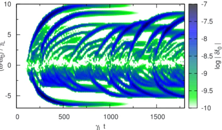
of the expression Eq.共29兲with chirping found in experimen-tal devices29 supports this claim. As we consider a single mode with a fixed wave number, a frequency sweeping cor-responds to the evolution of some structures in the velocity distribution. In Fig. 14, we observe formation of hole and clump pairs in phase space, and they show clear correlation with peaks of the power spectrum shown in Fig.12. It should be noted that near marginal stability,␥d⬎0.4␥Lis given as a

necessary condition for hole-clump pair creation.4 There is yet no theory in the opposite limit␥⬃␥L, and in our

simu-lations we observe frequency sweeping even when␥dⰆ␥L.

0 1 0 50 100 ωb / γL γ_Lt 16 3π2 Simulation Reduced equation

FIG. 11. 共Color online兲 Time evolution of the normalized field amplitude, obtained from full-f simulation and from the reduced Eq.共25兲. In this simu-lation, the initial amplitude has been reduced to␻b/␥L= 0.1 to emphasize the

behavior before saturation.

0 500 1000 1500 γLt -5 0 5 10 (ω -ω0 )/ γL -5 -4 -3 -2 -1 0 lo g|S ω /S0 |

FIG. 12.共Color online兲 Logarithmic scale plot of the time evolution of the frequency power spectrum for␥d= 0.938␥Lⴱ,␯a= 2.7⫻10−3␥Lⴱ. At each time,

the spectrum is normalized to its maximum value.

0.05

0.2

0.4

0.1

50

100

200

400

δω

/ω

0

γ

_L

δt

Numerical result

Analytic theory

FIG. 13.共Color online兲 Time evolution of the 12 largest upshifting branches in logarithmic scale. The dashed curve is the analytic prediction Eq.共29兲.

The Fourier spectrum is shown in Fig. 15 for ␥d/␥L= 0.2,

␯a/␥L= 0.02. Although the chirping is not as pronounced as

in Fig.12, we observe that the dominant frequency sweeps 5% of its initial value.

V. CONCLUSION

In this work, we presented a full-f Vlasov code to solve the BB model for a bump-on-tail distribution. The code was verified by checking its convergence and conservation prop-erties, benchmarked against numerical simulations in former works, and validated against well-known linear and nonlin-ear theories.

We chose the plasma parameters so that we could ex-plore the theory in several parameter regimes with the same initial distribution function. Since the theory considers the interaction between the wave and resonant particles only, we designed the collision operator so that collisions acted only on the beam particles. The feasibility of long-time simula-tions for a low-␥Ldistribution hinged upon the quick

conver-gence and strong stability properties of the CIP-CSL scheme. We performed a scan of the fully nonlinear evolution of the electric field in the whole 共␥d,␯a兲 parameter space. A new

diagnostics allowed us to identify the chirping region. Al-though holes and clumps were not expected to appear when

␥d⬍0.4␥L, we found that the frequency sweeping region can

expand to a low external dissipation regime, around ␥d

⬇0.2␥L. Also, nonlinearly unstable solutions in the linearly

stable region have been detected. Numerical results show a good quantitative agreement with theory in several regimes.

The limits of validity correspond to the assumptions used in deriving the theory. A perturbative numerical approach which does not take into account the kinetic response of the bulk may feature spurious agreement outside of the validity limits when the resonant region reaches a non-negligible portion of bulk particles. We showed how one can identify␥d by

ana-lyzing the time evolution of frequency shifting.

In future works, we will take a detailed look at the mechanism behind hole-clump pairs creation, and consider the dependency of chirping velocity to the time dependent slope of the distribution at the onset. We may also apply the theory of frequency sweeping to tokamak experiments. Moreover, subcritical instabilities will be investigated. It is important to understand the mechanism of such instabilities in the linearly stable region as an experimental device must take a path that go through this region as chirping emerges.

ACKNOWLEDGMENTS

This work was performed within the frame of a co-thesis agreement between the doctoral school of the Ecole Poly-technique, the Japan Atomic Energy Agency, and the Com-missariat à l’Energie Atomique. It was supported by both the JAEA Foreign Researcher Inviting Program and the Euro-pean Communities under the contract of Association between EURATOM and CEA. The views and opinions expressed herein do not necessarily reflect those of the European Commission.

APPENDIX A: THE CIP-CSL SCHEME To solve the general 1D advection equation,

⳵tF + u⳵_␭F = 0, 共A1兲

in a conservative form, we evolve both F and its integrated value R. F˜n共R˜n兲 is the continuous interpolated solution for F共R兲 at the time tn= n⌬t. Fm

n

is the discrete value of F˜n_{at the}

grid point of coordinate␭m= m⌬␭ and

Rm n =

冕

␭m ␭m+1 F ˜n_{共␭兲d␭. 共A2兲}

Fn_{is an array which contains the values F} m n

for every point m on a grid point of coordinate␭m. We define the 1D algorithm

CIPCSL1D共u,Fn_{, F}n+1_{, R}n_{, R}n+1_{,␭,⌬␭,⌬t兲 as follows.}

For each m, • define␭p_m⬅␭m− u⌬t.

• Find the grid point kmsatisfying␭k_mⱕ␭p_mⱕ␭k_m+1 and

de-fine 具␭m典⬅␭p_m−␭k_m.

• Define the coefficients

␾k_m⬅ Fk_m n + Fk_m+1 n ⌬␭2 − 2Rk_m n ⌬␭3, 共A3兲 ␩k_m⬅ − 2Fk_m n + Fk_m+1 n ⌬␭ + 3Rk_m n ⌬␭2. 共A4兲 • Advect R, 0 500 1000 1500 γ_Lt -5 0 5 10 (ω -ω0 )/ γL -10 -9.5 -9 -8.5 -8 -7.5 -7 log |δ f0 |

FIG. 14. 共Color online兲 Logarithmic scale plot of the time evolution of

␦f0⬅ f¯− f0, normalized to n0/vth, for␥d= 0.938␥Lⴱ,␯a= 2.7⫻10−3␥Lⴱ. 750 800 850 900 950 γLt -2 -1 0 1 2 (ω -ω0 )/ γL -5 -4 -3 -2 -1 0 lo g|S ω /S 0 |

FIG. 15.共Color online兲 Logarithmic scale plot of the time evolution of the frequency power spectrum for␥d= 0.2␥L,␯a= 0.02␥L.

Rm n+1 = Rk_m n + D_m+1n − Dm n , 共A5兲 where Dm n =␾k_m具␭m典3+␩k_m具␭m典2+ Fm n_具␭ m典. 共A6兲 • Advect F, Fm n+1 = 3␾k_m具␭m典2+ 2␩k_m具␭m典 + Fm n . 共A7兲

This 1D algorithm is extended to the 2D phase space 共x,v兲 in the following way. fi,j

n

is the value of the distribution f at the grid point of coordinates xi= i⌬x, vj=vmin+ j⌬v at the

time tn= n⌬t. We define the density within a cell and the line

densities, ␳i,j n =

冕

x_i x_i+1

冕

vj vj+1 f˜n共x,v兲dxdv, 共A8兲 ␴xi,j n =

冕

x_i x_i+1 f˜n共x,vj兲dx, 共A9兲 ␴vi,j n =

冕

vj vj+1 f˜n共xi,v兲dv. 共A10兲

The first advection in the x-direction is performed by calling successively, for each j,

CIPCSL1D共v¯j,␴v n ,␴_vⴱ,␳n,␳ⴱ,x,⌬x,⌬t/2兲, CIPCSL1D共vj, fn, fⴱ,␴x n ,␴xⴱ,x,⌬x,⌬t/2兲,

with v¯j⬅共vj+vj+1兲/2. Similarly, the advection in the

v-direction is performed by calling successively, for each i, CIPCSL1D共qE¯i/m,␴xⴱ,␴xⴱⴱ,␳ⴱ,␳ⴱⴱ,v,⌬v,⌬t兲,

CIPCSL1D共qEi/m, fⴱ, fⴱⴱ,␴vⴱ,␴vⴱⴱ,v,⌬v,⌬t兲,

with E¯i⬅共Ei+ Ei+1兲/2. Then we repeat the advection in the

x-direction,

CIPCSL1D共v¯j,␴vⴱⴱ,␴v n+1

,␳ⴱⴱ,␳n+1,x,⌬x,⌬t/2兲, CIPCSL1D共vj, fⴱⴱ, fn+1,␴xⴱⴱ,␴xn+1,x,⌬x,⌬t/2兲.

Here, the subscriptsⴱ and ⴱⴱ were used to designate inter-mediate steps between tnand tn+1. To avoid spurious leakage

of particles, we impose a zero flux at the velocity boundaries by setting

具␭j=1典 = 具␭j=N_v典 = 0. 共A11兲

APPENDIX B: TIME-SERIES CATEGORIZATION ALGORITHM

The algorithm we developed to categorize the behavior of each numerical solution is an improved version of the algorithm designed by Vann,7 with an other way of sorting out chaotic from periodic behavior, a new diagnostics to dis-tinguish chirping from merely chaotic solutions, and where we take into account numerical issues, which appear when

␥Lis smaller.

The categorization is based on an analysis of the time series of the normalized electric field energy, A共t兲⬅E共t兲/E0,

withE0= n0mvth2/2. First, we define the global minimum as

Agm⬅min兵A共t兲其0⬍t⬍tmax, where tmax is the time duration of the simulation. Then we drop the initial transient phase and extract a time window tmin⬍t⬍tmax over which A共t兲 is

sampled at a rate⌬ts. Here, tminis an estimation of the time

duration of the transient phase. Within this window, we de-fine the mean value 具A典, maximum Amax⬅max兵A共t兲其 and

minimum Amin⬅min兵A共t兲其, the oscillation amplitude ⌬A

⬅Amax− Amin, and the local minima 共maxima兲 as points

where A共t兲 is smaller 共larger兲 than A共t−⌬ts兲 and A共t+⌬ts兲.

As a measure of the periodicity, we compute the two point correlation function as R共␶兲 = 1 m

兺

_j=0 m−1 具A˜j共␶,␶

⬘

兲A˜j+1共␶,␶

⬘

兲典

冑

具A˜j共␶,␶

⬘

兲2典

冑

具A˜j+1共␶,␶

⬘

兲2典 , 共B1兲

where for each correlation window size␶, A

˜

j共␶,␶

⬘

兲 ⬅ A共tmax− j␶−␶

⬘

兲 − 具A共tmax− j␶兲典. 共B2兲

m =共tmax− tmin兲/␶is the number of period included inside the

total time window and the angular brackets represent the time-average over a period,

具A˜共␶,␶

⬘

兲典 =1

␶

冕

0

␶

A

˜ 共␶,␶

⬘

兲d␶

⬘

. 共B3兲 The overall correlation R0is defined as the maximum of R共␶兲

for ␶⬎␶c, where ␶c is the shortest period such that R共␶c兲

ⱕ0. In other words, R0 is the normalized amplitude of the

peak in the two point correlation function corresponding to the dominant frequency. This measure which is used to sort out chaotic from periodic behavior is different from the one given in Ref.7. We also provide a criterion to sort out chirp-ing solutions. We compute the frequency power spectrum of the time evolution of the electric field at some position, E共x=0,t兲, and normalize the amplitude of the spectrum to its maximum value. At each time, we extract the largest and smallest frequency for which the amplitude in the power spectrum is significant, i.e., larger than a threshold⑀6. Then,

we define ⌬␻max as the maximum difference between the

largest and smallest frequency, normalized to the plasma fre-quency. We then proceed to the following decision tree: 共1兲 if Agm⬍⑀0, then damped.

共2兲 Else if ⌬␻max⬎⑀7, then chirping.

共3兲 Else if 具A典⬍⑀1, then damped.

共4兲 Else if A共t兲 is monotonic and ⌬A/具A典⬍⑀2, then

steady-state.

共5兲 Else if A共t兲 is monotonically decreasing 共zero local ex-trema兲, then damped.

共6兲 Else if each minima 共maxima兲 is larger 共smaller兲 than the former or⌬A/具A典⬍⑀3or⌬A⬍⑀4, then steady-state.

共7兲 Else if R0⬎1−⑀5, then periodic.

共8兲 Else if the number of extrema is not less than four then chaotic,

Spe-cial care is taken in adjusting ⑀7 empirically so that

fre-quency splitting is not mistaken for frefre-quency sweeping. In this decision tree, the logical test B3 is an addition to the one given in Ref.7. For damped solutions, as the electric field becomes small, the particles experience free streaming, leading to spurious recurrence effects after half the recur-rence time TR/2=␲/k⌬v. Free streaming occurs when

兩qE0兩TR/m⬍⌬v, and ⑀0 is chosen to reflect this condition.

For the benchmark, this logical step is switched off as the recurrence effect is less problematic for shorter-time simula-tions.

1_{H. V. Wong and H. L. Berk,Phys. Plasmas 5, 2781共1998兲.}

2_{X. Garbet, G. Dif-Pradalier, C. Nguyen, P. Angelino, Y. Sarazin, V.}

Grand-girard, P. Ghendrih, and A. Samain,AIP Conf. Proc. 1069, 271共2008兲.

3_{H. L. Berk, B. N. Breizman, and M. S. Pekker, Plasma Phys. Rep. 23, 778}

共1997兲.

4_{B. N. Breizman, H. L. Berk, M. S. Pekker, F. Porcelli, G. V. Stupakov, and}

K. L. Wong,Phys. Plasmas 4, 1559共1997兲.

5_{A. Fasoli, B. N. Breizman, D. Borba, R. F. Heeter, M. S. Pekker, and S. E.}

Sharapov,Phys. Rev. Lett. 81, 5564共1998兲.

6_{H. L. Berk, B. N. Breizman, and M. Pekker,Phys. Rev. Lett. 76, 1256}

共1996兲.

7_{R. G. L. Vann, R. O. Dendy, G. Rowlands, T. D. Arber, and N.}

d’Ambrumenil,Phys. Plasmas 10, 623共2003兲.

8_{H. L. Berk, B. N. Breizman, and N. V. Petviashvili,Phys. Lett. A234, 213}

共1997兲.

9_{H. L. Berk, B. N. Breizman, and N. V. Petviashvili,Phys. Lett. A238, 408}

共1998兲.

10_{H. L. Berk, B. N. Breizman, J. Candy, M. Pekker, and N. V. Petviashvili,}

Phys. Plasmas 6, 3102共1999兲.

11_{H. L. Berk and B. N. Breizman,Phys. Fluids B 2, 2246共1990兲.} 12_{T. Nakamura, R. Tanaka, T. Yabe, and K. Takizawa,J. Comput. Phys.}

174, 171共2001兲.

13_{I. B. Bernstein, J. M. Greene, and M. D. Kruskal,Phys. Rev. 108, 546}

共1957兲.

14_{B. Breizman, H. Berk, and H. Ye,Phys. Fluids B 5, 3217共1993兲.} 15_{P. Bhatnagar, E. Gross, and M. Krook,Phys. Rev. 94, 511共1954兲.} 16_{M. Lesur, Y. Idomura, and S. Tokuda, JAEA-Research 2006–089, 1, 2007.} 17_{T. Nakamura and T. Yabe,Comput. Phys. Commun. 120, 122共1999兲.} 18_{C. Cheng and G. Knorr,J. Comput. Phys. 22, 330共1976兲.}

19_{G. Strang,SIAM共Soc. Ind. Appl. Math.兲 J. Numer. Anal. 5, 506共1968兲.} 20_{H. L. Berk, B. N. Breizman, and M. Pekker,Phys. Plasmas 2, 3007}

共1995兲.

21_{J. R. Cary and I. Doxas,J. Comput. Phys. 107, 98共1993兲.} 22_{L. Landau, J. Phys.共Paris兲 10, 25 共1946兲.}

23_{B. Davies,J. Comput. Phys. 66, 36共1986兲.}

24_{B. D. Fried, C. S. Liu, R. W. Means, and R. Z. Sagdeev, National}

Tech-nical Information Service Document No. AD730123 PGG-93, University of California, Los Angeles共1971兲. Copies may be ordered from the Na-tional Technical Information Service, Springfield, Virginia 22161.

25_{E. Fijalkow,Comput. Phys. Commun. 116, 319共1999兲.}

26_{F. Xiao, T. Yabe, G. Nizam, and T. Ito,Comput. Phys. Commun.94, 103}

共1996兲.

27_{F. Xiao, T. Yabe, X. Peng, and H. Kobayashi,J. Geophys. Res.,关Atmos.兴}

107, 4609, doi:10.1029/2001JD001532共2002兲.

28_{H. L. Berk, B. N. Breizman, and H. Ye,Phys. Rev. Lett.68, 3563共1992兲.} 29_{S. D. Pinches, H. L. Berk, D. N. Borba, B. N. Breizman, S. Briguglio, A.}

Fasoli, G. Fogaccia, M. P. Gryaznevich, V. Kiptily, M. J. Mantsinen et al.,