Climatic changes in temperature and salinity in the subtropical North Atlantic

(1)

CLIMATIC CHANGES IN TEMPERATURE AND

SALINITY IN THE SUBTROPICAL NORTH ATLANTIC

by

Alicia Maria Lavin Montero

Licenciada en Ciencias Fisicas Universidad de Cantabria (Spain)

(1977)

Submitted to the Department of Earth, Atmospheric and Planetary Science in partial fulfillment of the

requirements for the degree of Master of Science in Physical Oceanography

at the

MASSACHUSETTS INSTITUTE OF TECHNOLOGY May 1993

@ Alicia M. Lavin Montero 1993

The author hereby grants to MIT permission to reproduce and to distribute copies of this thesis document in whole or in part.

Signature of Author ... ... ... - " "en Earth, Atmospheric and Planetary Science A Massachusetts Institute of Technology May 19, 1993

Certified by... ...

Carl Wunsch

/{ecil

and Ida Green Professor of Physical Oceanography Thesis Supervisor

Accepted by ... .. ... ... .. ... .... - . Thomas H. Jordan

Department Head,

W

ITHI

N

Institute of Technology

MIT

-ENSTIT

(2)

(3)

CLIMATIC CHANGES IN TEMPERATURE AND SALINITY IN THE SUBTROPICAL NORTH ATLANTIC

by

Alicia Maria Lavin Montero

Submitted in partial fulfillment of the requirements for the degree of Master of Science in Physical Oceanography at the

Massachusetts Institute of Technology May 19, 1993

Abstract

Three sets of hydrographic data are used to examine the changes in tem-perature and salinity in the subtropical North Atlantic. Transatlantic hydrographic sections at 24.50N were obtained in October 1957, in August 1981, and finally in July-August 1992.

A general warming was found over the upper 3000 m of the North Atlantic at 24.50N, over the entire 35-year period. There is high variability over time over most of the upper 1000 m. In the layer between 1000 m and 3000 m, a significant warming of 0.1±0.02 'C has been observed. The rate of warming is 0.030C/decade and is nearly steady in the two periods. Significant cooling is found in water deeper than 3000 m in both the North American (-0.027±0.016 oC) and the Canary Basins (-0.013±0.005 oC). There are some indications that the

/S

relationship at 24.5 ON has changed over time. The nonuniform change of the depth of isotherms, due to the diverse pattern of warming or cooling, results in a change in the volume of water masses. Expansion in the North American Basin occurs in the transition zone between Antarctic Bottom Water and lower North Atlantic Deep Water, with a rate of 9 km2/year. In the Canary Basin the expansion is larger and has mostly taken place in the last 11 years. Contraction occurs in the North Atlantic Deep Water, and expansion in the thermocline water.

Finally, using a simple heat calculation, we find that there is no significant difference between the heat flux estimated from the three surveys performed in 1957, 1981, and 1992 at 24.50N .

Thesis Supervisor: Carl Wunsch,

Cecil and Ida Green Professor of Physical Oceanography Department of Earth, Atmospheric and Planetary Sciences Massachusetts Institute of Technology

(4)

Acknowledgments

I would first like to thank my thesis advisor, Carl Wunsch, for his guidance and patience during the research. To Harry Bryden for his continuous support and advice during the cruise and after it, he was always ready to help me. To Bob Millard, he had to work hard to finish the cruise calibrations on time to be used for the thesis, and he generously spared his time for me. To T. Joyce and M. McCartney for their helpful comments about the results. To Charmaine King for her assistance in data and computer matters. To Alison MacDonald, Gwyneth Hutfford, Jim Gunson and many others fellow students and post-docs that have help me with the thesis and the subjects.

To Rafael Robles, Director, and Alvaro Fernandez, Subdirector of the Instituto Espafiol de Oceanograffa (IEO), Ministerio de Agricultura, Pesca y Alimentaci6n, my employer, Orestes Cendrero, Director of Centro Oceanogrifico de Santander (IEO), F. F. Castillejo and J.R. Pascual for allowing me to come to MIT and supporting me during this period of study.

To Gregorio Parrilla (IEO), chief scientist of the Hesperides cruise, and all the participants of the cruise. Gregorio gave me complete freedom to work the data, and worked hard, with M. Jesus Garcia in the final calibration of the cruise data.

To Miguel Losada, Professor of Ocean Engineering, University of Cantabria. To the Fundaci6n Marcelino Botfn (Santander, Spain) that funded me to stay at MIT, without it I couldn't have obtained this Master Degree.

To my husband Mac for his support in many difficult moments during this period and his Fulbright grant that allowed us to spend this time of study at M.I.T. This research was mainly supported by the Fundaci6n Marcelino Botifn (San-tander, Spain), the Instituto Espafiol de Oceanograffa, NSF OCE-9114465 and NSF OCE-9205942 also contributed

(5)

Introduction

As scientific understanding of the causal mechanisms for environmental changes im-proves there is an accompanying public awareness of the susceptibility of the present environment to significant regional and global change. Understanding the basic mech-anisms of climate is a key to early detection of change in the earth's climate system.

Since the ocean-atmosphere system is driven by the sun's radiation, it is im-portant to know what the response of the system is to the known radiative input. The ocean carries a significant fraction of the meridional heat flux that makes the middle latitudes of the earth habitable. Vonder Haar and Oort (1973) found that in the region of maximum net northward energy transport by the ocean-atmosphere system (30-350N) the ocean transports 47% of the required energy. At 200_{N, where the ocean} transport reaches a maximum, they estimate that the ocean accounts for 74% of the total meridional heat transport. So the ocean is critical in the redistribution of solar energy.

The Atlantic Ocean is the most saline of all the world oceans. It has significant exchange of water masses, heat and salt with several marginal seas, regions in which important transformations of water masses take place. A complex thermohaline-driven circulation moves water masses both northward and southward along its west-ern boundary regions. The Atlantic Ocean has been well surveyed in the twenti-eth century with various large scale surveys such as International Geophysical Year (IGY), Geochemical Ocean Sections Studies (GEOSECS), Long Lines (LL), South

(8)

Atlantic Ventilation Experiment (SAVE) and the World Ocean Circulation Experi-ment (WOCE). The Atlantic is the source of North Atlantic Deep Water (NADW), and in it can be found several other important water masses: Mediterranean Water, Antarctic Intermediate Water (AAIW) and Antarctic Bottom Water (AABW).

The 24.50N transatlantic section is an archetypic transoceanic hydrographic section. It is rich in water masses and crosses the North Atlantic in the middle of the subtropical gyre. It provides a census of major intermediate, deep and bottom water masses whose sources are in the Antarctic and far northern Atlantic as well as estimates of the thermohaline circulation of these water masses and of the wind-driven circulation in the upper water column. Furthermore, the 24.50N section crosses the northward flowing Gulf Stream through the Florida Straits and the southward wind-driven Sverdrup flow in mid-ocean at essentially the latitude of maximum wind stress curl.

The 24.50N section was measured in 1957 (IGY data) (Fuglister, 1960), and 1981 (Roemmich and Wunsch, 1984). Although hydrography is a traditional method for obtaining the geostrophic flow throughout the water column, the quantity and quality of the measurements have been dramatically increased since the use of elec-tronic instrumentation such as CTD (Brown, 1974). This new technique has been used in the later periods of sampling.

From analyses of the 1957 section, Hall and Bryden (1982) determined that the Antarctic Intermediate water flows northward across 240N between 600 and 1100 m depth, North Atlantic deep water flows southward between 1200 and 4500 m, and Antarctic bottom water flows northward below 4500 m depth. They found a vertical meridional cell with a net northward flow across 240N of 18 x 106 m3/s of warmer water in the upper 1000 m of the water column and a southward return as intermediate and deep water between 1000 and 4500 m depths. Roemmich and Wunsch (1985) reported a similar pattern of water masses and meridional flow on the 1981 section.

(9)

The 24.50N section was one of the sections repeated during WOCE (section A-5, WOCE Implementation Plan) which Gregorio Parrilla from the Instituto Espaiiol de Oceanograffa (IEO), proposed to the Spanish government. For this proposal, Par-rilla had the important support of Harry Bryden and Robert Millard from Woods Hole Oceanographic Institution. Parrilla obtained the approval of his proposal with the help of two favorable conditions. First in 1992 Spain was celebrating the Quincen-tennial of one important episode in its modern history The Discovery of America. In 1492 Columbus and his Spanish sailors left Palos de Moguer (Golfo de Cadiz) for the Islas Canarias. After that, they sailed westward approximately at 24°N reaching San Salvador (Bahamas Islands) on October 12, 1492. The second favorable circumstance was the building of a new oceanographic ship for the Spanish Antarctic Program.

The cruise was carried out in July-August of 1992 with the participation of scientists from the Instituto Espaiiol de Oceanograffa, Woods Hole Oceanographic Institution, and other Spanish and American institutions such as Instituto de In-vestigaciones Marinas, Centro de Estudios Avanzados de Blanes, Ciencias del Mar de la Universidad de Las Palmas, Universidad de La Corufia, Programa de Clima Maritimo del MOPT, Ainco-Inter Ocean, Lamont Doherty Geological Observatory, and RSMAS University of Miami.

The objective of this research is to quantify the response of the ocean to the warmer atmospheric conditions of the last decade and compare the conditions with previous surveys. Roemmich and Wunsch (1984) reported warming between 700 and 3000 m, and weak cooling above and below those depths. We have done the same calculation for the two periods of comparison 1957-1981 and 1981-1992. The procedure was as follows. First, the comparison was made using two methods based on cubic splines and objective mapping, and the differences between the cruises and the zonal average of the differences were calculated. Next, the area occupied by the different water masses in the three cruises was calculated, and these areas are related

(10)

to the strength of their possible sources. The changes in the temperature/salinity relationship are examined.

Second, we discuss the transport of heat. Using a simple heat calculation, we have tried to see whether the heat transport across 240N has changed in time from one cruise to other.

(11)

Chapter 1 Description of the Data

1.1 Introduction

The objective of this research is to investigate the climatic variations of temper-ature, salinity, and heat fluxes over the subtropical Atlantic Ocean from the surface to 6000 m depth during the last 35 years. The data used includes three oceano-graphic cruises on which zonal hydrooceano-graphic sections at latitude 24.50N were carried out: the first one in October 1957, by the British R.R.S. Discovery II of the National Institute of Oceanography (Chief Scientist L.V. Worthington, Woods Hole Oceano-graphic Institution) during the International Geophysical Year (Fuglister 1960); the second one in August 1981, by the R.V. Atlantis Ilof the Woods Hole Oceanographic Institution (Chief Scientist D. Roemmich, at that time Woods Hole Oceanographic Institution) (Roemmich and Wunsch, 1985); the last one in July-August of 1992 by the Spanish B.I.O. Hespirides of the Armada Espaiiola, (Chief Scientist Gregorio

Parrilla, Instituto Espafiol de Oceanograffa).

The section chosen is situated in the central part of the subtropical gyre. The transect was done always downwind, westward from Africa to America. It began at the African continental shelf, which is quite flat, with depths increase slowly, reaching

(12)

4000 m around 20°W, and 5500 m around 250W. The bottom of the Canary Basin is situated between 30°and 350_{W, west of this longitude the beginning of the} Mid-Atlantic Ridge becomes apparent. The Mid-Mid-Atlantic Ridge extends until 530W, is centered at about 45°W, with the shallowest parts reaching 3000 m. West of the ridge, the bottom is smooth in the North American Basin with depths between 5500 and 6500 m. The western boundary is quite steep from 5000 m to the Bermuda Bank. The extent of both basins is 3000 Km, but the North American basin is deeper on average than the African basin.

All the data are interpolated to a common set of depths. These depths are closely spaced in the upper waters, with increasing separation toward the bottom. The spacings are chosen to resolve the large structures of the general circulation and the mesoscale variability. Table 1.1 lists the standard depths. Data and interpolation procedures are described here for each cruise.

1.2 Discovery II 1957 IGY Data

There is a detailed description of the cruise in Fuglister (1960). The cruise was carried out between October 6 and October 28, 1957, from 16020'W to 75028'W. The total number of stations was 38 and the sampling was done using reversing thermometers and Nansen bottles.

Temperatures are stated to be accurate within ± 0.01"C, depth is accurate within ± 5 m based on reading of paired protected and unprotected thermometers and salinity is accurate to ± 0.005 /,,o.

Data were converted from depth to pressure using Saunders's formula (Saun-ders, 1981). Temperatures were based on IPTS-48 (International Practical Temper-ature Scale 1948), conversion to IPTS-68 (Barber 1969) is possible by Fofonoff and

(13)

interval 50 1 2 3 4 5 6 7 8 9 10 11 12 13 14 15 16 17 18 19 20 21 22 23 24 25 26 27 28 29 30 31 32 33 34 35 depth 0 50 100 150 200 250 300 400 500 600 700 800 900 1000 1100 1200 1300 1400 1500 1750 2000 2250 2500 2750 3000 3250 3500 3750 4000 4250 4500 4750 5000 5500 6000 500

Table 1.1: Standard depths 100

(14)

Bryden (1975) formula. Differences, however are less than 0.01 in surface and less than 0.002 for temperature lower than 4 OC. Such differences are lower than the ac-curacy of the measurements and therefore the 48 scale were used. Salinities were based on the old scale (part per thousand), before the Practical Salinity Scale, the differences between the two scales are well below the accuracy of the measurements. Therefore, all salinity data used in this research are based in PSS-78 (pss).

For the discrete bottle data, vertical linear interpolation was made between adjacent data points for each station to the standard depths. Data were plotted to check the values and detect errors in interpolation.

1.3 Atlantis II 1981 Long Lines Data

Detailed description of the cruise is in Roemmich and Wunsch (1985). The cruise began August 11 from Las Islas Canarias with the first station off Cape Juby (Morocco). The last station was east of the Bahamas Bank on September 4. Two sections were made across the Florida Current at 26002' N and 27023'N to finish on September 6. The mid-Atlantic section was composed of 90 stations sampled by Neil Brown Instrument CTD/0 2. A 24-bottle rosette water sample was used for CTD-0 2 calibrations (Millard, 1982).

Simple averages of nearly continuous CTD/0 2 measurements are made to de-rive the standard depths values. The 'window' was set 20 m above and 20 m below the standard depths. When the CTD did not reach the bottom to enable interpolation to all available standard depths, linear vertical extrapolation was allowed to estimate one more standard depth from the last two interpolated depths.

(15)

1.4 Hesperides 1992 WOCE Data

The 1992 24.50N section, designated A-5 by WOCE (WOCE Implementation plan), was made by the Spanish B.I.O. Hesperides of the Armada Espaiiola, (Chief Scientist Gregorio Parrilla, Instituto Espafiol de Oceanograffa). The boat departed from C diz on July, 14 sailing to Las Islas Canarias; six stations were made in this track for testing CTDs and rosette.

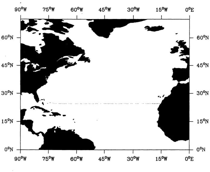
We left Las Palmas on July 20 arriving at station number one (240_29.97'N, 150_{58.08'W) the same day. The section was finished at the Bahamas (24}0_30'N 750_{31'W) after 101 stations on August 14. On August 15, a section of 11 stations} across of the Florida Current at 2603'N was done. Figure 1.1 gives the location of the stations.

Two NBIS/EG&G Mark IIIb CTD underwater units each equipped with pres-sure, temperature, conductivity and polographic oxygen sensors were used throughout the cruise. Their serial number are 1100 and 2326. A General Oceanics rosette fit-ted with 24 Niskin bottles of 10 or 12 liter of capacity was used with the CTD for collecting water samples. In all cases, data were collected from the ocean surface to within a few meters of the bottom.

Both NBIS/EG&G Mark IIIb CTDs were equipped with titanium pressure sensors manufactured by Paine Instrument. The temperature sensor was a Rose-mount platinum # 171. The conductivity sensor is a 3-cm alumina cell manufactured by NBIS/ED&G. The CTD work was supervised by G. Parrilla (IEO) and H. Bry-den (WHOI), software and calibrations by R. Millard (WHOI) and hardware by J. Molinero (IEO) and G. Bond (WHOI).

Water sampling included measurements of salinity, oxygen, nutrients (sili-cate, nitrate, nitrite and phosphate), chlorofluorocarbons (CFC), pH, alkalinity, C0 2,

(16)

60oW 450W 30W 60N 600N 450N - 450N 30ON 300N 150N - 150N OON OON 90W 750W 60aW 450W 30W 150W OOE

Figure 1.1: Section at 24.50N in the North Atlantic. Dots denote the location of stations in the 1992 Hespirides cruise. IGY 1957 track was similar, but spacing between stations was larger than in the 1992 section. Atlantis 1981 was also at that latitude west of 24.5*W. For the comparison I have used this common part.

(17)

particulate matter, chlorophyll pigments, 14C and aluminum. Underway Acoustic Doppler Current Profiler (ACDP) measurements were also taken. Typically, 24 sam-ples were obtained for each station. The water sample salinities were measured with a Guildline Autosal model 8400A salinometer by R. Molina (IEO). Oxygen determi-nations were carried out primarily by J. Escanez (IEO). (G. Parrilla, Cruise report in preparation).

Since in this research we have used only CTD/0 2 data, I will describe only these observations. Data acquisition and calibrations were done following the proce-dures given by Millard and Yang (1993). The EG&G data logging program CTDACQ was used to record down and up profiles and CTDPOST was used to flag spurious data. The remainder of the CTD post-processing was performed using the WHOI PC based CTD processing system as described by Millard and Yang (1993).

The CTD/0 2 profiles require accurate calibration of conductivity, tempera-ture, and pressure sensors in the laboratory. This is particularly important in deep water (below 1500 m) where variations in temperature and salinity are small. CTD pressure, temperature, and conductivity sensors for both CTDs were calibrated at WHOI before and after the cruise. The best fit NBIS/EG&G Mark IIIb CTD sensor calibration is usually found to be linear in conductivity, quadratic in temperature, and quadratic for the titanium pressure transducer (Millard et al., 1993). The poly-nomial coefficients to calibrate the raw sensor data are determined using standard least squares techniques.

Temperature calibrations are based on the International Practical Temperature Scale 1968 (IPTS-68, Barber,1969). All the comparisons are made in this scale. In pressure, resolution is 0.1 db, with an accuracy of ± 2.0 db for CTD number 1100 and ± 5.0 db for CTD number 2326. The temperature resolution was 0.0005'C with an accuracy better than ± 0.00150_{C (Millard and Yang, 1993) over the range 0 to 30}0_C. A comparison of pre-cruise and post-cruise calibration shows a large (0.01 to 0.0150 C)

(18)

shift of temperature in the same direction in both CTDs. This shift was traced to a faulty pre-cruise laboratory temperature standardization, and was removed from the calibrations.

For calibration purposes, acquisition programs allow the operator to create a file of CTD observations at the time of bottle closure, and write averaged values of the raw, uncalibrated CTD/0 2 sensor data around that point. An iterative fit-ting procedure has been developed for determining both conductivity and oxygen algorithm model coefficients (Millard and Yang, 1993) to minimize the differences between the CTD data and the water samples. Pre-cruise calibration data and in situ water sample salinity and oxygen were used on board to calibrate conductivity (salinity) and oxygen. These data were considered preliminary until the post-cruise laboratory calibration was completed.

The conductivity sensor resolution was 0.001 Ms/cm and an overall accuracy of the CTD conductivity calibrated to the rosette water bottle salinities is estimated as better than ± 0.0025 pss. CTD 1100 was used for stations 1-62, 74-80, 89-101 and the Florida Strait section; CTD 2326 was used for stations 63-71 and 81-88. The conductivity calibrations were examined closely at the change of instruments.

After acquiring the CTD data, the four post-processing steps are: editing, pressure averaging, calculation of calibrated data quantities, and pressure centering and data quality control. We edited the raw station data just after the finish of each station. Erroneous CTD observations were flagged and pressure-averaging programs replaced these observations. To match the conductivity data time response to that of the temperature data, an exponential recursive filter was applied to the conductivity sensor data (Millard, 1982). The edited raw CTD data was gridded to form a centered uniform pressure series with calibrated salinity and oxygen data in two steps. The pressure-averaging step replaced the erroneous input data, applied the conductivity-temperature sensor lags, and bin averaged the raw data in uniform pressure steps

(19)

of 2 decibars. After that, a pressure centering step converted the data to physical units by applying the calculation polynomial and interpolated the pressure averaged observations to a uniform pressure series.

Data quality control was performed to check the integrity of the calibrations and water sample measurements. Temperature, salinity, oxygen, and potential den-sity anomaly profiles versus pressure were examined, also salinity and oxygen versus potential temperature diagrams of consecutive stations are examined. Calibration data and quality control of this cruise has been done by R. Millard (WHOI), G. Parrilla (IEO), M. J. Garcia (IEO), H. Bryden (Rennel Center, U.K.) and myself.

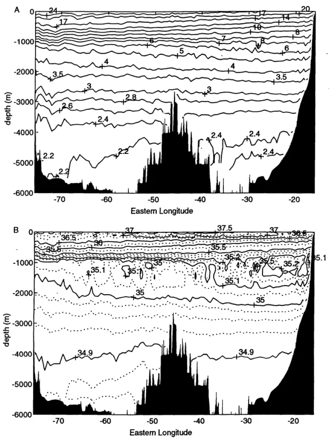
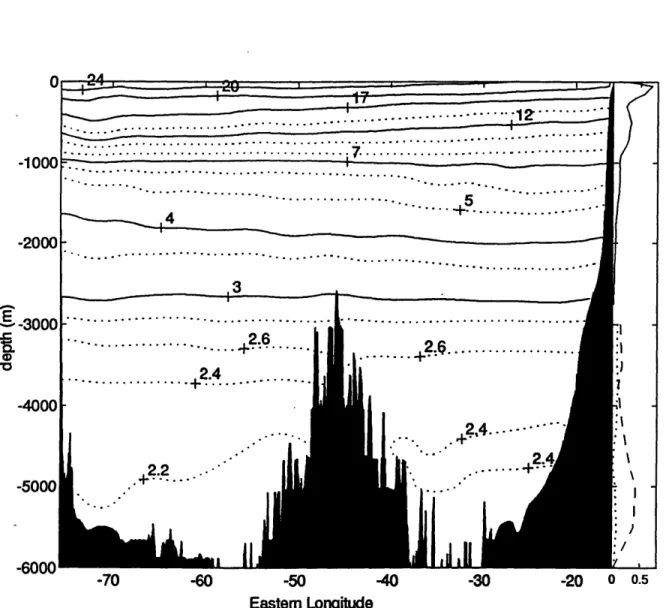
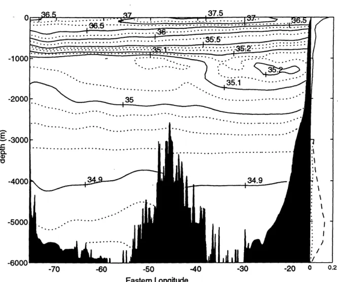
The 2-db temperature, salinity, and oxygen data have been smoothed with a binomial filter and then linearly interpolated (Mamayev et al., 1991) as required to the standard levels (Table 1.1). When the CTD did not reach the bottom, to enable interpolation to all available standard depths, linear vertical extrapolation were used to estimate one more standard depth from the last two interpolated depths. Figure 1.2 A, B and C present distributions of temperature, salinity, and oxygen for the 1992 Hesperides Section.

(20)

E 3000 -70 -60 E -50 astem Longitude .Az .37.5 3 .. .. ... ... ... °~~. .. . .. . .. . . .. .. .°° ° °o° °° °.•° °° = 35. - ., 35.~ 5:'C 35F ... -- ° ..- ... . . .. . . .°.. .... ... 34.9 • . °° ° * * ° °• -60 -50 Eastem Longitude -40

Figure 1.2: Distributions of A) Temperature (OC), B) salinity (pss) C) Potential temperature (OC), and D) oxygen (ml 1-') for the 1992 Hesperides Section

-40 -20 E "-3000 -C -or -4000 -5000 -6000 -70 -20 k_

(21)

C 0 12 -1000 .7 ,7 -2000 E _-3000 2.5 2.5 U) -4000 -5000 1. -6000 -70 -60 -50 -40 -30 -20 Eastem Longitude -1000 -2000 3000 -(7 -70 -60 -50 -40 Eastem Longitude -20

(22)

Chapter 2 Comparison over Time of Temperature and Salinity

2.1 Introduction

The objective of this research is to investigate the climatic variations of tem-perature and salinity over the tropical Atlantic Ocean from the surface to 6000 m depth during the last 35 years. All three available cruises have been done at the nominal latitude of 24.50N. However, the 1981 cruise started on the African Conti-nental shelf at 27.9N and angled southwestward to joint 24.50N at 24.30_{W due to} the Sahara war which was close to the coast at 24.50N.

The nominal station spacing in the IGY survey was 185 km. On the Atlantis II, the spacing varied between 50 and 80 km with shorter spacing when the stations were over the continental slopes and the Mid-Atlantic Ridge. The same criteria were used for the Hesp"rides survey, but the spacing was more regular, between 58 and 67 km. Therefore, in order to compare the variables from the different cruises directly it is necessary to interpolate all the data onto a set of common geographic locations. The data were interpolated onto a two dimensional grid at 24.50N. The horizontal spacing chosen was 0.50 of longitude. This corresponds approximately to 50 km at

(23)

this latitude (0.5 x 60 x 1.85 x cos(24.5) = 50.5 km). The data were placed vertically onto a set of 35 standard depths, defined in Table 1.1

2.2 Methodology

In order to choose a scheme of interpolation, we compared spline interpolation and objective mapping, two methods which could reasonably be used. Here we de-scribe how their advantages and disadvantages led to the decision to use one of them for this work. Between the results of the two methods, discrepancies are within the expected error in all regions except the boundaries. Cubic spline is simpler to use but the advantage of calculating expected errors made objective mapping the most suitable method of interpolation for this analysis.

2.2.1 Spline interpolation

The spline interpolation (Ahlberg et al. 1967) assumes the existence of a function y = f(zx) whose value is known at a set of ax points, a = xo < x1 < ... <

z, = b, regularly or irregularly spaced. The cubic spline is the cubic polynomial f(s) that is continuous in the interval [a, b], has continuous first and second derivatives, and passes through the points f(zi) (i=0,n). The interpolating cubic spline defines a separate cubic polynomial for each interval xi- 1

<

x < zx, or a total of n polynomials for the n+1 points. We can write the polynomial equation take derivatives and , at each data point equate the first and second derivative of the left-side polynomial to those of the right-side.

(24)

Following Thompson (1984), writing the Taylor series for the cubic polynomial for interval i, expanded about the point zi

y() = y + (x - )y + (x - x) y /2 + (x - (y+- )/6h (2.1)

yl and y' stand for the first and second derivatives evaluated at x = xi, and the third derivative has been replaced by its divided difference form, which is exact for a cubic function (Bevington and Robinson, 1992). At x = xi, we have y = yi, as required. Setting x = zi+l = xi + h it is possible to solve the equation

y(Xi+1) = Y~ + (X;+1 - X)y + (X,+1 - X,)2 y'/2 + (xzi+ - xs)(y,+A - y; )/6h (2.2)

to obtain

(yi+1 - yi) = hy' + h2 [2y' + y '+,]/6 (2.3) Repeating the calculation, using the equation for y(x) in interval i-1 and requiring that y(x) = y(xz) at the i data point we obtain

(yi - yi-1) = hy,-1 + h2 [2y" 1 + yj ]/6 (2.4)

To establish continuity conditions at the data point, we equate first and second deriva-tives at the boundaries x = xi and x = xi-1. The use of the divided difference form for the third derivative assures continuity of the second derivative across the boundaries and gives the spline equation

I II II

Yi-1 + 4 y, + y,-i = Di (2.5)

with

Di = y [yi+l - 2y; + yil]/h2 (2.6) These equations can be solved for the second derivatives y', as long as the values of y" and y, are known. If those values are set to 0 the natural splines are obtained.

(25)

In our case we have used natural splines for the interpolation. The fitting by cubic splines was done from the longitude of the western-most to the eastern-most station, for each of the 35 standard depths. After fitting, the function was evaluated every 0.50 of longitude. Below 2750 m (standard depth number 24) the North Atlantic is separated by the Mid-Atlantic Ridge in two basins, the North American basin and the Canarias basin. Since the behavior of the basins is different, the fitting was done separately for each.

The set of data obtained after the gridding is for Hesperides 1992 from 75.50_W to 160W, for Atlantis 1981 from 75.50_{W to 13.5}0_{W and IGY 1957 from 75.5}0_{W to} 16.50W. Atlantis-II data, due to the deviation of the track from 24.50N east of 24.50W, only compared with the other sections west of 24.50W. For comparison we only have computed west of this longitude. After gridding for the three cruises, we calculated the differences on the common area:

* 1992-1981: Subtracting 1981 data from 1992 between 75.50W and 24.50_W. * 1981-1957: Subtracting 1957 data from 1981 between 75.50W and 24.50W. This

comparison was also done by Roemmich and Wunsch (1984) using objective mapping.

* 1992-1957: Subtracting 1957 data from 1992 between 75.5 and 16.5 oW.

Because the grid-point temperature differences exhibit large variations due to the presence or absence of eddies during the different surveys, a horizontal gaussian filter of e-folding scale of 300 km has been applied to the temperature differences at each depth.

Behavior of the boundaries

When we apply the gaussian filter at the boundaries, we extend the temper-ature difference matrices in an unbiased way with zeros past the boundaries so that

(26)

smoothed temperature differences are obtained up to the western and eastern bound-aries as well as in the Mid-Atlantic Ridge.

Figure 2.1 A, B and C present temperature differences for 1981-1957, 1992-1981 and 1992-1957 obtained with this methodology.

For salinity we have done calculation similar to those for temperature, fitting by cubic splines at each standard depth and using a gaussian filter of the differences. Figure 2.2 A, B and C present salinity differences for 1981-1957, 1992-1981 and finally 1992-1957.

(27)

...

...

- 0 , _~. I . .. .... -100_-200 ... -300 -400 -in--1000 _-6000.. . .. . ... t~ -700060 _{j-. K -t} 3 ... ... ... -3000 -" xr expandedt~ ca vertcal _-0.05 _-- _{-0 25~:}_{:''s::::::;S:;;} -0.0250 x---5 -000 _E _x., ~~" -6000 -6 70 -50 40 -3 Easer Logiud

Figue 21: Dffeenc of empratue a 2401:O usng slin fitingandintepoltin

vausec .'flniue aawr mote sn asin itro -odn

scal of300km. iffrenes ere alclatd fr A)981195 B)1992198, ad C 1992195. Vauesarein ". Sadig inicaes psitve iffeenc.Th topplo ha

(28)

-50 Eastern Longitude -100 -200 -300 -400 -3000 E U)

(29)

0 -10 -200 -300 -400 -0.25 -1000 .025 -2000 -3000

_

---

0.025

-4000 -0.025 S-0.025 -5000 -6000 -70 -60 -50 Eastern Longitude -40 -20

(30)

e -1 -4000

7

-0.5 -0.5 -0.5 -5000 .5 -6000 -70 -60 -50 -40 -30 Eastern Longitude

Figure 2.2: Difference of salinity at 24.50N using spline fitting and interpolating values each 0.50of longitude. Data were smoothed using a gaussian filter with of 300 km of e-folding scale of 300 km. Differences were calculated for A)1981-1957 B) 1992-1981, and C) 1992-1957. Values are in pss x 100. Shading indicates positive difference. The top plot has expanded vertical scale

(31)

-2.5f

-70 -60 -50 Eastern Longitude -1000 -2000 -3000 -4000 -4000 -5000 -6000 -40

(32)

S112

-70 -60 -50 -40 -30 -20 Eastern Longitude -400 -3000 E (D V

(33)

2.2.2 Objective mapping

The technique for the objective mapping is based on a standard statistical re-sult, the Gauss-Markov Theorem, which gives an expression for the minimum variance linear estimate of some physical variable given measurements at a limited number of data points (Bretherton et al. 1976). Objective mapping has been used by a num-ber of physical oceanographers, (e.g.., Roemmich (1983), Wunsch(1985) and (1989), Fukumori et al. (1991)); I will give just the basic derivation applied to a hydrographic section.

We are presented with a section of hydrographic stations, in the case of the Hesperides cruise 101 stations, located in a set of longitudes r= [ri]. For each standard depth we have a data series of variables such as temperature, salinity, etc. Let's call them {T} = T(r,) where i goes from 1 to the number of stations sampled at that depth.

Because of sloping topography at the boundaries and the Mid-Atlantic Ridge, not all the depths will have 101 values. Below 3500 m, we will have two data series, one for the North American Basin and another for the Canary Basin. We denote the total number of stations by N.

In the case that the mean, < T >= 0, (usually approximation is obtained by removing the sample mean value at each standard depth), the covariance matrix of T at the data point is given by:

{Ri3} = R(r,,rj) = {< T T >} (2.7)

where i and j go from 1 to N. The size of this data covariance matrix is an N x N. If T is spatially stationary or homogeneous its second moments depend only on the separation of the evaluation points.

(34)

The set r = {ri} contains the points where the values of Ti are required. In this case the points will be from the western coastline (75.50W ) to the eastern coastline (160_W) with an interval of 0.50. The number of interpolated values, M, is 120. The objective is to estimate the variable value ''() from observations. S(r) = T(r,) + n(r,) where n is the observational noise, with zero mean and known covariance.

< n(r) n(r3) >= N(r - rj) (2.9)

Then R(rk, ri) is the covariance matrix of T at the interpolation points with its value at any data point. The field we seek to map has the statistics given by R. Suppose the noise is uncorrelated with the value of T:

< T(ri) n(rj) > = 0 all i,j (2.10)

Suppose further, that the interpolated value is a weighted average of the observations:

T(k) = B(k, rj) S(rj) = B(ik) S (2.11)

where B is an M x N matrix. We then evaluate the variance of the difference between the correct value at rk and the interpolated value

P = < (T(,) - T(ik))2 > = < (B S - T(i)) 2 > (2.12)

The Gauss-Markov theorem states that the minimum of this difference is reached when B is chosen as

B = R(k,r) [R(ri, rj) + N(r, r)i-1 (2.13)

and the minimum possible expected error is,

Pmin = R(rk,k) - R(rk, ri) [R(ri, j)+ N(ri,r r)] RT(rr, ,k) (2.14)

One of the important uses of the mapping is the determination of a mean value. Let the measurements of a variable, temperature for example, be denoted by yi and

(35)

suppose that each is made up of a large-scale mean, m, plus a deviation from that mean of 08 (Wunsch, 1989), so that we can write

m + 0, = y;, i = ItoN (2.15)

or

Dm + 0 = y, DT = [1, 1,..1] (2.16)

We seek a best estimate, mk, of m. Suppose an a priori estimate of the size of m exists, and is called ino, i.e. < m2 >= m. If R is the spatial covariance of the measured

field about its true mean, the best estimate of the mean (Liebelt, 1967, Eq. 5-26) can be written

M= [ + DTR-1D]-DTR-lY

1 DTR-ly _(2.17)

+ DTR-1D

(DTR-1D is a scalar). The expected error of the estimate is

E = (1 + DTR-1D)-I

ino

1

= (2.18)

-1 + DTR- 1D

the goal of the analysis is to retain and separate the large-scale time-averaged features from the time-dependent features and errors.

Objective mapping requires a statement of the expected a priori measurement error, and mapped field covariances (Bretherton et al. 1976). We must define what is signal and what is noise, the variance of the data contains the signal variance as well as the noise variance. We assume that the noise includes two components: the first component, n., is the variation caused by mesoscale eddies; the second one ni is the variance caused by the local measurement error (including errors due to navigation, interpolation, instrumentation, etc) (Wunsch, 1989). Assuming the component are

(36)

independent of one another, the total variance < T2 > can be written,

< Tj' > =< a> + < n > + < , > (2.19)

where the total variance of the data is given by the signal variance < sa >, the eddy noise variance < n, > and the intrinsic noise variance < n2 >.

Signal and eddy noise covariances will be modeled by a gaussian covariance function; ni is modeled by a delta function, n, on the other hand, has a finite correla-tion distance, but this distance is smaller than the correlacorrela-tion distance of the signal we are trying to map.

To estimate the e-folding scale of these distributions I have calculated the correlation function. I will describe the calculations done for the 1992 cruise. Because of the different station spacing, we have used 3 sets of data: the Canary Basin between station 11 and 41; the Mid-Atlantic Ridge between stations 42 and 64 and the North American Basin between stations 65 and 96. The distance between stations was 58 km for the Mid-Atlantic Ridge region and 67 km on the other two regions. To estimate the dominant length scales of the eddies we compute the spatial correlation function < T'(x)T'(x + Ax) > (2.20) P(z) = ₍_<_(T'(x))2 _><_{(T'(x + Ax))}2_> (2.20)

where T' are the data values once we have subtracted the linear trend.

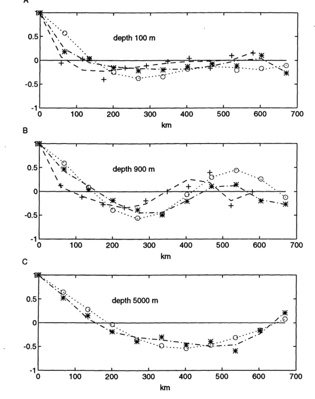
We have computed the function for Ax = 0, 58, 67, 116, 134,... km. Figure 2.3 A, B and C present the values for depths of 100, 900 and 5000 m. For these plots we can see short scale correlations over the Mid-Atlantic Ridge for the shallower plots (there are no 5000 m depths over the Mid-Atlantic Ridge). The zero-crossing distance is between 75 and 100 km. In deep water, for the eastern basin, this distance is around 150 km, and between 150 and 200 km for the western basin. We have taken a value of 175 km for e-folding distance of the gaussian noise covariance. The scale is perhaps somewhat too large, but it has been chosen to make the plots smoother.

(37)

-0.5 + 1 I I I I f I 100 200 300 400 km 0.5 \ ; \ " ., O--0.5 -1 0 100 depth 900 m .7 * , -- _ . , °" ~~t_ 0*\ _.I 200 300 400 + xI 600 500 700 km 0. -0. 100 200 300 400 500 600 700 km

Figure 2.3: Correlation function (equation 2.20) for the North American Basin (o), Mid-Atlantic Ridge(+) and Canary Basin (x) for some depths A) 100 m, B) 900 m and C) 5000 m 500 600 700 1 .5- K'.. depth 5000 m .5. *...- .. .1 I I

(38)

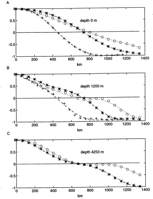
Same as Fig 2.3 but with eddy motion filtered out was done for the the signal correlation function. Figure 2.4 A, B and C show the signal correlation function for depths of 0, 1200 and 4250 m. We have taken an e-folding scale of 400 km for the signal covariance at all depths. The zero-lag covariances have been estimated following the method described by Fukumori et al. (1991). Let Tj the data at station j at a certain depth, with signal si, eddy noise n,j and intrinsic noise nij

Tj = sj + n,j + ij (2.21)

The mean square difference from a neighboring station (j + 1) is,

< (Tj - Ti+~) >=< (sj - sj+l +

nj

-

n2j+1 +

-- ij+1) >

~j

=< (sj - sj+x + nej - nej+1)2 > +2 < nf > (2.22)

where we have assumed the intrinsic noise is uncorrelated over the distance and has uniform variance. If the signal and the eddy noise have much longer correlation distances than the station separation, it is possible to neglect the first term on the right hand side of equation 2.22 with respect to the second term which yields

< (Ti - Tj+ )2 >- 2 < n > (2.23)

In the same way, let < (Tj - Tk)2 _{>L denote the mean square difference of data}

between two points, j and k, separated by L km, then

< (Tj - Tk)2 >L = < (Sj - Sk + lj - nk + i, - nik)2 >

2 < s>-2 < jS_k>L +2 < n > -2 < nenek >L +2 < n> (2.24)

If the signal s, has a length scale much longer than L, the second term will be similar to the first and they will partially cancel. Using a distance of 400 km, these two terms cancel; if the eddy noise covariance has a length scale smaller than that distance, then equation 2.24 will be approximated by

(39)

5- . depth 1200 m -0u " " . .5 - ₀ O.0 5 II 0 200 400 600 800 1000 1200 1400 km "i.- 0&1 5 ". depth 4250 m 0-- -' • " 0". 0* .1(1 5 _I.I _p _p )K-. "0 120 40 0 200 400 600 800 1000 km

Figure 2.4: Signal correlation function (same as Fig 2.3, but with eddy motion filtered out) for the North American Basin (o), Mid-Atlantic Ridge(+) and Canary Basin (x) for depths A) surface , B) 1200 m and C) 4250 m

0. -0. 0., -0. __ --I 1200 1400

(40)

Signal variances have then been calculated by equation 2.19.

For computing the expected difference for a spatial separation, we have taken the data set between station 11 and station 96, where the spacing is homogeneous. The distance between a station and the neighboring one is less than 70 km. Due to the different behavior of the deeper part of the North American and the Canary Basins the variance calculations for depths below 2750 m (the depth of the shallowest station in the Mid-Atlantic Ridge) have been computed separately for each basin.

At 900 m the signal variance is smaller than the noise variance. The mapping is practically using the mean temperature value for most of the section. In the Canary Basin, values below 4750 are scarce. For the computations of the eddy noise variance we have used a distance of 200 km, and for the intrinsic noise a value of 0.0040C at 4750 m and 6000 m. On the Western Basin at 6000 m we have used a value 0.002°C. These values are slightly higher than the value for instrumental noise of a Mark III CTD given by Millard et al., 1990.

The variances used are:

1 < ? > = < T > - < ( j) >400Km (2.26) 22 2 1<(Ti 2 (2.27) <n>= < (T,- j) >4o,, -400 < > 1 < ni > < (T, - Ti+1)2 >70Km (2.28)

The variance of the temperature signal (s), eddy noise (n.) and measurement noise (n?) are summarized in Table 2.1 at the standard depths for all the North Atlantic Basin shallower than 2750 m., Table 2.2 below 3000 m for the North American Basin and Table 2.3 below 3000 m for the Canary Basin.

The variance of the salinity signal (s,), eddy noise (n2) and measurement noise (n?) are summarized in Table 2.4 at the standard depths for all the North Atlantic

(41)

depth si ne n (m.) 0C 0C 0C 0 2.41 0.33 0.17 50 1.94 0.81 0.64 100 1.54 0.73 0.65 150 1.10 0.69 0.71 200 1.04 0.44 0.47 250 1.15 0.29 0.30 300 1.34 0.23 0.25 400 1.59 0.29 0.24 500 1.50 0.35 0.24 600 1.17 0.33 0.24 700 0.85 0.33 0.24 800 0.50 0.28 0.23 900 0.19 0.24 0.19 1000 0.22 0.15 0.16 1100 0.36 0.10 0.23 1200 0.45 0.10 0.21 1300 0.46 0.11 0.14 1400 0.43 0.10 0.12 1500 0.37 0.08 0.11 1750 0.22 0.06 0.06 2000 0.13 0.05 0.05 2250 0.09 0.04 0.04 2500 0.06 0.03 0.03 2750 0.03 0.02 0.03

Table 2.1: Signal (si), eddy noise (n,) and measurement noise (n1) square root

vari-ances for mapping temperature data at the indicated depth at 24.5 "N for all the North Atlantic Basin shallow than 2750 m. Data are given in 'C

(42)

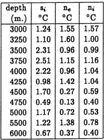
depth si ne ni (m.) OC OC OC 3000 2.57 1.31 2.97 3250 3.42 1.55 2.62 3500 3.59 1.90 2.68 3750 1.56 1.53 1.96 4000 2.70 1.70 1.56 4250 3.65 2.39 1.74 4500 4.92 3.31 1.69 4750 5.48 4.48 1.87 5000 6.15 7.15 2.96 5500 5.62 6.20 3.75 6000 1.17 0.11 0.20

Table 2.2: Signal (si), eddy noise (ne) and measurement noise (ni) square root vari-ances for mapping temperature data below 3000 m at 24.5 ON for the North American Basin. Data are given in 0C x 10-2

depth si ne ni (m.) oC OC OC 3000 1.24 1.55 1.57 3250 1.10 1.60 1.00 3500 2.31 0.96 0.99 3750 2.51 1.15 1.16 4000 2.22 0.96 1.04 4250 0.98 1.42 1.04 4500 1.70 0.27 0.59 4750 0.49 0.13 0.40 5000 1.17 0.72 0.53 5500 1.22 1.38 0.78 6000 0.67 0.37 0.40

Table 2.3: Signal (si), eddy noise (n.) and measurement noise (ni) square root vari-ances for mapping temperature data below 3000 m at 24.5 ON for the Canary Basin. Data are given in oC x 10- 2

(43)

Basin shallow than 2750 m., Table 2.5 below 3000 m for the North American basin and Table 2.6 below 3000 m for the Canary Basin.

Since the distance (r, - r3) in our covariance functions is given in longitude

degrees, we have used 40 and 1.750, which is equivalent to 400 and 175 km (at this latitude l1x 60' x cos(24.5)=101 km). Then the covariances are:

R(r - r) = < s? > exp(-(r - r)/4 2 ) (2.29) N,(ri - r) = < n > exp(-(r, - ri)2

/1.752 ) (2.30)

Ni(ri - r,) = < n? > 6(ri - rj) (2.31)

Behavior of the mapping function on the boundaries

As you approaches the boundaries not all data point are available and the mapping function given by equation 2.13 becomes one sided. The mapping function reduces the variability of the data, errors increase and the expected value tends to the mean.

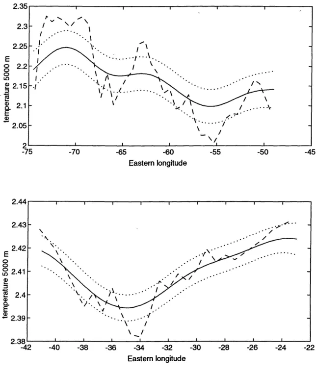
Figure 2.5 presents values of raw data and mapped data with its error at 5000 m depth in the North American and Canary Basins. It is possible to see the different behavior of the temperature in both basins and the associated error. The uncertainty is around 0.040C in the North American Basin and only about 0.0050_{C in the Canary} Basin. Errors are slightly increased near the boundaries. In this case the mapped values are practically within the sampled area. Near the boundaries of the basins where due to the irregular topography there are some gaps, we have mapped values outside the sampled area.

The mapping values of temperature for the 1992 cruise are presented in Figure 2.6. The expected error in the temperature mapping (Bretherton et al. 1976) as a function of depth is shown on the right side. Below 3000 m, the error is given sepa-rately for the North American and Canary Basins. These errors have been computed

(44)

depth si ne ni (m.) pss pss pss 0 4.21 1.93 1.24 50 3.36 1.18 0.99 100 2.10 0.90 1.11 150 1.12 0.73 1.31 200 0.93 0.46 0.81 250 1.47 0.39 0.56 300 1.96 0.33 0.44 400 2.40 0.43 0.38 500 2.09 0.49 0.36 600 1.42 0.42 0.35 700 0.91 0.42 0.34 800 0.49 0.34 0.34 900 0.36 0.29 0.25 1000 0.42 0.22 0.24 1100 0.50 0.20 0.50 1200 0.59 0.18 0.39 1300 0.60 0.19 0.25 1400 0.59 0.19 0.22 1500 0.51 0.17 0.19 1750 0.35 0.12 0.10 2000 0.22 0.07 0.06 2250 0.15 0.04 0.04 2500 0.10 0.03 0.03 2750 0.06 0.02 0.02

Table 2.4: Signal (si), eddy noise (n,) and measurement noise (n,) square root vari-ances for mapping salinity data at the indicated depth at 24.5 ON for all the North Atlantic Basin shallow than 2750 m. Data are given in pss x 10-1

(45)

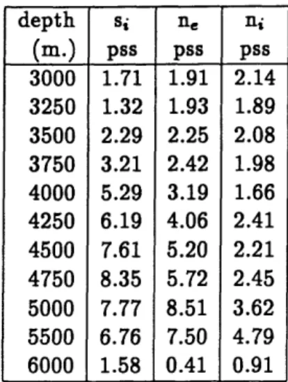
Table 2.5: Signal (si), eddy noise (n,) and measurement noise (ni) square root vari-ances for mapping salinity data at the indicated depth at 24.5 ON Below 3000 m for the North American Basin. Data are given in pss x 10- 3

depth si ne ni (m.) pss pss pss 3000 2.28 1.18 1.57 3250 0.70 1.57 1.08 3500 1.25 0.84 0.87 3750 1.73 1.23 1.30 4000 1.23 1.11 1.00 4250 0.49 1.28 0.99 4500 1.28 0.57 0.78 4750 0.47 0.34 0.57 5000 0.98 1.05 0.63 5500 1.22 1.61 0.76 6000 0.39 0.51 0.85

Table 2.6: Signal (si), eddy noise (n.) and measurement noise (ni) square root vari-ances for mapping salinity data at the indicated depth at 24.5 °N Below 3000 m for the Canary Basin. Data are given in pss x 10- 3

depth si ne ni (m.) pss pss pss 3000 1.71 1.91 2.14 3250 1.32 1.93 1.89 3500 2.29 2.25 2.08 3750 3.21 2.42 1.98 4000 5.29 3.19 1.66 4250 6.19 4.06 2.41 4500 7.61 5.20 2.21 4750 8.35 5.72 2.45 5000 7.77 8.51 3.62 5500 6.76 7.50 4.79 6000 1.58 0.41 0.91

(46)

2.35 2.3 2.25 2.2 2.1 2.05[ 21 -7 I II -. \/ \ S"'.". _. . /'.. . E . . " \. .. o II I I I • -'60.' I "" "" \ 4-- "" " .. ... ... I I I I -60 Eastern longitude -40 -38 -36 -34 -32 Eastern longitude -30 -28 -26 -24 -22

Figure 2.5: 1992 cruise raw data (dashed), mapping data (solid) plus/minus the error in the mapping (dotted) for A)North American basin and B) Canary Basin. data are in oC. -50 -45 2.44 2.43 2.42 2.41 2.39 2.38 -42 \ ...

.

-.

,

.

' '' I I I I I I I I I 15 5 2.4F

(47)

by the square root of the diagonal of P, m in (2.14) . The highest values appear at 50

m, where the highest eddy noise variance was found (Table 2.1). Between this depth and the middle of the thermocline (- 850 m), the error decreases to 0.2°C. Below -2000 m, the expected error is less than 0.050C, for all the cruises. Errors in the Canary basin are less than 0.020C while in the North American one they are between 0.01 and 0.04"C with the highest values appearing between 5000 and 5500 m.

Salinity mapping has been done in the same way as the temperature mapping, we present in Figure 2.7 salinity mapping for the 1992 cruise including the expected error for this mapping. Expected errors in salinity are largest at the surface and reduce with depth.

Calculations of covariances and mapping were performed for 1981 and 1957 datasets the same as it was described for 1992 dataset. After this interpolation to a common grid, we have calculated the differences for the three cruises for the same extension we did for spline interpolation. Figure 2.8 A presents the temperature dif-ference between the 1981-1957 cruises. Figures 2.8 B and 2.8 C give the temperature differences from 1992-1981 and 1992 and 1957.

The expected error of the differences is the sum of the expected errors of the mapping values for each map. We have adding the values of P,mi in equation (2.14) for each set of data and taking the square root of the diagonal. On the right side of the figures the expected error in function of depth is presented. Figure 2.9 A, B and C presents the difference in salinities for 1981-1957, 1992-1981 and 1992-1957. Expected errors have been calculated in the same way as for temperature.

(48)

... .. .12... ---" . .. ... ...7 .. . ... . ... ... .. .. ... . .... . . .. .' ' .'4 . ... . . . . .... . ..5 ... . . .. . 4.... ... ... _...-... • ... 4° ° °. . ° '' '. . .° '

...

.I

...

.6. -I-.

11

-50 -40 Eastem Longitude

Figure 2.6: Temperature values for the 1992 cruise using objective mapping, Data are in OC. The expected error in the temperature mapping in function of depth is shown on the right side. Below 3000 m, the error is given separately for the Canary (dotted) and North American (dashed) Basins and values are multiplied by 10). Expected errors are in °C. -1000 -20001 -3000 0, -4000 1 -5000 -6000 2.2 | i :1 I.I *1 -0 . -70 -60 -30 -20 . .. .... •... ... 2. ... +-!,~. ...

(49)

6-5

U

37.5

- --.-.-0 7-r . .. ...

-....000 ..

-70 -60 -50 -40 -30 -20 0 0.2

.basins

and values are multiplied by 25). Data are in pss...

-2000 - 35 '... .- .. -4000 134.9 -5000 -6000 -70 -60 -50 -40 -30 -20 0 0.2 Eastem Longitude

Figure 2.7: Salinity values for the 1992 cruise using objective mapping. The expected error in salinity mapping in function of depth is shown on the right side. Below 3000 m, the error is given separately for the Canary (dotted) and North American (dashed) basins and values are multiplied by 25). Data are in pss.

(50)

-100 -200 -300--400 M -1000 -2000 -0.0 -- 3000 - : -4000 -0. 5 0.025 -5000 -70 -60 -50 -40 -30 0 1 Eastern Longitude

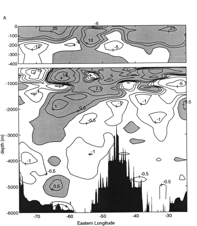
Figure 2.8: Difference of temperature by objective mapping, A) 1981-1957, B) 1992-1981 and C) 1992-1957. Data are in OC. The expected error in the temperature difference in function of depth is shown in the right side. Below 3000 m, the error is given separately for the Canary (dotted) and North American (dashed) basins and values are multiplied by 10). Expected errors are in C. The shaded indicates positive difference. The top plot has expanded vertical scale.

(51)

k -0

U

V

A

i

-70 -60 -50 -40 -30 0 Eastern Longitude -20( -30( __ C_

(52)

-70 -60 -50 -40 -20 o

(53)

-100--2 0 0 0 .5 -300 \ -400 -1000

-2000

05 -0.5 I

-3000

-0.

5

-70 -60 -50 -40 -30 0 20 Eastern Longitude

Figure 2.9: Difference of salinity by objective mapping, A) 1981-1957, B) 1992-1981 and C) 1992-1957. Data are in pss x 100. The expected error in salinity difference in function of depth is shown in the right side. Below 3000 m, the error is given separated for the Canary (dotted) and North American (dashed) basins and values are multiplied by 25. The shaded area indicates positive differences. The top plot has expanded vertical scale.

(54)

B E ,c a. "0 -70 -60 -50 -40 -30 0 20 Eastern Longitude

(55)

iAN -1 10. 1 -0.5 -50 -40 Eastern Longitude 0 -100 -200 -300 -400

\

I -20 0 o -70 -60

(56)

2.2.3 Discussion

I have compared the use of cubic spline interpolation and objective mapping to interpolate the data to a regular grid. The most significant differences between the two methodologies are that the spline interpolation with the gaussian filter gives a large scale vision of the features, but smooths over the small scale features, and that the maximum values are reduced in most of the cases.

The behavior of the gaussian filter on the boundary data is to smooth these values and tends to reduce the differences in this region. The objective mapping also smoothes the values and reduces the differences in the boundaries, but to a lesser extent; so that the objective mapping slightly increases differences relative to the gaussian filter.

This effect can be seen in the eastern boundary 1992-1957 difference (Fig 2.1 C, Fig 2.8 C). In the North American Basin, we can find most of these effects on the two boundaries (Continental shelf and Mid-Atlantic Ridge) and at the bottom of the basin. Even when we are looking at the large scale effects, I think it is convenient maintain these boundary differences.

Due to the behavior of polynomial functions, when the fitting has to be ex-tended outside the sampled area, values calculated by splines change very quickly. In these regions, values given by objective mapping are more realistic than values given by spline interpolation.

There is a high degree of similarity among cubic spline smoothing with a gaussian filter and objective mapping methods using the convenient parameters. The discrepancies are within the expected error in all regions but the boundaries.

(57)

* fast, and does not need much memory

* there exist fast routines in software, i.e., in packaged form.

* it doesn't require any a priori knowledge about the data or the measurement error.

* gives the real value on the sampled locations

* the results are reasonable, discrepancies are within the expected error, in this application.

Disadvantages of using cubic spline

* there is no estimate of uncertainties

Advantages of using objective mapping

* extrapolated values near the continental slopes or the bottom topography are better determined.

* the most important advantage is the expected error given by the method in the form of an error map.

In this case, when we are attempting to perform data comparison, the er-ror maps are a fundamental requirement. Without the expected erer-rors, we can not recognize whether or not the differences are significant.

Disadvantages of using objective mapping

* It requires a lot more work and computing time, matrices are usually big and demands large computer memory.

(58)

* It requires previous knowledge of the covariance functions or assuming the cor-relation matrices.

* not available in packaged form. One must build it from the start.

The possibility of calculating expected errors has made objective mapping the most suitable method of interpolation for this analysis.

Climatic changes in temperature and salinity in the subtropical North Atlantic