Colliding bubble universes in eternal inflation

MASSACHUSETTS INSTITUTE OF TECHNOLOGY Colliding bubble universes in eternal inflation

JUN

0

8

2011

Nathaniel C. Thomas

L

BA R I

E

S

Submitted to the Department of Physics

in partial fulfillment of the requirements for the degree of Bachelor of

ARC9W'ES

Science at the Massachusetts Institute of Technology

@2011 Nathaniel C. Thomas

CJvne

'7o1]

All rights reserved.

The author hereby grants to MIT permission to reproduce and to distribute publicly paper and electronic copies of this thesis document in whole or

in part. Signature of Author -Department of Physics May 18, 2011 Certified by Alan H. Guth Thesis Supervisor, Department of Physics Accepted by

Professor Nergis Mavalvala Senior Thesis Coordinator, Department of Physics

Colliding bubble universes in eternal inflation

Nathaniel C. Thomas

Submitted to the Department of Physics

in partial fulfillment of the Requirements for the Degree of

BACHELOR OF SCIENCE

at the

MASSACHUSETTS INSTITUTE OF TECHNOLOGY

May 18, 2011

Abstract

We briefly summarize arguments for inflation and discuss eternal inflation. We then discuss the motion of domain walls and null shells that form in two-bubble collision processes in both the global and in-bubble FRW coordinates. Comments are made regarding possible observational signals.

Thesis Supervisor: Alan H. Guth

Acknowledgements

Many thanks to Professor Alan Guth for being a fantastic thesis advisor. Thanks to Dr. Ben Freivogel and Professor Raphael Bousso for helpful dis-cussions. Thanks especially to my parents.

Contents

1 Introduction 8

2 Inflationary Cosmology 9

2.1 Three cosmological problems . . . . 9

2.1.1 Horizon problem . . . . 9

2.1.2 Flatness problem . . . . 10

2.1.3 Relic problem . . . . 10

2.2 Microphysics of inflation . . . . 11

2.3 Generating the primordial density perturbation . . . . 13

2.4 Comments about inflation . . . . 13

3 Eternal inflation 14 3.1 Coleman-de Luccia Instanton . . . . 14

3.2 False vacuum eternal inflation versus slow roll eternal inflation 15 3.3 Eternal inflation and the landscape of string theory . . . . 15

4 Bubble collisions 16 4.1 Spacetimes with SO(2, 1) symmetry and the hyperbolic Birkhoff theorem . . . . 17

4.2 Bubble collision spacetimes . . . . 18

4.2.1 Hyperbolic Schwarzschild . . . . 19

4.2.2 Hyperbolic Schwarzschild-de Sitter . . . . 19

4.2.3 Hyperbolic Schwarzschild-anti de Sitter . . . 21

4.3 Assumptions . . . . 22

4.5 Motion of domain walls . . . . 27

4.5.1 Israel junction conditions . . . . 27

4.5.2 Flat

/

flat collisions . . . . 29 4.5.3 Motion of the domain wall for general collisions . . . . 37

4.5.4 Note on Raychaudhuri's Equation . . . 41

5 The view from inside 42

5.1 Null shells in flat background and interior . . . 42

5.2 Null radiation shell in de Sitter bubbles . . . 45

6 Observational Signatures 46

7 Conclusions 47

7.1 Status of Observations . . . 47

List of Figures

1 Potentials for the scalar field in old inflation (blue) versus new inflation (purple) . . . . 12 2 Conformal diagrams for Minkowski and hyperbolic Schwarzschild

spacetimes (each point corresponds to a 2-hyperboloid) . . . . 20 3 Conformal diagrams for dS and hyperbolic Schwarzschild dS

spacetimes (each point corresponds to a 2-hyperboloid) . . . . 21

4 Conformal diagrams for AdS and hyperbolic Schwarzschild

AdS spacetimes (each point corresponds to a 2-hyperboloid) 22

5 A spacetime diagram of a two-bubble collision in a frame in

which the bubbles are nucleated simultaneously. The regions have the following properties (using the notation of the metric in Equation 4.1): (1) background metastable vacuum state

(A > 0, so = 0), (2) left and (3) right bubbles outside of the

future lightcone of the collision (so = 0, A variable), (4) left and (5) right sides of the domain wall (so

#

0 in general, A

variable) . . . 23

6 The shape of the double well potential considered in [17] . . . 25 7 Figure illustrating conservation of energy-momentum at a point

of collision. Time flows upward. Each line represents a sheet of matter or radiation that is entering or exiting the collision point. The 3s refer to the velocity of sheet one sheet in the reference frame of another sheet . . . . 26 8 Motion of the domain wall separating two Minkowski bubbles

9 Form of the effective potential governing the motion of the domain wall in the non-extremal case . . . 40

10 Form of the effective potential governing the motion of the domain wall in the BPS case . . . 40

11 Sketch of null shell radius dependence on T as seen from inside the bubble for 6 = 0 in a flat background and bubble interior. 44 12 Sketch of null shell radius dependence on 0 as seen from inside

the bubble for varying r (r is smallest for the blue curve and increases on higher curves) in a flat background and bubble interior. . . . 44

1

Introduction

With the discovery of galaxies beyond the Milky Way, astronomers increased the size of the known universe by orders of magnitude. The theory of infla-tion demands another radical increase in the maximum known scale: Instead of only a single universe, the theory implies the existence of a large (possibly infinite) number of other "bubble universes," born from unstable primordial energy. This collection of bubble universes is called the "multiverse." Infla-tionary theory requires more than simply adding more space to the universe because (due to effects from general relativity) these bubble universes are in general causally disconnected from each other; we can never see most of these universes or be seen by any scientists that may exist within them.

If we cannot send or receive signals from these regions of spacetime, we

might conclude that any further investigation of them should not be labeled as scientific. However, under plausible conditions, each bubble will collide with an unbounded number of other bubbles. If ours has collided with at least one other bubble in our past, we may be able to observe astronomical evidence of the collision and therefore directly detect other bubbles.

In this thesis, we suppose that such a collision has happened and inves-tigate its effects. We briefly discuss the theory of inflation, then consider the outcome of collisions between different types of bubbles, contributing calculations of some basic dynamics as seen from the interior of our bubble.

2

Inflationary Cosmology

In a homogeneous and isotropic universe, the most general metric is the Friedman-Robertson-Walker (FRW) metric

ds2 ₌

_-dt

2

+

_a

2_(t)

[

r

_{2 + r}2

_(d6

2

+

_sin

2

0d#2)

11 - kr2I

where 0 < 0 < 7r,

4

~ 27r, 0 < r < oo, k E {-1, 0, +1}, and a(t) is called the scale factor [22]. Einstein's field equations imply that all experimentally detected types of matter cause the universe to decelerate, so 5i(t) < 0.

In-flation refers to a hypothetical period in the early universe during which the

opposite occurred (that is, when &(t) > 0). For this to occur, new types of

matter were proposed. The simplest type of matter that allows the universe to temporarily accelerate is a scalar field. Proposing a new type of matter is justified by how successfully and elegantly the theory of inflation explains the spectrum of primordial density perturbations and resolves the following three problems with the standard hot Big Bang account of the early universe.

2.1

Three cosmological problems

We briefly present three issues with the standard hot Big Bang model and describe how they are ameliorated by cosmic inflation.

2.1.1 Horizon problem

The horizon problem is the most severe cosmological problem solved by in-flation. Without inflation, there is insufficient time for disparate parts of the universe (that is, regions that are separated by more than a few degrees

in the cosmic microwave background) to thermalize uniformly; however, we observe near uniformity in cosmic microwave background radiation temper-atures (i.e. near isotropy). Inflation allows a period during which very large regions (in comoving coordinates) can equilibrate before the period of expo-nential expansion that is followed by standard Big Bang cosmology.

2.1.2 Flatness problem

The universe is currently believed to be nearly spatially flat. The Friedman equation implies that the universe was far flatter in the early universe. With-out inflation, we must either argue for a symmetry or mechanism that causes the universe to be perfectly flat at the Big Bang or accept an enormously fine-tuned initial value of the curvature. Inflation is a mechanism for flat-tening the universe, and it explains how, from natural initial conditions, the spatial curvature could have become nearly flat in the early universe.

2.1.3 Relic problem

Many grand unified theories (GUTs) that unify the standard model gauge group SU(3) x SU(2) x U(1) predict new particles at high energies, such as magnetic monopoles in SU(5). If these theories were correct and if the hot Big Bang model held at very high energies, then we would expect to see stable GUT relic particles such as monopoles now. However, no such particles have been detected.

One solution to this problem is to assume that the absence of relic par-ticles strongly constrains the possible GUTs. This is not the only way to reconcile these data. If a period of inflation occurred after these particles

were produced, it could dilute the densities of relic particles so that they are consistent with experimental bounds.

2.2

Microphysics of inflation

The simplest model of inflation uses a single scalar field coupled to gravity to provide both the nearly uniform energy density that causes inflation and the fluctuations to seed structure formation as the universe evolved. This field is called the inflaton. The simplest proposal for the inflaton is a real scalar field

#

coupled to gravity with the following action:

S d g [gg& ,#8"$ - VM#

By either varying the above action or imposing relativistic energy-momentum

conservation, we find that the equation of motion of the inflaton for a homo-geneous and isotropic universe is

dV +q3H4 + o=0

d#5

where H =a/a (called the Hubble parameter).

Cosmic inflation was proposed by Guth [14] and modified by Linde [19] and Albrecht and Steinhardt [2]. The original proposal ("old" inflation) assumed a first-order phase transition in the field caused by a quantum tun-neling event through a barrier from a false vacuum local minimum to the true vacuum. While the field is sitting in the false vacuum state, the space contains a uniform energy density (i.e. a positive cosmological constant) and is accelerating exactly as in de Sitter spacetime, with H constant and

of the true vacuum is nucleated inside of a region of false vacuum. This bubble can then accelerate outward in the false vacuum. This process will be described in detail in later sections.

The modified version of inflation ("new" inflation) involves a second-order phase transition that occurs when the field rolls slowly down a gently-sloped potential, where the field is slowed to its terminal velocity by the second term in the equation of motion - the Hubble friction term. While the field is slowly rolling, the spacetime is approximately de Sitter.

V($)

Figure 1: Potentials for the scalar field in old inflation (blue) versus new inflation (purple)

There are many more sophisticated models of inflation, but they all in-volve a transition between a high energy state that drives accelerated ex-pansion to a low energy state that describes our current universe. Another simple model is hybrid inflation, where two scalar fields are considered: One drives the accelerating expansion and the other provides the primordial

den-sity perturbations. Many models are motivated by supersymmetry or string theory (see [18] for examples and references to original literature).

2.3

Generating the primordial density perturbation

The primordial density fluctuations arise from quantum fluctuations in fields that grow during inflation and become classical fluctuations. They may be calculated using semiclassical gravity methods, where the fields propagate through curved spacetime but do not backreact on the spacetime geometry. Like black holes, de Sitter space has a non-zero temperature. For a given ob-server, thermally distributed particles appear to be emitted from the Hubble horizon.

2.4

Comments about inflation

Inflation dilutes whatever contents the universe has accumulated before the inflationary period. While this dilution directly solves these important chal-lenges in cosmology, it also implies that investigating the pre-inflationary epoch is challenging. Inflation can also dilute the effects of bubble collisions (described below) if the period of inflation is sufficiently long. There is a narrow window of parameters for which we may hope to observe the effects of bubble collisions through astronomical observations, and research in this area is being pursued in the hope that we are fortunate enough to inhabit that region of parameter space.

3

Eternal inflation

Inflationary models are generically eternal. This means that in nearly every model, inflation does not ever end everywhere in space - Some region of space is always accelerating roughly exponentially [15]. There are two categories of eternally inflating models: false vacuum eternal inflation (FVEI) and slow roll eternal inflation (SREI); these correspond to first- and second-order phase transitions, respectively. The mechanism of bubble nucleation in FVEI is often considered to be the Coleman-de Luccia instanton. The phenomena associated with eternal inflation become even richer when many vacua can be explored, as in the string theory landscape.

3.1

Coleman-de Luccia Instanton

The Coleman-de Luccia instanton is a type of quantum transition between two classically disconnected vacua (local minima in a potential function for a scalar field) at different energies. The higher energy is called the "false vacuum" and the lower energy is called the "true vacuum" (assuming that there are only two local minima). A field initially in the false vacuum state may tunnel quantum mechanically to the true vacuum [10]. This nucleates a bubble of the true vacuum inside of the false vacuum background. This bubble may accelerate outward in semiclassical evolution after the nucleation event. Even though the bubble takes up only a finite amount of volume in the false vacuum background, an infinite volume open universe may be contained inside of the bubble.

3.2

False vacuum eternal inflation versus slow roll

eter-nal inflation

FVEI does not realistically model the bubble interiors because only nearly empty bubbles are created. (The deficiency of entropy inside of the bubbles is one of the reasons why old inflation was replaced.) However, FVEI pro-vides a convenient framework in which to study bubble collisions because the thin-wall approximation can be applied. We will employ the thin-wall approximation for the remaining calculations in this thesis. This approxi-mation treats the regions of changing scalar field as membranes with energy density and tension.

3.3

Eternal inflation and the landscape of string theory

String theory implies the existence of a vast number of vacua. These vacua include positive, negative, and zero cosmological constant solutions. For the purposes of this thesis, these will be modeled as dS, AdS, and Minkowski spaces, respectively.

The string theory landscape may help solve the cosmological constant problem - the problem of addressing why the cosmological constant is so

many orders of magnitude smaller than other scales in nature such as the scales in the Standard Model or the Planck scale. A solution suggested by

S. Weinberg [21] prefigured the landscape: He proposed that if there were

a mechanism for generating universes with many different cosmological con-stants (of sufficient density), we should expect to find ourselves in a universe with a cosmological constant within a few orders of magnitude above or

be-low the one we have. Outside of this range, galaxy formation does not occur and life may not be possible. This type of reasoning is called "anthropic." Weinberg does not suggest from where this menu of universes comes. The many vacua of string theory provide the necessary diversity. There are be-lieved to be over 10"0 solutions to string theory, and simple models have been constructed that illustrate how varying fluxes in compact extra dimensions provide a natural way to obtain a small cosmological constant [6].

Gravitational instantons such as Coleman-de Luccia instantons provide a mechanism through which different classical minima of the string theory landscape can be populated in different bubbles. If a patch of spacetime started in a vacuum with large positive cosmological constant, a region may decay via quantum tunneling into a bubble of lower cosmological constant. Eventually, one of these bubbles is likely to be one of the vacua in the life-producing range.

4

Bubble collisions

One of the primary critiques leveled against eternal inflation is that the pre-diction of other bubble universes cannot be verified. However, in FVEI, each bubble will suffer an unbounded number of collisions with other bubbles [16]. (The nucleated bubbles will eventually fill all of the original de Sitter space-time except for a set of measure zero.) If we detect these bubble collisions, we will have direct evidence for eternal inflation. It may, however, be more difficult to make any statement about the truth eternal inflation if no bubble collisions can be detected.

With the exception of the Coleman-de Luccia tunneling process, all fields are considered to behave classically.

4.1

Spacetimes with

SO(2,

1) symmetry and the

hyper-bolic Birkhoff theorem

The symmetry group of de Sitter spacetime is 0(4, 1). One way to see this

is to note that de Sitter can be represented as the hyperboloid 4

-X2 +( JX?= H'2

i=1

embedded in 5D Minkowski space. When a single bubble is nucleated, this picks a preferred point in the de Sitter spacetime (or a slice of the hyperboloid in the 5D Minkowski spacetime representation), reducing the spacetime sym-metry to 0(3,1). When two bubbles are nucleated, this picks two preferred points (or two slices of 5D Minkowski), further reducing the spacetime sym-metry to 0(2, 1). We consider the connected SO(2, 1) subgroup of 0(2,1) in this thesis.

There are three generators of the SO(2, 1) group. If the preferred points are spacelike separated (as is expected for most cases of bubble collisions), then two of the generators of the SO(2, 1) group act similarly to boosts perpendicular to the axis that connects the two preferred points and one generator acts as a rotation around this axis.

The Birkhoff theorem concludes that the metric of a spherically sym-metric spacetime must be the Schwarzschild sym-metric. Spherically symsym-metric spacetimes possess SO(3) symmetry. (Inversion symmetry is irrelevant for our discussion, so we will consider only the connected parts of spacetime

symmetry groups.) An analogous result holds for hyperbolic spacetimes, as can be seen from analytically continuing the coordinates. Both imply that gravitational waves are excluded by the high degree of symmetry [9].

The most general metric compatible with SO(2, 1) symmetry is

d -= fds) +

f

(s)dx2+s 2dHi (1) f

f

(s) H where dH,2 dp2 _{+ sinh}2_(p)d42 and

f~~s)

=1 s2 _S~O 3 s

where 0 < s < oo, 0 < p < oo,

4

~+ 2r, and so > 0 [7].

4.2

Bubble collision spacetimes

We consider the most general metric compatible with SO(2, 1) symmetry in the following six cases: so = 0 with A = 0 (Minkowski), A > 0 (de Sitter),

A < 0 (anti-de Sitter), and so > 0 with A = 0 (hyperbolic Schwarzschild), A > 0 (hyperbolic de Sitter), and A < 0 (hyperbolic

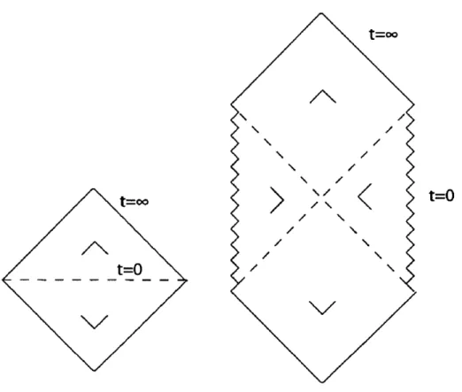
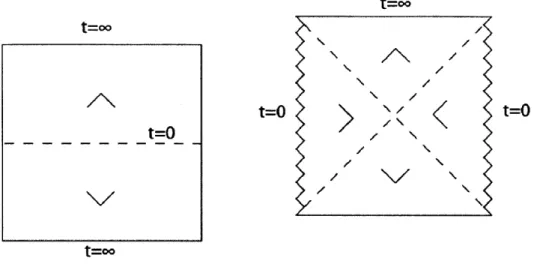
Schwarzschild-anti-de Sitter). For each of these cases, the conformal (or Penrose-Carter diagram) is presented; in these diagrams, each point corresponds to a two-hyperboloid. To provide more information about this suppressed two-hyperboloid, Bousso wedges are placed in each region of the diagram. These V-shaped wedges are visual aids that are constructed as follows: Intersect two null geodesics in the conformal diagram. Select the directions along these geodesics along which the factor multiplying the suppressed part of the geometry in the metric (in this case, s2 multiplying dH2) is decreasing. Draw the wedge

with the legs pointing in those directions. The wedge therefore points in the direction in which the suppressed geometry is expanding [7].

4.2.1 Hyperbolic Schwarzschild In the A = 0 case, the metric simplifies to

dt2

ds2 ₌

₊

_{± h(t)dx}2 _{+ t}2_dH!

h(t)

where 0 < t < o and -oo <cx < oo and

to

h(t) = 1l- .

The conformal diagram is shown in Figure 2. We see that

R.UV\O'~v'\' -t 60

so therefore there is a curvature singularity at t = 0 if to

#

0. We will

only need the future diamond of the hyperbolic Schwarzschild spacetime to construct the bubble collision spacetime geometries.

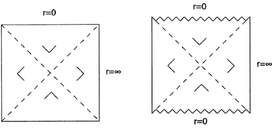
4.2.2 Hyperbolic Schwarzschild-de Sitter In the A > 0 case, the metric simplifies to

dt2

ds2 ₌

+ g(t)dx2 _{+ t}2 _dH2

g(t)

where 0 < t < oo and -oo < x < oo and

g(t) = 1 + 2 - _ 3 t

The conformal diagram is shown in Figure 3. We see that

8A2 _12t2

3 0

t=00 t=0

t=0

Figure 2: Conformal diagrams for Minkowski and hyperbolic Schwarzschild spacetimes (each point corresponds to a 2-hyperboloid)

t=oo

t=oo

t=o

t=oo

t=o

t=O

Figure 3: Conformal diagrams for dS and hyperbolic Schwarzschild dS space-times (each point corresponds to a 2-hyperboloid)

4.2.3 Hyperbolic Schwarzschild-anti de Sitter In the A > 0 case, the metric simplifies to

ds2 _=-f(r)dt2 _{+ dr}2 _+r2dH

2

f (r)

where 0< r< oo and -oo < t< oo and A

f

(r) = - r2_

3

ro

r

The conformal diagram is shown in Figure 4. We see that

R1OR1"A " 8A2

yx" ₃

12r2

r6

r=O r=O

>/

r=0o

Figure 4: Conformal diagrams for AdS and hyperbolic Schwarzschild AdS spacetimes (each point corresponds to a 2-hyperboloid)

4.3

Assumptions

We make the following assumptions in the treatment of bubble collisions that

follows:

" Domain wall - We assume that after two bubbles containing different vacuum states collide, a domain wall forms between them.

" Null shell of radiation - Null shells of radiation are emitted to satisfy energy-momentum conservation at the impact surface.

" Thin-wall approximation - We assume that domain walls and shells of radiation are sufficiently thin that they may be treated as membranes.

" Initially expanding - We assume that both bubbles are initially ex-panding after the quantum tunneling nucleation process is completed

and they begin semiclassical motion.

e Null Energy Condition

4.4

Kinematics of radiation shells and the domain wall

There will be a domain wall that separates the bubble spacetimes unless the bubbles were each in the same classical vacuum state.

5/

Figure 5: A spacetime diagram of a two-bubble collision in a frame in which the bubbles are nucleated simultaneously. The regions have the following properties (using the notation of the metric in Equation 4.1): (1) background metastable vacuum state (A > 0, so = 0), (2) left and (3) right bubbles

outside of the future lightcone of the collision (so = 0, A variable), (4) left and (5) right sides of the domain wall (so

#4

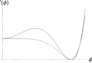
0 in general, A variable)

collision. For example in [17], the model used uses a complex scalar field in Minkowski space with the potential

V(#)

=

(k#|

2

₊

_a)(1#| 2 _-

_b)2

where a and b are real constants such that b > 2a (see Fig. 6). This potential has two local minima, one at

#

= 0 and the other at 1#| = b. A bubble is

formed when an instanton transition occurs between

#

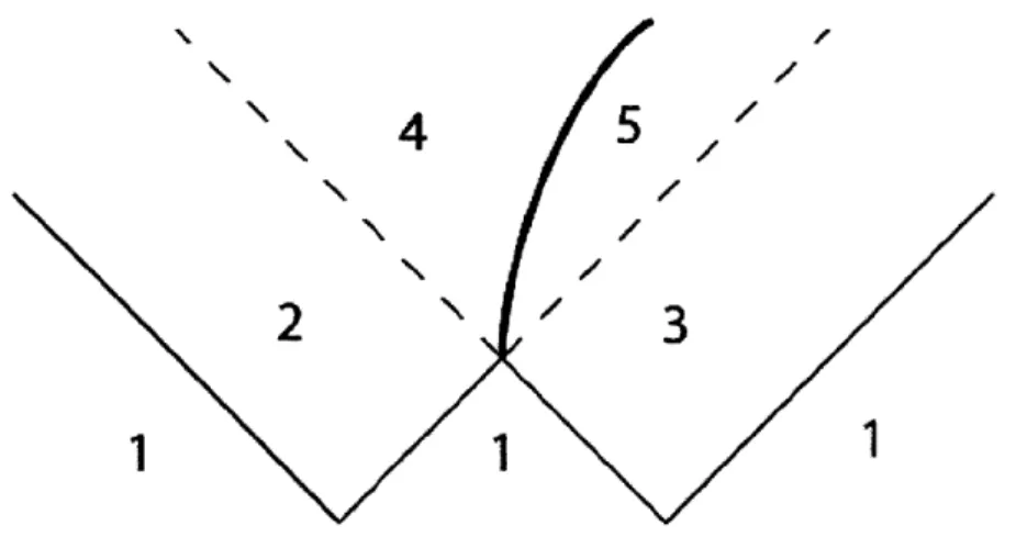
= 0 and 1#1 = b. No constraints are placed on the phase of the field in the second local minimum condition; we therefore expect that different bubble interiors will have field values with different phases. When these bubbles collide, null shells of scalar radiation will be emitted from the collision. These shells propagate as a kink in the phase of the field, interpolating between the original value of the phase and the average of the two phases. (If the phase difference is nearly r, the field will be nearly antisymmetric around the plane defined by points equidistant from the nucleation points of the two bubbles. No phase waves will form, and the resulting field configuration will remain antisymmetric.) Others report similar shells of radiation in different models of bubble collisions [1] [4} [13].

It seems plausible a priori that bubble collisions could generate primordial black holes. However, two-bubble collisions cannot create singularities, as shown in [20]. Due to the SO(2, 1) symmetry, two-bubble collisions also do not create large gravitational waves according to the hyperbolic analogue of the Birkhoff theorem.

At the point of collision of the domain walls of the two bubbles, there is an inertial reference frame (according to the equivalence principle). This is equivalent to saying that no conical singularities form at the point of collision. Consider the general collision of many sheets of matter or radiation shown

V(#I)

141

Figure 6: The shape of the double well potential considered in [17]

in Figure 7. Each (massive) sheet defines an inertial reference frame in which that sheet is at rest. The sheets of radiation can be treated by taking the limit as the velocity of massive sheets as the mass goes to zero. A boost from frame 1 to frame 2 is given by

(

cosh32,1

sinh

#2,1

A

2,1 -=

sinh32,1

cosh#2,1-The combination of two boosts results in a boost from frame 1 to frame 3:

A₃,1 =A3,2A2,1

cosh

#3,2

cosh#2,1

cosh#3,2sinh

#2,1

cosh(#

3

,

2

+ P2,1)

sinh(33,2 +132,1) + sinh#3,2 sinh 32,1 + sinh#3,2cosh32,1 sinh(#₃,2 +

#2,1)

cosh(#₃,2+

#2,1))

cosh#3,2 sinh

#2,1

+ sinh

#3,2

cosh

#2,1

coshp3,2cosh

#2,1+

sinhp3,2sinh

#2,1

_( cosh

#3,1

sinh

#3,1

sinh

#3,1

cosh

#3,1

n+m

n+1

fn+m,i

12

'n

Figure 7: Figure illustrating conservation of energy-momentum at a point of collision. Time flows upward. Each line represents a sheet of matter or radiation that is entering or exiting the collision point. The

#s

refer to the velocity of sheet one sheet in the reference frame of another sheet.

A boost from n to n

+

1 is

An+1,n

cosh -#n+1,n sinh -#n+1,n

sinh -#n+1,n cosh -#n+1,n

where

#n+1,n

> 0 since vn -vn+1 < 0

Since the composition of all the boosts must return to the original frame if the local spacetime is flat (that is, there is no conical singularity), we obtain the following condition:

n+m-1 n+m-1

A1,n+m Aj+1,j = 12 -4 1,n+m + E /j+1,j

0-j=1 j=1

4.5

Motion of domain walls

We will now solve for the motion of the domain walls in each of these prob-lems. To do this, we first derive the Israel junction conditions for treating surfaces in general relativity, then apply the needed conditions to domain walls in collisions between various types of bubbles (dS, AdS, Flat).

4.5.1 Israel junction conditions

We use the Gauss-Codazzi formalism to obtain the Israel junction conditions. We will use these conditions to determine the motion of the domain walls, denoted E, in the true and false vacuum regions. We will use Gaussian normal coordinates, where n indicates the direction normal to the domain wall. The metric in the Gaussian normal coordinates satisfies g" = gn= 1 and gni = 0. The extrinsic curvature is then given by Kij = -l'. Let

Sij =_ o-gij be the energy-momentum tensor on the surface E. We make

constant on E. The components of the Einstein tensor in these coordinates are

G - (3R _{+KijK'j- K2)}

G n - Ki m -0K=0

G - 3Gij -- On(K'j - & K) - KKj + 2 K2 + 2 JKabKa

where 3R, 3G , 0_{m refer to the values of the Ricci scalar, Einstein tensor}

components, and partial derivatives defined intrinsically on the

codimension-1 submanifold E [5].

Define

7yi mlim[Kij(n = +E) - Ki₂ (n = -E)],

~ 1

Kig j _{2 e-0O}- lim[Kig (n = +c) + Ki3 (n E)],

7 = 97gy, and K - g1'Kij, where the

+

and - labels denote the value of the extrinsic curvature on different sides of E. Note that

o

m 4-647)

=0.

We have (2) lim Gpdn = 87rSa e-40 4-fn (3) and / -~e

lim_ (&mKi" - O&K)dn = 0 e-40

E_

where E ± En' denotes evaluation on a surface moved slightly away from E in the normal direction. Integrating the Einstein tensor across E in the normal direction yields

_~~ 6Kbab)dfl

lim G'gdnlim im ]( 3 _{Gi - On(K'g - 6 K) - KK% + -o}

K2 _{+ -KK}

= -lim(K' j - 6K+ - K'_j - 6K_)

Combining this with Eq. 3, we find

7ij - gij7 = -8rSig.

This is called the first Israel junction condition.

Using junction condition and Eq. 2, we find that OmSim = 0, so am"o(agim)

0 and 6io = 0. Therefore o is constant on E. Contracting gab with the first

Israel junction condition, we obtain

gab" - ggab7 = 8,rogabg .

This implies that

= -127ra.

4.5.2 Flat

/

flat collisions

We present a detailed discussion of a possible simple collision scenario in the case of two Minkowski bubbles colliding in an inflating background de Sitter space. This will illustrate possible domain wall dynamics. We follow [9] in this section, filling in details in the calculation at many points.

We assume that the domain walls of the two bubbles suffer an elastic collision and therefore bounce off of each other. There may be excess energy that is emitted in a null shell of scalar radiation.

We start by considering the metrics for the false vacuum region of space-time (A > 0 and m+ = 0), the true vacuum inside of the bubbles (A = 0 and

m- z 0 in general), and the region beyond the null shells in false vacuum (A > 0 and m+ / 0): ds2 d2 =

-

2 + f (s)dx2

₊

_s2_dH22 where s2A 2m+ 3 S

f_(s)

=1 2m_ We note Gn+ - Gn- = -A, so 3R+ KaKa _ K2)+ (3R+ KabK - K) -- A.

This conveniently eliminates the 3_{R. Therefore,}

(KaK"? - Kc-K"') - (K2 - K2) = 2A. (4)

Contracting Kab with the first Israel junction condition, we find

kabgab(8eo-) -

k

abg 1.

Evaluating each of the terms in this equation gives

ab -1

Kab = (K±bKb+ KaK_

kcngaby

= (K+ + K-)(K+ - K-) = (K2 - K2).

2 2 +

Combining this with Eq. 4, we find

Kbgab A (5)

87ro-We will now use these equations to calculate the motion of the domain walls. We parametrize the domain wall motion by sa =.ta(r) and s = s(r),

where

s

k and ± denotes the x position as seen from the two different regions of spacetime. The vector tangent to the domain wall is

u" a + = (Y1,7 0, 0,

dr

and the normal vector is

n=i = (-A, 0, 0, Y+),

where

We will now begin to suppress the i sub- and superscripts for notational clarity (except where

+

or - is specifically intended). Note

Ua na

na"

fY

2_{_-1A}2 =-=f-Y b _ fy2I

nc" = 0

Taking the covariant derivative of this first equation gives

D -(uau")_dT Duo 2ua D - 0, d-r which implies D2xr DuO ndT *d-r D2x -8-dr2

A

D2_S f 2Y d-2 D2s 1 D2_S

fY

dr2

The geodesic equation gives

D2s

.= § + r, upu 88 XX*

(6)

Since asss df -1 gx df ds ds and 1 f df-' 1 df S* -g*? .g., * 2 2 ds 2fds 1"8 f df 2 _xx 2 ds we have 1 df A2F, y+ Y2r _{: 2 ds} so therefore D 2s 1 df T-2 -S2 s

Let A = A'e; be an arbitrary vector in E. Then

OA s -= (A's-,i)=2*VjA"+A .. Note that i -Ki since n -

-K--and Il| 1. Thus

O A

= iVj A" - Ai Kijn' and

u'- = eiu'Vjut - utuKii.

The first term is zero because u is a geodesic on E. Therefore

DuoK

= - U.7

Kiin

From this, we have so Dua na dr~_ = -uZUn7Ki, J I 1df -u _* 2ds. Adding the + and - equations gives

f..i1

df+\

2 ds2d)

1 1 df_

-2uujiKj-yij = 8-rogij + ygij -47ro g

duyig = 47roddgig =

-47ro-Subtracting the + and - versions of Eq. 7 gives

1 df_ -47ra. 2 ds

1 .. 1

df+)

f+

Y+ 2 ds ) 1 ..

fY_

S

We now compute the entries of the extrinsic curvature in the above metric:

S= - =Ongij

Koo -Ongoo 1 _{= -Ons2}1

2 2

1

Ko =

Ongk

= 9(Ons) sinh2 _{+ s}2 _{sinh 08, sinh 0 = A(Ons) sinh}2 ₉ 2

Ko. = 1nge = 0 2

Since Ons = s n' = g"n, fY (up to sign), we have Koo = sfY=s 2

-f

Koo= sfsinh2_0Y=ssinh2₀ 2

_--

_{_f.}

(7) 1 Note that 1

(.

fY S

(9-Therefore

oog -- M -(f+Y+ + f-Y-)

2s

and

Ua Ubkab -Kab(g ab -9 gaD gbO -9 ₉aO 9 k)

1 = abg

+

-(f y + fY) S A 1 = _{+ - (f+Y+ + f-Y-).} 87w- s We finally obtain 1 1df+ 1 1 df ) 2 2 A - S - -

+

+

- A2 - f+- A2 _A

f+

Y+

2 ds

f-Y_

2 ds

s

s

4,ro-This is the equation of motion of the domain wall in terms of s(r). We will now simplify it and solve it in cases of interest.

Define Za - 52 - -fLY± (up to sign) and c 27r-. Then

Z, A 1 df 1 2 A - (Z;+ +

Z-_)

+ -(Z+ + Z-) =A-s s 2c' and (Z+ - Z_) = -2cs. (8)

Define U Z+

+

Z_ and V Z+ - Z. Then we have

U+2 A

s s 2c

and

which implies that V -2cs + const. The solution for U is 1 U = (f+ - f-) 2cs sA m+ - m_ 6c 2cs2 -A A (m-m) 6c sac

since it is clear that

sAA

s#+2AU= .

2c

Since Za = !(U i V), we finally have

2f

-fLY = -Zi±= - + f- sc. (9)

4sc

We examine this equation in three cases of interest:

CASE 0: A=O andm+=O

This case is the case of flat space in all regions of spacetime. In flat space, we have

f+

= f = 1 and Y+ = VTT2-1. Eq. 9 then simplifies to

2§ + 4_A_4 2 - 1 _ A 2C4

V87---l S 47ro- a

where A = 87rEd

(E

is the vacuum energy associated with the cosmological constant A). We have

.1 s = %/1 -2 and As2 - =(10) We have defined ,sd

so x = 'A. Differentiating Eq. 10, we obtain s xs=x=

(1 - z)3/2 (I ±1 )2' so

-2)3/2 +

Rearranging this equation gives

o-ss"= -20-'(1 - I2) + sC4(1 - 2)3/2

This agrees with [17] (after taking the opposite sign of ', which is irrelevant

because the problem is symmetric around z= 0).

CASE 1: Af0,m+=0

This case describes expansion of bubbles before collision. Before collision, we expect the solution for the bubble walls to be physically identical to the solution obtained by assuming SO(3,1) symmetry (that is, the solution presented in [10]) because the two bubbles are not yet in contact with each other. Eq. 9 implies

(A -s

247ro- +27r

R

where

R=

27ro2 _{+ A/24r}

This is the same type of accelerating domain wall behavior presented in [10]. Therefore the general solution holds in two important special cases.

CASE 2: A0,m_=0,m+o

This case describes expansion of bubbles after the collision when no null shells are emitted. Since m_ 0, we have

f_

= 1. From Eq. 9, we have

- I1(S2 A 2m+

fkz=

A2 _-1=2ros+ Vs _{87rs 3 s} and s2A 2m+ _(s 2 A 2m+) f~i+= i 2 - - - -2-7rus + 3 s 8ros 3 s 1+

We posit that, as measured in de Sitter space, the incoming domain wall velocity equals the outgoing velocity in subsequent collisions (which occur

whenever 2 0):

This allows us to numerically integrate the equations of motion to compute the motion of the domain walls (see Figure 8).

4.5.3 Motion of the domain wall for general collisions

For the general case, we suppose that only one domain wall is results from the collision and the rest of the energy is expelled in the null radiation shells, as in Figure 5. We summarize and quote results from [3] and {7].

On the domain wall we assume an energy-momentum tensor of the sim-plest form, leading to:

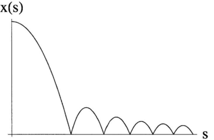
X(S)

S

Figure 8: Motion of the domain wall separating two Minkowski bubbles after a collision (in a flat background, for simplicity)

The metric must be continuous across the domain wall according to the junction conditions, so the induced metric is

ds 2w = -dr 2

+

R2_(T)dH22

where R(r) = t(r) or r(r) from our previously discussed metrics. The Israel junction conditions imply

(L R2 JL() -CR R2 + JR() = oR

analogous to Equation 4.5.2, where

C

t1 and J = -h(t) or -g(t) or f(r).

Solving for

N

2

,

we obtain

1 2 - V () [JL(R) - JR(R) - o.2R2]2

R

2 _V

_{5(R) =}

_{JR(R)+ 4o}2_R2

which reduces the problem of the domain wall motion to that of a particle in a potential. We will now state the solution of this problem for various values of the cosmological constants on either side of the domain wall.

dS

/

AdS or flat

/

AdS: For collisions between AdS and dS or flat

bub-bles, we have

2 + F

/h2

- g=o-R.

For large R, this simplifies to

2

_R2

with

2 __Aas/at 1 (,2_ AAds + AdS/flat )2

A- 3 +4o-2 ₃

Using this in the junction condition gives

1 2 + AAdS AdS/flat 1 1 2 _ AAds + AdS/flat _

2o 3 20 3

We consider the following options in general for the tension a-:

* Tension greater than AdS scale - Domain wall accelerates away from dS/flat bubble (see potential in Figure 9).

" Tension equal to AdS scale - Domain wall coasts and does not accelerate (see potential in Figure 10).

* Tension less than AdS scale - Domain wall accelerates towards the dS/flat bubble. In flat / AdS collisions, this condition is im-possible if the BPS bound is not violated (which will be true if supersymmetry is assumed) [3]. In dS

/

AdS collisions, the dS

bubble is not destroyed because the domain wall can only move through part of the total expanding spacetime.

dS

/

flat: In dS

/

flat collisions, we find through similar calculations to the previous case that the domain wall accelerates away from the

V(R)

Figure 9: Form of the effective potential governing the motion of the domain wall in the non-extremal case

V(R)

R

Figure 10: Form of the effective potential governing the motion of the domain wall in the BPS case

Minkowski bubble. Minkowski bubbles are therefore always safe from such collisions.

dS

/

dS: In a collision between two de Sitter bubbles with cosmological

con-stants AL and AR, the domain wall will accelerate towards the bubble with higher cosmological constant (suppose AL > AR). This may pro-vide an anthropic argument for a low cosmological constant if collisions are sufficiently frequent [7].

We see that observers living in bubbles with small positive cosmological constant are safe from most types of collisions.

4.5.4 Note on Raychaudhuri's Equation

In [3] and [7] it is claimed that the Null Energy Condition and the Ray-chauduri equation imply that "along radially directed null lines where the

H2 is decreasing it must shrink to zero size." We show this here.

The Raychaudhuri equation for a congruence of null geodesics kA is

dO

₌ 62 2 _k _ -- _{- Rpk~k" v} cIA 2 , where or2 ₌ W- 2 = oV/, o, 6 - 1h,, hhVka,

O6V h'hPV(pkA), and hAV = gjV - kykV.

Using Einstein's equation, we see that

Rk~k" = 8,r(T,, - 1gT kk"

= 87rT, kIkv.

If the Null Energy Condition holds, then T,,k" k" > 0, so

dO 02

-K---dA 2'

since o2 > 0. Since 9 = Vtki' - -2/s, we have

ds

dA

-Therefore if s (the factor controlling the size of the 2-hyperboloid) is decreas-ing along a null geodesic, it continues to decrease to zero.

5

The view from inside

We will examine the trajectories of the null shells of scalar radiation and (asymptotically) the accelerating domain walls as they are seen from the bubble interior.

5.1

Null shells in flat background and interior

We employ three metrics for the same flat spacetime in order to determine the equation of motion for the null shells.

Flat SO(2, 1):

-ds

2 _{+ dx'}2 _{+ s}2_(dp2 _{+ sinh}2 _pd#2₎

This metric is most convenient for describing the bubble collision in the collision frame.

Flat SO(3, 1): -dt 2 + dx2 _{+ dy}2 _{+ dz}2

This is the standard metric for Minkowski space. FRW in open slicing: -dr 2 _{+ r}2

(d 2 _{+ sinh}2 _((d9 2 _{+ sin}2 _9d#2₎₎

open slicing. We will center it on one of the bubbles, so the coordinates are off-center in the above SO(2, 1) coordinates by a distance b in the x direction. The way to convert between the coordinates corresponding to the above metrics is as follows:

s cosh p = t =T rcosh (

x'+ b = x = Tsinh ( cos 0

s sinh p sin

#=

s sinh p cos

y =-rsinh sin 0 sin#

z = T sinh sin 0 cos#.

From these equations, we obtain the following:

T2 s2 -(x

+

b) 2 / 2 tanh2 8

+ tanh

2 s2 tan2 6 sinh2 p. x/2

The motion of the null shell is a simple linear equation in the SO(2, 1) coor-dinates: x' = s - 2b. This yields the following equations:

((r, p)

tan2

O(,T, P)

tanh-1

₍

₂

_+b

2

+

tanh2P]

T 2 - b2 b sinh 2 to

Eliminating p, we obtain the following relationship between (, T, and 0:

(

T2 -b2 _20~ T2-b tan 6 1 +2 b2tan20 72- b2 T2 _{+ b2)} ((r 0) =

tan-(-)

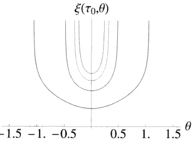
Figure 11: Sketch of null shell radius dependence on T as seen from inside

the bubble for 0 = 0 in a flat background and bubble interior.

(o,0)

-1.5 -1. -0.5

0.5

1. 1.50

Figure 12: Sketch of null shell radius dependence on 0 as seen from inside the bubble for varying T (T is smallest for the blue curve and increases on higher curves) in a flat background and bubble interior.

5.2

Null radiation shell in de Sitter bubbles

We will consider the motion of the null shells in the limit where to

<

tc,

where tc is the coordinate at which the collision occurred. This implies that to good approximation we can treat the spacetime on both sides of the null shell as flat. We will employ two metrics in this section as we used them in the previous section:

de Sitter SO(2, 1) metric:

de - dt2 t2 d2 2(P 2

2

= -

+2$1

+

- dx2

+

t2(dp2

+ sinh

2 pd$2)

1 + t2/1i2 ₁₂₎

where x ~ x

+7rl,

0

<

p < oo, 0 < 0 < 27r. (We will from here on use units

for t such that 1 = 1.)

de Sitter FRW metric in open slicing:

df2 = -dr 2 _{+ sinh}2 _(d 2 _{+ sinh}2 _(d92 _sin2 _2d02))

where 0

<

< oo, -7r < 0 < 7r.

The equations connecting the two different sets of coordinates are [8] cosh T = v1

+t2

cos x

sinh T sinh( cos 0 = V1 +t2sin x

sinh r cosh& = t cosh p sinh T sinh C sin 0 = t sinh p.

It is clear from the above metric that null geodesics in SO(2, 1) obey

dx 1

dt 1+t 2_'

so

for some constant of integration d. Let xo = 2 tan-1 d.

We have

tan x = tanh r sinh (cos 0 and

t2 = sinh2 r(cosh2 _sinh2 _0sin2)

so

tan-'[tanh r sinh cos

0]

= tan-'[sinh r cosh2( - sinh2 ( sin2 0] + mo.

ForTr -+0 and 0 0, tan-'(sinh() tan-'(-jle cosh()

+ xo,

where we have taken the negative square root of cosh2 _{. The value of ( at 0 = 0}

as T -+ o is

((T -+ oo, 0 = 0) = sinh-1 .

This is the expected behavior of null geodesics in de Sitter space: They asymptotically approach a finite coordinate distance from any given point.

6

Observational Signatures

The SO(2,1) symmetry implies that if we could observe the effects of a bubble collision, we would see them affecting a region contained inside of a disk in the CMB, since the intersection of the future lightcone of the colliding bubble, the past lightcone of an observer, and the surface of last scattering is a disk. It is unclear what we should expect to see inside of this disk, but the boundary of the disk may be a sharp boundary, defined by the maximum causal influence of the collision. Photons may be reflected by the receding domain wall between the bubbles. They would receive a red- or blue-shift

from this encounter. Another signal is that pure E-mode polarization is expected to be generated from the collision, centered around the collision

[11].

7

Conclusions

7.1

Status of Observations

One group has recently presented results of an analysis that identified four candidate collision sites in WMAP data [12]. Data from the Planck satellite, especially polarization data, will be helpful in confirming these candidates or eliminating them.

Bubble collisions may have observable effects on large-scale structure. High-redshift galaxy surveys may provide evidence for bubble collisions that could be corroborated with evidence in the CMB.

7.2

Future Directions

One goal is to calculate the modified primordial density perturbation from the collision of two bubbles in the same classical vacuum. This is the simplest possible collision scenario. No domain wall would form, and only the null shells and slight deviations from isotropy would be detectable in the primor-dial density perturbation. This may yield a model-independent prediction of the modifications to the fluctuations that we expect to see inside of the aforementioned disks on the sky.

uni-verse, this will provide direct confirmation of eternal inflation and may pro-vide information about the existence and nature of the string theory land-scape. However, if collisions are not detected, it may be possible to use this information to constrain pictures of eternal inflation or the landscape. Such inferences may rely upon choosing an appropriate measure for calculating probabilities of events in the multiverse (a challenging problem), so there may be much work remaining on this approach.

References

[1] A. Aguirre, M. C. Johnson, and M. Tysanner. Surviving the crash:

assessing the aftermath of cosmic bubble collisions. Phys. Rev. D,

79(12):123514, 2009.

[2] Andreas Albrecht and Paul J. Steinhardt. Cosmology for grand unified theories with radiatively induced symmetry breaking. Phys. Rev. Lett.,

48(17):1220-1223, Apr 1982.

[3] S. Shenker B. Freivogel, G. Horowitz. Colliding with a crunching bubble.

Phys. Rev. D, 21:3305-3315, 1980.

[4] Jose J. Blanco-Pillado, Martin Bucher, Sima Ghassemi, and Frederic Glanois. When do colliding bubbles produce an expanding universe?

Phys. Rev. D, 69(10):103515, May 2004.

[5] S. K. Blau, E. I. Guendelman, and A. H. Guth. Dynamics of

[6] Raphael Bousso and Joseph Polchinski. Quantization of four-form fluxes

and dynamical neutralization of the cosmological constant. JHEP,

06:006, 2000.

[7] S. Chang, M. Kleban, and T. S. Levi.

Astropart. Phys., 2008(4):034, 2008.

[8] S. Chang, M. Kleban, and T. S. Levi.

on the cmb from cosmological bubble

Phys., 2009(4):025, 2009.

[9] W. Z. Chao. Gravitational effects in 28(8):1898-1906, 1983.

When worlds collide. J. Cosmol.

Watching worlds collide: effects collisions. J. Cosmol. Astropart.

bubble collisions. Phys. Rev. D,

[10] S. Coleman and F. de Luccia. Gravitational effects on and of vacuum

decay. Phys. Rev. D, 21:3305-3315, 1980.

[11] Bartomiej Czech, Matthew Kleban, Klaus Larjo, Thomas S. Levi, and

Kris Sigurdson. Polarizing bubble collisions. Journal of Cosmology and

Astroparticle Physics, 2010(12):023, 2010.

[12] Stephen M. Feeney, Matthew C. Johnson, Daniel J. Mortlock, and Hi-ranya V. Peiris. First observational tests of eternal inflation, 2010.

[13] John T. Giblin, Lam Hui, Eugene A. Lim, and I-Sheng Yang. How to

run through walls: Dynamics of bubble and soliton collisions. Phys.

Rev. D, 82(4):045019, Aug 2010.

[14] Alan H. Guth. Inflationary universe: A possible solution to the horizon and flatness problems. Phys. Rev. D, 23(2):347-356, Jan 1981.

[15] Alan H. Guth. Eternal inflation and its implications. J. Phys., A40:6811-6826, 2007.

[16] Alan H. Guth and Erick J. Weinberg. Could the universe have recovered

from a slow first-order phase transition? Nuclear Physics B, 212(2):321

- 364, 1983.

[17] S. Hawking, I. G. Moss, and J. M. Stewart. Bubble collisions in the very

early universe. Phys. Rev. D, 26(10):2681-2693, 1982.

[18] Andrew R. Liddle and David H. Lyth. The Primordial Density

Pertur-bation: Cosmology, Inflation and the Origin of Structure. Cambridge

University Press, first edition, 2009.

[19] Andrei D. Linde. A New Inflationary Universe Scenario: A Possible

Solution of the Horizon, Flatness, Homogeneity, Isotropy and Primordial Monopole Problems. Phys. Lett. B, 108:389-393, 1982.

[20] I. G. Moss. Singularity formation from colliding bubbles. Phys. Rev. D,

50(2):676-681, 1994.

[21] Steven Weinberg. The cosmological constant problem. Rev. Mod. Phys.,

61(1):1-23, Jan 1989.

[22] Steven Weinberg. Cosmology. Oxford University Press, first edition,