Co-simulation of algebraically coupled dynamic subsystems

Co-Simulation of Algebraically Coupled Dynamic Subsystems

by

Bei Gu

B.S., Mechanical Engineering Shanghai Jiao Tong University, 1992

M.S., Mechanical Engineering Arizona State University, 1997

Submitted to the Department of Mechanical Engineering in Partial Fulfillment of the Requirements for the Degree of

DOCTOR OF PHILOSOPHY at the

MASSACHUSETTS INSTITUTE OF TECHNOLOGY September 2001

© 2001 Massachusetts Institute of Technology All rights reserved

Signature of Author_ Certified by Accepted by MASSACHUSETTS INSTITUTW OF TECHNOLOGY

DEC 1 0 2001

BARKER

August 25, 2001

H. Harry Asada, Ford Professor of M/chanical Engineering Thesis Supervisor

Ain A. Sonin Chairman, Department Graduate Committee

Co-Simulation of Algebraically Coupled Dynamic Subsystems

By Bei Gu

Submitted to the Department of Mechanical Engineering on August 24, 2001 in Partial Fulfillment of the Requirements for the Degree of Doctor of Philosophy in

Mechanical Engineering ABSTRACT

In the manufacturing industry out-sourcing/integration is becoming an important business pattern (not a clear statement-integration still done in house--component design and manufacturing outsourced). An engineering system often consists of many subsystems supplied by different companies. Bridge between thoughts is weak. Object-oriented modeling is an effective tool for modeling of complex coupled systems. However, subsystem models have to be assembled and compiled before they can produce simulation results for the coupled system. Compiling models into simulations? is time consuming and often requires a profound understanding of the models. Also, the subsystem makers cannot preserve their proprietary information in the compilation process. This research is intended to address this problem by extending object-oriented modeling to object-oriented simulation called co-simulation. Co-Simulation is an environment in which we can simultaneously run multiple independent compiled simulators to simulate a large coupled system.

This research studies a major challenge of object-oriented simulation: incompatible boundary conditions between subsystem simulators caused by causal conflicts. The incompatible boundary condition is treated as an algebraic constraint. The high index of the algebraic constraint is reduced by defining a sliding manifold, which is enforced by a time sliding mode controller. The discrete-time approach fits well with the numerical simulation since it can guarantee numerical stability. A Boundary Condition Coordinator (BCC), which implements the discrete-time controller, makes the incompatible boundary condition compatible. Multi-rate sliding controllers are developed to guarantee the stability of the sliding manifold with any integration step size for the subsystem simulators. A multi-rate sliding mode scheme is specially devised to minimize information disclosure from the subsystem simulators and to facilitate pure numerical computation. The influence of the BCCs on the rest of the subsystem simulators is studied using the input-output linearization theory.

The Co-Simulation software environment is developed in Java. Subsystem simulators and BCCs run as independent processes in the Co-Simulation environment. Class templates containing all necessary functions for different types of subsystems are defined. Engineers can easily build a subsystem simulator by simply providing only the mathematical model, which will be hidden after the subsystem simulator is made. Integration engineers can assemble subsystem simulators into simulation of the large coupled system by merely making connections among subsystems. The object-oriented class design makes it possible to extend the Co-Simulation over the Internet or to compile subsystems into a single thread simulator.

Thesis Supervisor: H. Harry Asada

Acknowledgements

I would like to express my sincere gratitude to my advisor, Professor H. Harry Asada, for his intellectual guidance, constant encouragement, and wide-ranging support. I would like to thank my committee members, Professors Kamal Youcef-Toumi and David R. Wallace, for their

inspiring advice, and Dr. Sheng Liu for his invaluable guidance.

Our group is always a fun and dynamic place. I will remember Booho, Brandon, Carolyn, Danielle, Peter, Phil, Steve, Xiangdong, Yi, Yong and other members of the d'Arbeloff Laboratory for Information Systems and Technology for their help and friendship.

My family has been a great source of love and encouragement. My having the opportunity to write this thesis results from what I have learned from my parents. Most of all, thanks to my wife Stephanie. I will not be able to finish my research project without Stephanie's support.

Finally, I wish to thank my sponsors Daikin Industries, Home Automation and Healthcare Consortium, and Matsushita Electric Industrial Company.

Table of Contents

I

1.1 M otivation ... 9

1.2 Thesis contribution... 10

1.3 Thesis organization ... 12

II Incom patible Boundary Condition... 15

2.1 M odeling of Subsystem s... 15

2.2 Algebraic Constraints... 17

2.3 Differential Algebraic Equation and Index Reduction... 19

2.4 Resolving of Algebraic Constraints ... 20

2.5 Pure Discrete-Tim e Boundary Condition Coordinator ... 23

III Discrete-Tim e Sliding M ode... 26

3.1 Introduction to Discrete-Time Sliding M ode Control... 26

3.2 Single-Rate DTSM ... 27

3.2.1 Dynamics of the Sliding Function... 27

3.2.2 Continuous Control Input... 28

3.2.3 The Invariant Set around the Origin... 29

3.2.4 Proof of Convergence... 30

3.3 The M ulti-Rate DTSM ... 33

3.3.1 Two-Tim e Scale Problem ... 33

3.3.2 Im plem entation of DTSM ... 34

3.4 The Accuracy of the Original Algebraic Constraint ... 37

3.5 Exam ple... 38

3.5.1 M odel ... 38

3.5.2 Results ... 40

3.6 Extension to M ultiple Subsystem s ... 43

IV Input-Output Linearization Analysis of Co-Sim ulation... 47

4.1 The Effect of ... 47

4.1.1 Exam ple... 47

4.1.2 A Linear Case... 51

4.2 Influence of DTSM on Stability of Subsystem s...53

4.2.1 Subsystem s in Partial Controller Canonical Form ... 54

4.2.2 General Nonlinear Subsystem s ... 58

4.3 Subsystem Relative Order and the Index of DAE...59

V Co-Sim ulation with M inimum Inform ation Disclosure ... 60

5.1 Hybrid Implementation of Boundary Condition Coordinator...60

5.2 Disadvantages of Hybrid Implem entation... 63

5.3 Constructing Pure Numerical DTSM Using Minimum Information ... 64

5.4 Decoupled M ulti-Rate DTSM ... 67

5.4.1 Integration path ... 67

5.4.2 Convergence in a Sm all Tim e Scale ... 69

5.4.3 Convergence in a Large Tim e Scale ... 71

5.4.4 Num erical Examples ... 72

VI Softw are D evelopm ent... 77

6.1 Softw are for D ifferent Functional Requirem ents... 77

6.1.1 Co-Sim ulation Running on One Com puter... 77

6.1.2 Co-Sim ulation Running over The Internet... 78

6.1.3 Single-Thread Sim ulation ... 79

6.2 Softw are Architecture ... 80

6.3 Object-Oriented D esign of Subsystem Sim ulators...82

6.3.1 Object-Oriented Design... 82

6.3.2 Synchronization... 83

6.3.3 Com putational Logic... 85

6.3.4 Class Tree...88

6.4 U ser-friendly System Integrator D esign ... 91

VII Co-Sim ulation of a H VAC System ... 94

7.1 Introduction of Building Energy System ... 94

7.2 Modeling of Multi-unit Air-Conditioning/Heat Pump System... 96

7.2.1 Tw o-N ode H eat Exchangers ... 96

7.2.2 A ccum ulator ... 97

7.2.3 Com pressor... 97

7.2.4 Expansion V alve ... 98

7.3 Co-Sim ulation Setup ... 99

7.3.1 Subsystem Sim ulator Coding ... 99

7.3.2 System integration... 101

7.4 Results ... 102

VIII Conclusions and D irections for Future W ork ... 106

List of Figures and Tables

Figure 2.1.1 Bondgraph model of a subsystem ... 16

Figure 2.2.1 Co-Simulation of dynamic subsystems with different boundary conditions...17

Figure 2.2.2 Incompatible boundary condition caused by numerical difficulty... 18

Figure 2.4.1 A lgebraic constraint... 21

Figure 2.4.2 Algebraic constraint eliminated...21

Figure 2.4.3. Fictitious spring and damper... 22

Figure 2.4.4. Modeling the solution of DAE as a control system ... 23

Figure 2.5.5. Boundary Condition Coordinator resolves incompatible boundary condition...25

Figure 3.1.1 Pseudo sliding mode in the discrete-time domain. ... 26

Figure 3.1.2 Sliding mode in the continuous-time domain ... 27

Figure 3.2.1 Illustration of the equivalent control, minimum control magnitude and control input. ... 3 1 Figure 2.2.2 Phase portrait of the discrete-time sliding mode motion. ... 33

Figure 3.3.1 Possible implementations of the multi-rate algorithm... 35

Figure 3.4.1. s - g relation viewed as linear filters. ... 37

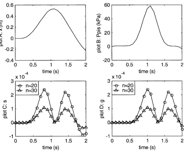
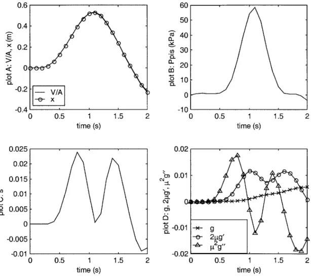
Figure 3.5.1 Coupled hydraulic and mechanical systems... 39

Figure 3.5.2 Causal conflict between two subsystems... 39

Figure 3.5.3 Results of the inconsistent initial condition... 41

Figure 3.5.4 Results of consistent initial condition... 42

Figure 3.6.1 A common effort junction with compatible boundary conditions... 44

Figure 3.6.2 A common effort junction without a subsystem dictating the effort variable...44

Figure 3.6.3 A common effort junction with multiple subsystems providing the effort variables. ... 4 4 Figure 4.1.1. Effects of parameter/p (u = 1). ... 48

Figure 4.1.2. Effect of parameter u (u= 0.1)... 49

Figure 4.1.3 Effect of parameter u (u = 0.04)... 50

Figure 4.1.4 The block diagram of a linear system... 51

Figure 4.1.5 Effect of p in a linear system ... 52

Figure 4.2.1 Block diagram view of realization of algebraically coupled systems. ... 53

Figure 4.2.2 Block diagram of Input-Output linearization control. ... 54

Figure 4.2.3 Example of systems in partial controller canonical form. ... 55

Figure 5.1.1. Hybrid implementation of the Co-Simulation. ... 61

Table 5.1.1 Computational sequence of the Co-Simulation...62

Figure 5.4.1 Different ways of enforcing the sliding function... 66

Figure 5.4.2 Schematic of the decoupled multi-rate DTSM. ... 68

Figure 5.4.3. Boundary variable for different vo. ... 73

Figure 5.4.4. Sliding variable for different vo. ... 74

Figure 5.4.5. Sliding variable for different n-vo. ... . . . .. . . . 74

Figure 5.4.6. Boundary variable for different n-vo. ... . . . .. . . .75

Table 5.5.1. Communication among subsystem simulators and BCC...76

Figure 6.1.1 Structure of Co-Sim ulation... 78

Figure 6.1.2 Structure of the Internet-based Co-Simulation ... 80

Figure 6.3.2 Mulit-thread input/output of subsystems ... 85

Table 6.3.1 Subsystem characteristics...86

Figure 6.3.3 Common computational logic...86

Figure 6.3.4 Subsystem simulator logic of causal dynamic systems. ... 87

Figure 6.3.5 Subsystem simulator logic of BCCs...88

Figure 6.3.6 Subsystem simulator logic of pure algebraic systems. ... 88

Figure 6.3.7 Subsystem simulator logic of source systems. ... 88

Figure 6.4.1 System integration environment...91

Figure 3.6.8 Class tree of subsystem simulators. ... 93

Figure 7.1.1 A commercial building HVAC system (courtesy Daikin)...95

Figure 7.2.1 The two-indoor-unit air-conditioning/heat pump system ... 97

Figure 7.3.1 BCCs connecting the indoor units and the accumulator... 100

Figure 7.4.1 Plot of sliding function s... 103

Figure 7.4.2 Plot of m ass flow rate h, . ... ... 103

Figure 7.4.3 Plot of Pressure P ... 104

Figure 7.4.4 Plot of Mean void fraction Y... 104

Figure 7.4.5 Plot of tube wall temperature T ... 105

I

Introduction

1.1

Motivation

People have developed many modeling and simulation technologies for different purposes over the years [Sinha et al, 2001]. System modeling is an important tool used by engineers for studying and designing engineering systems. Simulation then makes it possible for engineers to test the engineering system in the virtual realm before building the hardware. Modeling and simulation are closely related. The model serves as the basis for the simulation while simulation computes the prediction of the model. Modeling and simulation reduce both the time and the cost associated with the product development.

Object-oriented modeling approaches were first introduced in the late 1970s to deal with complex and multi-disciplinary systems [Otter and Cellier, 1996]. Among many object-oriented properties, modularity is the most important. Reusable subsystem models, which are developed by various experts, can be assembled to represent different large system models. The typical procedure of simulation is as follows: modeling of subsystems, assembling subsystem models, compiling the overall system model and solving of compiled system model.

Use of simulators is not only a powerful engineering methodology for design and analysis but also an important tool with which engineers communicate to each other. In addition to traditional specifications and data sheets, engineers now communicate by exchanging simulators representing the whole behavior of the components and systems they develop. In the automobile industry, for example, carmakers request that suppliers provide simulators of supply parts, and evaluate them by connecting the supply part simulators to the engine simulator and body simulator of the automobile. In turn, carmakers provide the suppliers with simulators depicting the conditions of the automobile system so that the supplier can develop the right parts to meet the specifications. Today's carmakers can communicate with thousands of suppliers through a supply chain management system over the Internet. In the air conditioner industry, former competitors are now forming an alliance to use common components and integrate their products. Simulators representing detailed behavior of individual units are exchanged to streamline communications among engineers of alliance partners and complete thorough engineering analysis and product development in a limited time.

" It requires engineers to go through all of the compilation and solution procedure before the

simulation results of the coupled system can be obtained;

" Some component makers may want to keep their intellectual property private, yet providing models of their components exposed many details of their design;

0 Different components of a coupled system may require quite different solution methods which may further complicate the process of converting models to simulations.

Extending the concept of modularity a step further, i.e., using objects of subsystem simulators instead of objects of subsystem models, a new simulation environment is proposed. Termed as Co-Simulation, it is software environment for simultaneously running a collection of subsystem simulators. When subsystem simulators are connected, simulators will produce the simulation result of the large system without going through the complex procedure of compilation and of numerical solution. Subsystem component simulators coded by different suppliers will interact with each other using predefined inputs and outputs. Simulators can then work together if they have compatible inputs and outputs. The internal implementation of the simulators is solely decided by their designers. The system integrator only needs to know the interface of the subsystem simulators. Therefore, the aforementioned three drawbacks of the object-oriented modeling can be eliminated.

The proposed object-oriented simulation technology will be an essential tool to facilitate upstream and downstream cooperation along the supply chain. The downstream companies will be able to test the integrated system with component simulators supplied by the upstream companies. The component makers also will test their products to find how their components work with other components by running simulators of all of the components together. In this way, engineers from the entire supply chain can communicate by co-running their subsystem simulators. Ultimately, simulators become the modern specification sheets for any component, but with a much richer array of available information.

1.2

Thesis contribution

Unlike object-oriented modeling, which uses a declarative approach to describe the dynamic system, a simulation must use a procedural approach to obtain the numerical results. The procedural approach defines the relation between dependent variables and independent variables through assignments. Assignments are basically causal definitions. The declarative approach

defines the relationships between variables by using equations without causal information. Simulators are basically numerical solvers for certain models. Numerical algorithms are then usually realized by procedural computer programs. Therefore, when simulators are assembled to represent a large coupled system, causal conflicts may occur due to the fixed causal assignments. Causal conflict is therefore the major challenge of the object-oriented simulation.

An incompatible boundary condition resulting from the causal conflict is modeled as an algebraic constraint. The coupled system is considered to be a control problem and the algebraic constraint is treated as the desired trajectory. Thus the system described by the high index Differential Algebraic Equation (DAE) becomes a high relative-order feedback control system. A sliding manifold is used to reduce the high relative order. Since the simulators are discrete-time systems, a discrete-discrete-time sliding mode controller is used to enforce the sliding manifold. The Boundary Condition Coordinator (BCC), which implements the discrete-time controller, makes the incompatible boundary condition compatible. The major advantage of the discrete-time controller over the continuous discrete-time controller is that it is able to guarantee numerical stability. If a continuous-time controller were used, one would still have to solve it using a numerical method. In that case, even if the closed-loop system is stable in the continuous-time

domain, the numerical simulation is not guaranteed to be stable.

Since algebraic constraints can have both fast and stable dynamics, it is logical to consider running the BCC faster than the rest of the subsystem simulators. Multi-rate sliding controllers are developed to guarantee the stability of the sliding mode with any integration step size of the subsystem simulators. The influence of the BCCs on the rest of the subsystem simulators is studied using the input-output linearization theory.

The discrete-time sliding mode control is a model-based control algorithm that can guarantee stability. However, the object-oriented simulation paradigm requires the subsystem simulators not to share their own models with other subsystem simulators. Therefore, the model-based controller should be built such that it relies on as little information from the subsystems as possible. The minimum information required for the discrete-time sliding mode controller is identifiable. An optimized multi-rate sliding mode scheme is especially devised to minimize the information disclosure from the subsystem simulators. This version of the multi-rate sliding mode scheme also facilitates the pure numerical computation required by the simulator.

A software environment for Co-Simulation is developed. This software environment, written in Java, defines the protocol for subsystem the simulators. Subsystem simulators and BCCs run as independent processes in the Co-Simulation environment. Class templates containing all necessary functions for the different types of subsystems are defined. Engineers can easily build a subsystem simulator by simply providing the mathematical model, which will be hidden after the subsystem simulator is compiled. Integration engineers can assemble subsystem simulators into simulation of the large coupled system by simply making connections among subsystems. The object-oriented class design makes it possible to extend Co-Simulation over the Internet or to compile subsystems into a single threaded simulator.

1.3

Thesis organization

This thesis is organized into eight chapters. In chapter 2, the major challenge of the object-oriented simulation-the causal conflict between subsystem simulators-is studied. The causal conflicts are modeled as algebraic constraints. The ODEs of the subsystems and the algebraic constraints form DAEs. Different ways of solving algebraically constrained system are compared. A nonlinear control-inspired realization approach is adopted. The Discrete-Time Sliding Mode (DTSM) method is proposed to build the Boundary Condition Coordinator. The BCC is an artificial dynamic subsystem simulator, which will converge to the algebraic constraint. By using the BCC, the causal conflict is resolved while the modularity of the subsystem simulator is preserved.

Chapter 3 is devoted to the details of the development of the DTSM method. The DTSM is achieved by a continuous control law, which avoids the discretization chatter problem. Under the DTSM control law, the vicinity of the sliding manifold is shown to be an invariant set. A Lyapunov type of proof is given to show that the invariant set is attractive, and the system trajectory will reach the invariant set within finite steps and will stay there forever. The bound of the minimum magnitude of the control input is given and its relation to the overall simulation step size is shown. In order to decouple the minimum magnitude of the control input and the step size of the subsystem simulators, the multi-rate DTSM method is developed. The multi-rate DTSM method guarantees the convergence of the sliding mode under any chosen subsystem simulator step size.

In Chapter 4, the effect of DTSM control on the subsystem simulators is investigated. These results indicate that a parameter in the sliding manifold definition affects the numerical stability of the subsystems, when the subsystem simulators are solved using explicit integration algorithms. The input-output linearization theory is used to investigate the role of the BCC. The close relationship between the index of the DAE and the relative order of the feedback control system is studied. This chapter suggests a procedure to prevent occurrences of the instability that may be caused by the BCC.

In Chapter 5, the implementation issues of the DTSM methods are discussed. A straightforward hybrid symbolic and numerical implementation is shown to be ineffective and not fully consistent with the requirements of the object-oriented simulation. The computational sequence is optimized to improve the efficiency. A variation of the multi-rate DTSM method is developed. The variation decouples the effect of the constrained input and the state variables on the sliding function. This new decoupled multi-rate DTSM method only requires the following information from the constrained subsystem simulators: the outputs, the time derivatives of up to one less than the relative order of the outputs and the time derivative of the relative order of the outputs as a function of the constrained input. The decoupled method is realizable using pure numerical operations, which will not cause problems if functions without closed-form expressions are used in the simulators.

Chapter 6 focuses on the software development for the Co-Simulation environment. The functional requirements of the Co-Simulation software environment are identified. The distributed architecture is chosen for the Co-Simulation environment. The Co-Simulation software environment is developed in such a way that it will be easy to extend to the Internet-based simulation while it is also given backward compatibility to object-oriented modeling. The subsystem simulator classes are coded in an object-oriented way. The class templates for different type of subsystems are provided for future use. A subsystem engineer can easily build a subsystem simulator by merely providing the mathematical model of that subsystem.

In Chapter 7, a real world problem consisting of a multiunit air-conditioning/heat pump system is simulated using the Co-Simulation software environment. The system consists of seven physical subsystem simulators and two Boundary Condition Coordinators. This coupled simulation is entirely based upon the software developed in Chapter 6.

Finally, remarks on the future research directions of the object-oriented simulation are given in Chapter 8.

II

Incompatible

Boundary Condition

2.1

Modeling of Subsystems

Modeling is the basis of simulation. Numerical simulation is simply a piece of software that solves a mathematical model. Therefore, we must discuss the modeling of large and complex systems before we can simulate them. Because of the importance of modeling, people have developed numerous modeling schemes, languages and software [Sinha et al, 2001]. Using different criteria, these modeling approaches can be divided into many categories. One of these criteria is whether the modeling approach is procedural or declarative. Many physical laws are declarative, meaning they only define the relationship among certain physical quantities. For example, Newton's second law

F =m-a (2.1.1)

does not tell us if the force causes the acceleration or if the change of momentum causes the force. The sign "=" is the equal sign, which only means that the two sides total the same quantity. If a modeling method exhibits such a property, the modeling method is declarative. The counterpart of the declarative modeling approach is the procedural modeling approach. In a procedural model, all relations are defined using assignments. In this case, the appropriate sign is ": =". A modeler has to choose if the force causes the acceleration

1

a := -F (2.1.2)

m or if the change of momentum causes the force

d

F := -(mv). (2.1.3)

dt

Both declarative and procedural modeling languages have been developed. Declarative modeling methods are more flexible than procedural methods. It is easier to assemble subsystems modeled using a declarative approach into a large system model. However, numerical solvers are all procedural. The declarative models require post-processing before they can be numerically simulated. Post-processing of the assembled declarative models replaces

equal signs with assignment signs. The post-processing generates a numerical procedure relying on numerical integration. Numerical differentiation causes drift problem and is therefore avoided. Since we intend to build object-oriented and component-based simulations, which are not compatible with the post-processing of coupled models, we start our modeling effort using the procedural approach.

A bondgraph is a graphic procedural modeling tool [Karnopp et al, 1990; Hogan, 1987]. It is widely used in the modeling of multi-physics systems in which the subsystem components belong to different energy domains, e.g. mechanical, fluid, thermal, or electrical. Since the Co-Simulation software environment will be applied to coupled systems of different physical domains, we adopt some concepts of bondgraph theory, such as energetic bonds and junctions. An energetic bond is used to describe the coupling between two systems. Energy is the common physical property among all physical domains. Therefore, subsystems of different energy domain communicate with each other through energy transmission. Energetic coupling between physical systems implies that the coupling is bilateral [Karnopp et al, 1990]. The coupled subsystems influence each other, so that all connected subsystems transmit both the input and the output information through one bond.

y

Model

Figure 2.1.1 Bondgraph model of a subsystem

Figure 2.1.1 shows a subsystem model with one free bond, which is ready to be connected with other subsystems. For simplicity only one energetic coupling is considered here. The model of subsystem simulators in the differential equation form is

xk = f,(xi, ug, t) (2.1.4)

yi = yi(xi), (2.1.5)

where u and y are the input and the output variables of one bilateral energy coupling; subscript i denotes the ith simulator of the Co-Simulation system.

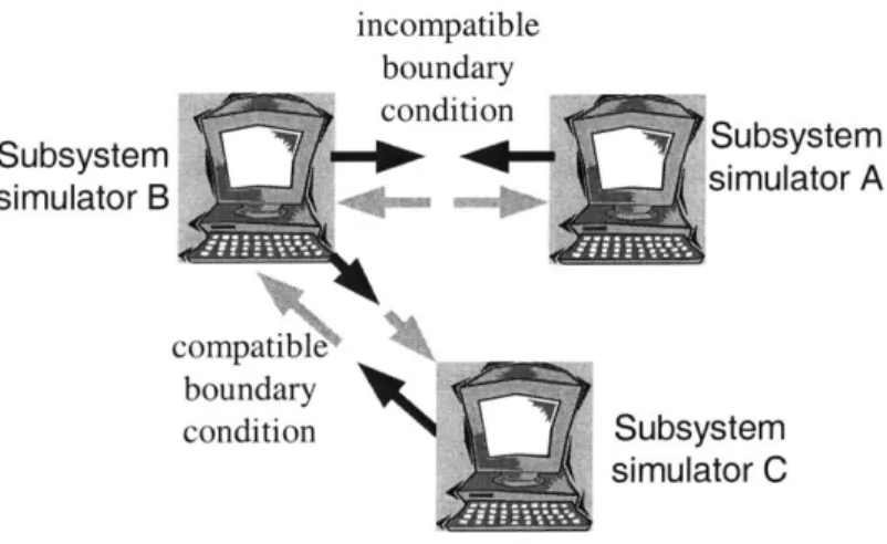
incompatible boundary dr e condition Subsystem -41 11 <Subsystem simulator B simulator A compatible boundary condition Subsystem simulator C

Figure 2.2.1 Co-Simulation of dynamic subsystems with different boundary conditions.

2.2

Algebraic Constraints

Power, the time rate of energy transfer, is the scalar product of the conjugate power variable-the flow variable

f

ein fin = eot foul. (2.2.1) We can also apply any one of the physical laws, such as Newton's third law, conservation of mass, conservation of momentum, conservation of electrical charge, etc., to the junction. Then boundary equation (2.2.1) can be written as

e(fin - fol) =0 (2.2.2)

or

(egn - eot,) f =0 . (2.2.3)

Suppose that we have two subsystems coupled in the common effort case of Eq. (2.2.2). If the boundary condition is compatible, i.e. u1, y1, U2, Y2 being e,

fou,

S= f(x, t), (2.2.4)

where x is the combination of x, and x2. The input is represented by the output of the other

system and is not explicitly shown in Eq. (2.2.4). This type of coupling is shown in Fig. 2.2.1 between subsystem B and C.

However, if the boundary condition is incompatible, i.e. uj, yl, U2, Y2 being e,

f,,

f

',

i =f(x, z,t) (2.2.5)

0= y1(x,u,t)-y 2(x,u,t)= g(x,z,t), (2.2.6) where z, called a constrained input, is the input u1 and u2 of the coupled subsystems. g is the

algebraic constraint that must be used to decide the constrained input z. This type of coupling is shown in Fig. 2.2.1 between subsystem the simulators A and B.

-~ - ~ -I - - -

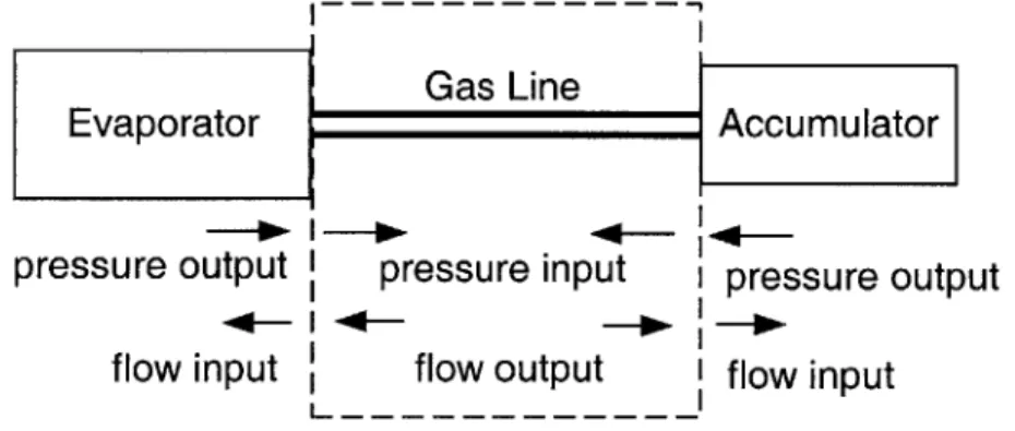
-Gas Line

Evaporator Accumulator

pressure output I pressure input I pressure output flow input flow output I flow input

Figure 2.2.2 Incompatible boundary condition caused by numerical difficulty.

In some cases, the original models are compatible at the interface, such as shown in Fig. 2.2.2. However, when the connecting pipe is short and wide or the mass flow rate is low, the static equation that calculates the flow based on pressure difference becomes nearly singular. The proximity to the singularity makes the pipe equation very sensitive to pressure difference and can therefore be quite error prone. In practice, the pressure drop between the heat exchanger and the condenser is ignored to preclude these potential errors. Without the pipe, though, the two thermal equipment models have to interact across an incompatible boundary condition.

Incompatible boundary conditions are the most significant source of algebraic constraints in the modeling of dynamic systems [Campbell, 1995]. Algebraic equations can also be the result of model reduction or constrained dynamics, etc. We focus on the algebraic constraints caused by the incompatible boundary condition in this research. The challenge is to develop a method that can numerically solve differential equations coupled with algebraic constraints without compromising the object-oriented properties of the subsystem simulators.

2.3

Differential Algebraic Equation and Index Reduction

A differential system constrained by an algebraic equation, such as

i = f(x, z,t) (2.2.5)

0 = g(x,z,t), (2.3.1)

is called a Differential Algebraic Equation (DAE). Assuming that the constraint equation (2.3.1) is sufficiently differentiable and that a well-defined solution for x and z exists with consistent initial conditions, i.e. initial condition satisfies the algebraic constraint equation, an important structural property of a DAE known as the index can be defined [Brenan et al, 1989]. The minimum number of times that all or part of the constraint equation (2.3.1) must be differentiated with respect to time in order to solve for as a continuous function of t, x, and z is the index of the DAE Eqs. (2.2.5) and (2.3.1).

Assuming that the DAE has an index r, by definition of the DAE index, the following set of algebraic equations must be satisfied by any exact solution of the DAE:

0 = g(x, z, t) (2.3.1) dg 0 = - (2.3.2) dt dr-i 0= ,r_ g. (2.3.3)

A new constraint equation can be defined as a weighted summation of Eq. (2.3.1) through (2.3.3). This new constraint equation requires only one differentiation to solve for . If we use this new constraint equation to replace the original constraint Eq. (2.3.1), the resulting DAE is index one

and it is thus easier to solve. We define the following equation as the previously mentioned weighted summation:

d ,r-1

s(x,t)= P -+1 g=0, (2.3.4)

dt

where p > 0. This is also known the Baugerte's stabilization [Baugarte, 1972]. This equation can be viewed as a sliding manifold as well. The sliding manifold definition places the poles of the constraint dynamics at -p-1 [Gordon and Liu, 1998]. Now the DAE system (2.2.5) and (2.3.4) is index 1 and is much easier to solve.

Equation (2.3.4) represents a critically damped dynamic system. There are (r-1)

decoupled linear modes in this dynamic system. The time constant of each mode is the same and is equal to u. If the sliding manifold equation is satisfied, all modes of the sliding manifold subspace decay to zero asymptotically with time constant U. The derivatives of the original algebraic constraint, and the weighted summation of the constraint and the derivatives will remain zero all the time if the original algebraic constraint Eq. (2.3.1) is satisfied at the beginning of the simulation. Thus the original high index algebraic constraint can be replaced by the reduced index algebraic constraint Eq. (2.3.4).

2.4

Resolving of Algebraic Constraints

In the past 30 years, many DAE solution algorithms and packages have been developed [Brenan et al, 1989; Mattsson and Soderlind, 1993; Petzold, 1983]. If we use the existing DAE solution packages, we have to collect all dynamic and algebraic equations from all of the subsystems and feed them into the DAE solution package. This approach can solve object-oriented modeled large systems, but it should not be used in the Co-Simulation environment since every subsystem simulator of the Co-Simulation is an object-oriented component. If we dismantle the subsystem simulators and extract models out, we destroy the basic building blocks of Co-Simulation and the object-oriented simulation paradigm is destroyed.

Another way of dealing with the DAE system is to convert the DAE system into an ODE system. This procedure, known as DAE realization in the control community, may increase or decrease the dimension of the system. Figure 2.4.1 shows one example of two subsystems coupled through incompatible boundary conditions. Because of the boundary conditions, the

overall system equations contain algebraic constraints. Subsystem A takes an effort input and produces a flow output. If we can change the causal assignment of the R element of subsystem A, subsystem A can take a flow input and produce an effort output. Therefore, by manipulating the subsystem model, the algebraic constraint can be eliminated as shown in Fig. 2.4.2.

S R: Rf R: RS

Ppf:Se-l[-Se TF Se Se I---C:CS

V 1/A coupling X

Subsystem B /A -x=O Subsystem A

Figure 2.4.1 Algebraic constraint.

If R: RjR : R -4

I:\ R:R1 R

Ppump:Se -- TF Se Sf--- 1-C: C,

Subsystem B Subsystem A

Figure 2.4.2 Algebraic constraint eliminated.

However, manipulating subsystem equations is against the functional requirements of the Co-Simulation since subsystems will be provided in the form of coded simulators. Also this method does not always work in practice. If R,-I is not given in a closed form expression, this method fails.

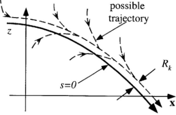
Figure 2.4.3 shows that two robots keep their endpoints in contact with each other. If we treat each robot as a subsystem simulator, we can simultaneously run two simulators of the robots to simulate the system. However, the boundary condition, which is the point of connection for the two endpoints, forms an algebraic constraint. We can add a fictitious spring and damper between the two endpoints empirically. This addition makes the original incompatible boundary condition compatible and thus removes the algebraic equation. Known as the stiff element method, this method does not change the subsystem simulators and the modularity is intact [Zeid and Overholt, 1995]. However, this approach requires an ad hoc procedure for tuning parameters. In practice, we can only adopt linear components for the fictitious spring and damper. The linear components substantially reduce the performance that the fictitious spring and damper may provide. Slightly damped linear stiff elements introduce

highly oscillatory modes while heavily damped linear elements converge to the algebraic constraint slowly.

Subsystem A Subsystem B

Figure 2.4.3. Fictitious spring and damper

A substantial improvement for the original ad hoc stiff element method is the Singularly Perturbed Sliding Manifold (SPSM) method [Gordon and Liu, 1998]. It is devised based on the nonlinear control theory. The algebraic constraint is treated as the desired trajectory and a model based feedback controller is designed to push the system onto the desired trajectory. Starting from the index-reduced DAE Eqs. (2.2.5) and (2.3.4), a boundary-layer-smoothed switching control law is used to enforce the sliding manifold Eq. (2.3.4)

s = -Ksat , (2.3.5)

where 1 >> e > 0 and K is a positive constant [Slotine and Li, 1991]. Since both s and i are known, we can solve for i using Eq. (2.3.5):

(asl

= (-K - I sat -- I -+--fi. (2.3.6)

az) (e) az at ax

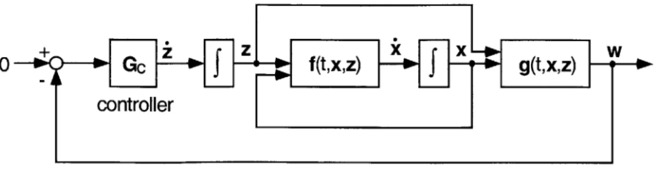
The ODEs in equations (2.2.5) and (2.3.6) are based on the realization of the DAE Eqs. (2.2.5) and (2.3.1). Figure 2.4.4 shows the block diagram of the SPSM realized DAE system [Gordon, B. W., 1999]. DAE realization using SPSM keeps the modularity of the subsystem simulators. The dynamic equation (2.3.6) can be viewed as the generalized fictitious spring and damper, which supplies the compatible boundary condition for the subsystem simulators.

00

0

GC

f(t,x,z)

g(tx~Z)--controller

Figure 2.4.4. Modeling the solution of DAE as a control system.

However, by replacing Eq. (2.2.5) with Eq. (2.3.6), we are using a stiff ODE system to approximate the original DAE system. The resulting stiff ODE system may be even harder to solve than the original DAE (2.2.5) and (2.3.1) [Brenan et al, 1989]. We not only have to stabilize the sliding mode by choosing appropriate parameters of e and K, but we must also guarantee the numerical stability of the resulting stiff ODE. The SPSM based control law is highly nonlinear and the subsystems are often nonlinear as well. Guaranteeing unconditional numerical stability for arbitrary nonlinear dynamic simulation is very difficult.

2.5

Pure Discrete-Time Boundary Condition Coordinator

The Singularly Perturbed Sliding Manifold method is a control-inspired realization method, which can provide the correct boundary condition stably. However, the SPSM method is a continuous-time approach. If we were to use the SPSM method in the Co-Simulation, we would have to check the numerical stability along with the stability conditions of the sliding mode since the Co-Simulation is a numerical simulation. Although subsystems of a coupled system are continuous systems, the subsystem simulators are all discrete-time systems. If the algebraic constraints are converted into stable discrete-time dynamic systems that provide the same boundary condition, we do not have to check the numerical stability.

Before we move on to the discussion of discrete-time systems, we first define a notation that will be required for our discrete-time analysis. All variables evaluated at time kAt are written with a subscript k. For example, the state variable x(kAt) is written as Xk and the

constrained input z(kAt + At) is written as Zk1. All functions evaluated at (Xk, tk, zk) are written

with subscript k. For example, the sliding mode S(Xk, tk, zk) is written simply as Sk. th

ii=f Xi, ui,t)

(2.5.1)

=i y(xi)

The simulator form of the dynamic subsystem is the discretized version of the above model

Xik+1 = Xi,k + At*i (2.5.2)

Yi,k+1 = Y(Xi,k+1)

where Xik _{is the effective derivative, which is different for different numerical integration}

methods. For the sake of simplicity, we use Euler's forward integration formula. The effective derivative in this case is simply

Xi,k i,k fi (Xi,k, zk, tk) (2.5.3)

Considering the case when two subsystems are in causal conflict configuration; the overall model of the coupled system is then

Xk+1 - Xk + At f(xk ,zk ,t ) (2.5.4)

0 = g(Xk+l) (2.5.5)

where z replaces u to emphasize the algebraic constraint. Using Eq. (2.3.4), we define a sliding manifold to replace the original algebraic constraint Eq. (2.5.5). So, the algebraically coupled dynamic system with the reduced index in the numerical simulation form is

Xk+1 -Xk +At-f(Xk,zktk) (2.5.4)

s(Xk+1,zk+1,tk+1)= 0. (2.5.6)

For this discrete-time system, the dynamic system is only meaningful at the sampling point tk and the constraint equation needs to be satisfied only at the sampling point as well.

We want to design a special discrete-time dynamic subsystem, which enforces the constraint equation (2.5.6) by providing the constrained input. This special subsystem simulator converts the incompatible boundary condition into a compatible boundary condition. Called a Boundary Condition Coordinator (BCC), the special subsystem simulator is a linear dynamic system

-1

Zk+1 - Zk + Vk, (2.5.7)

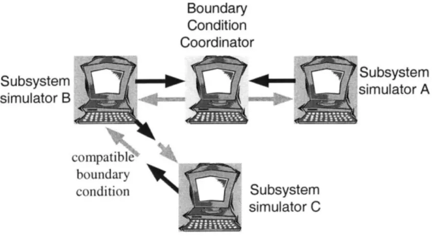
where Zk is the state variable of the BCC and vk is the control input, which we will design based upon the output variable Yk's from the two subsystem simulators that are connected through the algebraic constraint. Applying the BCC to the system with the incompatible boundary condition in Fig. 2.2.1, we have resolved the incompatible boundary condition as shown in Fig. 2.5.5.

Boundary Condition Coordinator Subsystem Subsystem simulator B simulator A compatible boundary condition Subsystem simulator C

Ill

Discrete-Time Sliding Mode

3.1

_{Introduction to Discrete-Time Sliding Mode Control}

An intuitive approach to Discrete-Time Sliding Mode (DTSM) control is to derive control laws in the continuous-time domain and implement them directly in the discrete-time domain. However, this straightforward method leads to discretization chatter as shown in

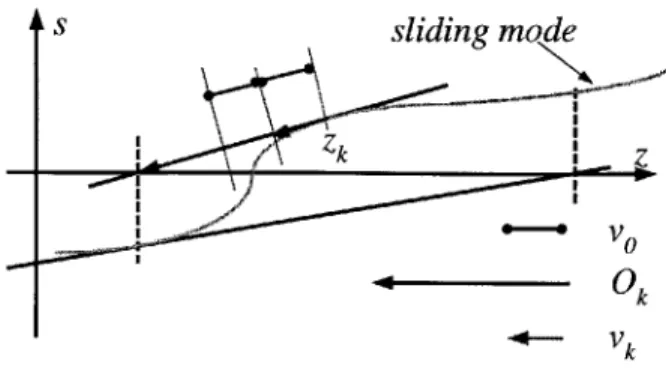
Fig. 3.1.1 [Yu, 1994]. The discretization, i.e. finite-frequency sampling, causes the discretization chatter. This type of chatter is not the result of the unmodeled dynamics. Figure 3.1.2 shows the sliding mode driven by an ideal infinite fast controller and shows no chattering problem. Because the straightforward approach to the discrete-time sliding manifold always causes the chattering phenomenon and the trajectory does not stay on the sliding manifold, this type of the discrete-time sliding mode is also called pseudo or quasi sliding mode [Delonga, 1989].

z A

pseudo sliding mj e

X

Figure 3.1.1 Pseudo sliding mode in the discrete-time domain.

For a continuous-time system, discontinuous control is required to make the dynamic system exhibit the sliding mode. However, discontinuous control is not required for a discrete-time dynamic system to exhibit the sliding mode motion [Drakunov and Utkin, 1992]. The definition of the discrete-time sliding mode is given by [Utkin et al, 1999]. In the discrete-time dynamic system,

where x E R", u e Rm, f: RnxRm -> _{R". The discrete sliding mode takes place on a subset I of} the manifold a= {x: s(x) = 01, s E Rm, if there exists an open neighborhood E of this subset such that for each x e E, it follows that s(xk+J) e 1.

sliding mode

x

Figure 3.1.2 Sliding mode in the continuous-time domain.

3.2

Single-Rate DTSM

3.2.1 Dynamics of the Sliding Function

The design of the Boundary Condition Coordinator is viewed as a control problem. The dynamic system in discrete-time is

Xk+1 X Xk + At f(xk, zk, tk) ₍(3.2.1)

(3.2-2) and the system trajectory should stay at, or close to, an equilibrium point:

S(Xk+1, Zk+1, tk+1) =0. (3.2.3)

The relative order of this stabilization problem is zero.

Assuming the continuous function s is sufficiently differentiable around the point s = 0, sk+I can be obtained as follows:

Zk+ =Zk +Vk ,

Sk+ = k +as _asx(Xk tk, Zk> (Xk+1 _{- Xk)+ as (Xi, tk, Zk ) -At}

at

as

az

where R is the second order remnant term. If we let w = [x , t, z]T, then Rk is as follows:

Sa (as T

Rk -Aw [ Awk, (3.2.5)

aw aw

-k +OAWk

where 0 0 ! 1, according to the Mean Value Theorem. Substituting in the dynamic equation (3.2.1) and (3.2.2), Equation (3.2.4) can be represented by using variables of step k, and we have

sk+1 sk + JXkAt-(xkZ,t)JtkAt+JZV+ R. (3.2.6) We define

as

_az

for the sake of notation clarity. The sliding function s at the step k+1 is

sk+1 = sk + ak + JZkVk + Rk. (3.2.9) By the definition of the DAE index, JZk is nonzero.

3.2.2 Continuous Control Input

From Eq. (3.2.9), we find that the discrete-time dynamic system s at the step k+1 is decided by four terms. Term Sk is the starting point for the next step. Terms ak and Rk are external influences applied to the dynamic system Eq. (3.2.9). Term JZkVk is where active control can be applied to influence Sk+.. In order to push Sk+J towards the equilibrium point, we have to ensure that the control influences the system more than other sources. Therefore, it intuitively requires a minimum magnitude for the control input such that the control input is always strong enough to compensate for the external influences and to push the system trajectory towards the right direction. _{vo is denoted as the magnitude of the minimum control input. A domain} DcQ={x,t,z~xe R",te R+,zE R} can be defined, and D is the vicinity of the sliding

manifold and the index is fixed. |JzL1,

Ia(At)|

vO > sup( Jz 1 _{) -sup(la(At)| + R(At,vo) + 6),}

D D

(3.2.10)

where the constant dis a small finite positive constant.

Since the term Rk cannot be exactly evaluated, we let the equivalent control Ok be our estimate of Vk that makes the next step of the sliding function, Sk+J, zero, giving

Ok =-J- (Sk +ak). (3.2.11)

We choose a control law

Vk = v₀ sat( .

VO (3.2.12)

The saturation function satO is used to limit the magnitude of the control input in order to guarantee the stability..

3.2.3 The Invariant Set around the Origin

We want to show that the closed-loop system with the control law of Eq. (3.2.12) possesses an invariant set

s supIR

D

(3.2.13)

around the origin s = _{0. When the system trajectory starts in the region that satisfies Eq. (3.2.13),}

we have

-Jzk '(sk + a < sup Jzi' -sup(RkI+ Iak1).

D D

The left hand side is actually the magnitude of the equivalent control Ok, so we have

Ok <maxJzk -max|RkI+-Iak1).

Adding one more term to right hand side and applying the inequality (3.2.10), we obtain

(3.2.14)

Ok< maxJz' -maxRkI + -akI +)< vo.

This shows that the control law becomes

Vk VO sat =O

(VO)

under the condition Eq. (3.2.13). Substituting the control input (3.2.17) into the discrete-time dynamic system (3.2.9), we have

Sk+1 - Sk +ak + JZk(- Jzk (Sk +ak))+ R =Rk. (2

This shows that Eq. (3.2.13) is an invariant set. attractive.

3.2.4 Proof of Convergence

Next we will show that the invariant set is

To prove that the invariant set around the origin is attractive, we choose a Lyapunov function candidate

V(tk,s )=V =|s| (3.2.19)

It is easy to find positive constants a and b > 0 such that

alsk| 1 Vk _{: bsk|.} (3.2.20)

This shows that the function V is positive define and decrescent. We define the forward difference function AV as follows:

AVk =Vk+1 -Vk =|sk+1|-ISk|. (3.2.21)

If the trajectory starts not far from the invariant set of Eq. (3.2.13)

sup Jz-- supRl) < ISk I< sup Jz-1 _{-sup(jRJ+ Ja),}

D D D D

(3.2.22)

it is easy to see that the sliding function s will reach the invariant set in one step of time. Now, let us start from

(3.2.16)

(3.2.17)

sliding mode

-4--z

I- -*

+- _Vk

Figure 3.2.1 Illustration of the equivalent control, minimum control magnitude and control input.

s > sup Jz- -sup(Rj + a),

D D

which is equivalent to

jOkj> V0.

Substituting Eq. (3.2.12) into Eq. (3.2.9) and applying Eq. (3.2.11), we have

sk+1 = sk +ak + JZkVO 1 + Rk

(3.2.25)

=Sk +ak + JZkVO -J (sk +ca ) +Rk

O1k

O

=(Sk+clk)l 1( - -I1-+Rk

We substitute Eq. (3.2.25) into the forward difference of the Lyapunov function candidate and we have

AVk =|sk+1|-sk|= (Sk + ak) r1 VO + Rk iskI -10k|I

(3.2.26)

Applying inequality (3.2.24), the forward difference function AVk can be written as:

(3.2.23)

(3.2.24)

s

S

AVk sk+a k|r1 Vo +|Rk|-|sk =jSk+ackI- k+|ak +R -|s Jzk' Sk + ak ) .+kR k(3.2.27) = sk +ak|- Vo +|JRk

|-|Jsk|

Combining Eq. (3.2.28) and Eq. (3.2.27), we finally arrive at:

AVk < -S <0. (3.2.29)

This result guarantees that the system trajectory moves towards the invariant set (3.2.13) at a finite rate and that the invariant set is asymptotically stable.

According to the theorem of the discrete-time sliding mode, the closed-loop system exhibits a discrete-time sliding mode after s reaches the invariant set of Eq. (3.2.13). Once the sliding mode is established, the system trajectory will stay within the invariant set forever. The invariant set is also called the boundary layer of the sliding manifold of Eq. (3.2.3). Figure 3.2.2 shows the motion of the discrete-time sliding mode.

The meaning of the bound equation (3.2.10) can be explained by Eq. (3.2.9). The magnitude of the control input vo must be large enough to compensate for ak and Rk to guarantee

Is+11

Xk, Zk, At, and vo. Although Rk is the second order small quantity with respect to At and vo, Rk can

still be large if s is highly nonlinear with respect to At or vo. When Rk is large, we need a large vo on the left hand side of Eq. (3.2.10) to compensate for the Rk effect. A large vo will in turn cause a larger Rk. This may make finding a vo satisfies Eq. (3.2.10) impossible.

However, we can always find a vo that satisfies the inequality (3.2.10) by reducing the step size At. When At is small, Eq. (3.2.10) can be written as follows:

vo > + , _(3.2.30)

where e and y are small positive numbers. This shows that we can always find vo that satisfies condition (3.2.10) and therefore the discrete-time sliding controller is able to stably enforce the algebraic constraint Eq. (3.2.3).

possible trajectory

x

Figure 2.2.2 Phase portrait of the discrete-time sliding mode motion.

3.3

The Multi-Rate DTSM

3.3.1 Two-Time Scale Problem

The cost of using a small At to satisfy the convergence condition in Eq. (3.2.10) is high, especially when the dimension of x is large. We have to decrease the step size for the entire coupled system just to guarantee the stability of the sliding controller designed for the incompatible boundary condition. Although, the smaller step size will make the accuracy of the entire system better, the extra accuracy gained in x by the smaller integration steps may not be necessary. Thus it is of great interest to decouple the overall step size of the Co-Simulation from the stability requirement of the sliding mode controller.

In physical system modeling, very fast dynamics are sometimes modeled as algebraic constraints since the time constants of the fast dynamics are much faster than the dynamics of the rest of the system. If we are not interested in the dynamic properties of the fast dynamics that settle in a very short period of time but rather in the slower dynamics, we can treat the fast dynamics as algebraic constraints [Kokotovic et al, 1986]. This is the basis of the singular

perturbation theory. For such cases, using the fast dynamics Eq. (3.2.2) to replace the algebraic constraint Eq. (3.2.3) makes physical sense. Some algebraic constraints are not the result of ignoring fast dynamics. They are the result of redundant state variables. Although replacing this type of algebraic constraint is not based on physical reasoning, the sliding control method that we have just shown shows that the error generated by the substitution can be controlled and small. In either case, the algebraic constraint can be viewed as a dynamic system that settles to a constant in a short time period, which is much smaller than the smallest time constant of the rest of the dynamic system. This suggests that we can simulate the algebraic-constraints-converted fast dynamics using a time step smaller than the integration step size of the subsystem simulators. This leads to multi-rate simulation.

3.3.2 Implementation of DTSM

To implement the multi-rate simulation, we divide one step of the subsystem simulators into n small steps. Now the integration of the subsystem simulators is in the time scale k, while the algebraic constraint is simulated in the time scale i which is n times faster than the time scale k. Any variable evaluated at At(k + i/n) instant is denoted using subscript k + i/n . When we calculate variables, such as s i and Jz i , the value of the state variable x i is required.

k+- k+-

k+-n n n

The true value of x _{cannot be obtained for every i from the subsystem simulators since the}

k+-n

state variables updates only at At -k instant. Instead, we use the values of Xk and Xk+1 to

interpolate the value of x i . In order to avoid clumsy notation, the variable name of x ; is

k+-

k+-n n

used for these interpolated values.

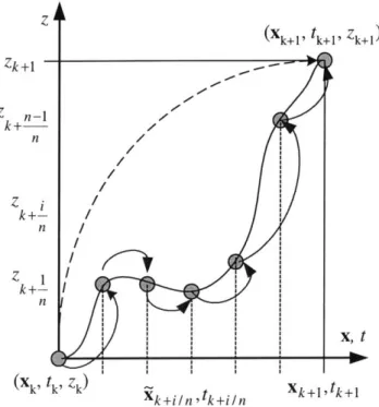
Figure 3.3.1 compares the new multi-rate method with the original single-rate method.

For Zk+J _{integration, we spend n small steps from Zk instead of just one step from Zk. By the}

configuration of this type of multi-rate scheme, we know that the sliding function s evaluated in the fast time scale can be used in the slow time scale. If we pick every s out of all s

k+-

k+-n n

when i is zero, we obtain the s series in the large time scale. This shows that if the sliding controller in the fast time scale is stable, then the sliding controller in the slow time scale is also stable.

(xk+1' tk+1' Zk+1 Zk+1 - -n k / n/ Z I n X, t Xk' Ak' Zk _Xk+1'tk+1 Xk+i/n,tk+i/n

Figure 3.3.1 Possible implementations of the multi-rate algorithm. Similar to the previous proof, we can define a Lyapunov function candidate

V i = s i , (3.3.1)

k+-

k+-n n

and this function also has the property of Eq. (3.2.5). The forward difference of the Lyapunov function candidate is

AV i = s i+₁ - s . (3.3.2)

k+- k+--

k+-n n n

s i+1 is obtained by the local linearization and the interpolation of x, as follows k +-n as Axk as At as s i+1=s i+ +-- .- +-- Azi k+- k+- X k+1 at k+ aZk+- k+-n n n n n n n n n(3.3.3) +R i tk+-At,xk+---Ax,z i,---, Az i k+ n n k+- n k+-n yn n

Similar to Eq. (3.2.9), the sliding mode at k + i+! step is

n

s i+1 =s ; +a i+Jz ; -v +R . (3.3.4)

k+ k+ k+- k+- k+-

k+-n n n n n n

The equivalent control is

0 =-JzI S +a (3.3.5)

k+ k+- k+-

k+-n n n ny

and the control law is

k+-v k+ = vo sat "O . (3.3.6)

n

We can also show that

s| sup(R|). (3.3.7)

D

is an invariant set if the system is under feedback control law (3.3.6). We need to find what condition vo has to satisfy in this multi-rate scheme. Starting from the initial condition

0 i > vO, (3.3.8)

k+-n

and using the procedure similar to Eqs. (3.2.25) to (3.2.27), it requires that

a _k+- +R _{k +-_} vo 0 < (3.3.9)

n n Jzi

k

+-n