HAL Id: hal-01081031
https://hal.inria.fr/hal-01081031
Submitted on 30 May 2017
HAL is a multi-disciplinary open access
archive for the deposit and dissemination of
sci-entific research documents, whether they are
pub-lished or not. The documents may come from
teaching and research institutions in France or
L’archive ouverte pluridisciplinaire HAL, est
destinée au dépôt et à la diffusion de documents
scientifiques de niveau recherche, publiés ou non,
émanant des établissements d’enseignement et de
recherche français ou étrangers, des laboratoires
Amortized Õ(|V|) -Delay Algorithm for Listing
Chordless Cycles in Undirected Graphs
Rui Ferreira, Roberto Grossi, Romeo Rizzi, Gustavo Sacomoto, Marie-France
Sagot
To cite this version:
Rui Ferreira, Roberto Grossi, Romeo Rizzi, Gustavo Sacomoto, Marie-France Sagot. Amortized Õ(|V|)
-Delay Algorithm for Listing Chordless Cycles in Undirected Graphs. 22th Annual European
Sym-posium on Algorithms, Sep 2014, Wroclaw, Poland. pp.418-429, �10.1007/978-3-662-44777-2_35�.
�hal-01081031�
Amortized ˜
O(|V |)-Delay Algorithm for Listing
Chordless Cycles in Undirected Graphs
Rui Ferreira1, Roberto Grossi2, Romeo Rizzi3, Gustavo Sacomoto4, and
Marie-France Sagot4
1
Microsoft Bing, UK
2 Universit`a di Pisa, Italy 3
Universit`a di Verona, Italy
4
INRIA Grenoble Rhˆone-Alpes, France & Universit´e Lyon 1, France
Abstract. Chordless cycles are very natural structures in undirected graphs, with an important history and distinguished role in graph theory. Motivated also by previous work on the classical problem of listing cycles, we study how to list chordless cycles. The best known solution to list all the C chordless cycles contained in an undirected graph G = (V, E) takes O(|E|2+|E|·C) time. In this paper we provide an algorithm taking
˜
O(|E| + |V | · C) time. We also show how to obtain the same complexity for listing all the P chordless st-paths in G (where C is replaced by P ).
1
Introduction
A chordless (induced) cycle c in an undirected graph G is a cycle such that the subgraph induced by its vertices contains exactly the edges of c. A chordless cycle is called a hole when its length is at least 4. Similarly, a chordless (induced) path π in G is such that the subgraph of G induced by π contains exactly the edges of π. Both chordless cycles and paths are very natural structures in undirected graphs with an important history, appearing in many papers in graph theory related to chordal graphs, perfect graphs and co-graphs (e.g. [11, 6, 3]), as well as many NP-complete problems involving them (e.g. [2, 7, 9]).
In this paper we consider algorithms for listing chordless cycles and st-paths in a undirected graph G = (V, E), with n = |V | vertices and m = |E| edges, motivated by the algorithms for listing cycles and st-paths that have been pro-duced by an active area of research since the early 70s [10, 13, 1]. In this paper we present an algorithm for listing all the C chordless cycles in an undirected graph G = (V, E) in ˜O(m + n · C) time, hence with an amortized ˜O(n) time de-lay, where ˜O(f (n, m)) is used as a shorthand for O(f (n, m) polylog n). We also show that the same algorithm may be used to list all the P chordless st-paths
˜
O(m + n · P ) time, hence amortized ˜O(n) time delay.
There are very few algorithms in the literature for listing chordless cycles and/or paths, where some of them have no guaranteed performance [12, 16]. The most notable and elegant listing algorithm is by Uno [15], with a cost of O(m2+ m · C) time for chordless cycles and O(m2+ m · P ) time for chordless
2
Preliminaries
Our graphs are finite, undirected, and simple, i.e. without self-loops or parallel edges. Given a graph G = (V, E) with n = |V | vertices and m = |E| edges, our task is to list out fast all its chordless cycles. We hence assume that G is connected. Where V0 ⊆ V , we denote by EhV0i := {uv ∈ E | u, v ∈ V0} the
set of those edges which are contained in V0. A graph G0 = (V0, E0) is called a subgraph of G if V0 ⊆ V and E0 ⊆ E. The subgraph G0 is called induced (or
chordless) if E0 = EhV0i. For any V0 ⊆ V , we denote by G[V0] := (V0, EhV0i)
the subgraph of G induced by V0. Where e ∈ E, we denote by G \ e := (V, E \ {e})
the subgraph obtained from G by deleting the edge e. Where v ∈ V , we denote by G \ v := G[V \ {v}] the subgraph obtained from G by first deleting all the edges incident to v, and then removing the isolated vertex v. Given a vertex u ∈ V , we denote by NG(u) := {v ∈ V | uv ∈ E} the neighbourhood of u, the
subscript is omitted whenever the graph is clear from the context.
A cycle is a connected graph in which every vertex has degree 2. A path is a connected graph in which every vertex has degree 2 except for two degree 1 vertices, s and t, called the endvertices of the path. This is also called an st-path and denoted by π = s t. Indeed, when buiding a path from s to t edge after edge, it will be most natural, and more precise, to think like we are orienting the traversed edges. For this reason, we will also write (u, v) for an edge that, when buiding a path, has been traversed from u to v.
A (chordless) path (or cycle) of G is a (chordless) subgraph of G which is a path (or cycle). We denote by C(G) the set of all chordless cycles in G. We denote by P(G) (by Pst(G)) the set of all chordless paths (st-paths) in G. When
s = t, we get those cycles visiting s. We refer to a path π ∈ P(G) by its natural sequence of vertices or edges. An hole is a chordless cycle of size at least 4. Thus C(G) comprises holes and triangles. Since the triangles are at most mn, our algorithm can be used to list the holes of G in ˜O(n) time each, with an overall
˜
O(mn2) additive time cost.
Uno [15] proposed an algorithm that lists each chordless cycle in an undi-rected graph G = (V, E) in O(m) time while using O(m) space. The first step is the following reduction to the enumeration of chordless st-path in G. Based on the fact that for any vertex s ∈ V the chordless cycles in G \ s are also chordless cycles in G, the algorithm proceeds by listing all chordless cycles passing through s; and repeating the process in G \ s, until the graph is empty. Then, to list all chordless cycles passing through s in G0= G, the algorithm follows the approach of listing the chordless paths s t in G0\ (s, t), for each t ∈ NG0(s); and to
avoid duplications, at the end of iteration the graph is updated G0= G0\ t.
Given a previously computed chordless st-path π = v0v1. . . vk, Uno’s
algo-rithm identifies the set of vertices U ⊆ V such that each u ∈ U is adjacent to some vi ∈ π, and the edge (vj, u) is contained in a chordless st-path extending
the prefix πj = v0v1. . . vj different from π. The algorithm is kick-started by
taking the shortest st-path (as the shortest path has the property of also being a chordless path) and employs a recursive strategy of vertex removal to avoid listing the same chordless path multiple times. This ensures that each chordless
path is listed once. Uno’s algorithm takes O(m) time to compute U and prepare the recursive calls before it either outputs a new path or stops. The total time is therefore O(m2+ m · |C(G)|).
3
Our Approach and Key Ideas
We outline the main ideas which allow us to reduce the amortized cost for a chordless path from O(m) to ˜O(n), giving a total ˜O(m + n · |C(G)|) time to list all the chordless cycles. Our approach relies on a variant of the cleaning operation introduced in [6] to recognize linear balanced matrices and even holes in graphs [4, 5].
3.1 Certificates for chordless st-path
A listing algorithm usually takes the form of a recursive procedure exploring the space of all solutions. A key idea employed since the first listing papers [10] is to check for the existence of at least one solution before branching, i.e. before partitioning the solution space in subspaces to be assigned to the children. This avoids unproductive recursive calls as they do not list any solutions but their overhead cost can completely dominate the cost of reporting the solutions (e.g. see [14]). In a previous work [1], we stressed the notion of certificate since, in a more refined recursive scheme, passing a certificate of existence as an extra parameter may facilitate the work of the children which may avoid running the existence check: if they have a single child, they could be done by just passing the certificate received in input or a small adaptation of it. We also saw that more structural facts around the certificate could be useful. For the case of st-paths [1], the certificate is a DFS tree rooted in s and reaching t, which contained an st-path and also helped in other ways. Until now, the certificate was also a solution itself or contained one.
Here we try out something new: what if our certificate guarantees the exis-tence of a solution but is not itself a solution? The following fact suggests that the certificate for the existence of a chordless st-path might be just any st-path. Fact 1 Given two vertices s, t in G, there is a chordless st-path in G iff there is an st-path in G.
Thus we allow for certificates which are somewhat less refined than actual so-lutions, in the same spirit that a binary heap demands a less strict and lazy notion of order. This is a new asset of the notion of certificate and opens up new possibilities.
3.2 From chordless cycles to chordless st-paths
Uno [15] shows how to reduce listing chordless cycles in a graph to listing chord-less st-paths for all edges (s, t) chosen in a specific order (see Section 2), which
is necessary to avoid duplications in the output. The initialization step for each edge (s, t) takes O(m) time as it requires to find one chordless st-path. This gives the m2term in the total cost of O(m2+ m · |C(G)|) for chordless cycles.
We observed in Section 3.1 that any st-path will suffice as a starter, as they are our certificates of choice. This makes a difference for the above reduction since using dynamic graph connectivity algorithms [8], it is possible to maintain a spanning tree in O(polylog n) time per edge deletion, perform connectivity queries in O(polylog n), and more importantly obtain an st-path in ˜O(n). It is worth noting that it is not known how to obtain a chordless st-path faster than O(m). Hence, we first build the dynamic connectivity structure as preprocessing step. Then, for each edge (s, t), in the same order as Uno’s reduction, we list the chordless st-paths. Before calling our path listing algorithm for edge (s, t), we test if s and t are connected (Fact 1): if so, we call our path listing algorithm, paying ˜O(n) to find one initial st-path; otherwise, we skip the edge (s, t) and take the next in order. As a result, the total initialization cost is ˜O(m + kn) for all edges instead of O(m2), where k is the number of edges for which we find
one initial st-path. Note that k ≤ |C(G)| as each of them surely gives rise to a chordless st-path and, so a distinct chordless cycle. We obtain in this way an
˜
O(m + n · |C(G)|) time algorithm to list chordless cycles, if we can list st-paths in amortized ˜O(n) time each.
3.3 Difficulty of cleaning st-paths
Given any path, we can clean it as stated in Fact 1 to obtain a chordless st-path in a greedy fashion: start from u = s and iteratively take a neighbour of u that is closer to t along the path. The process stops when u = t. The vertices taken in this way form a chordless path. The problem is that the cost of such a greedy traversal of the path is upper bounded by the sum of the degrees of the vertices along it. Unfortunately, this sum could be Θ(m) in the worst case.
x1 p1 x2 p2 x3 p3 x4
Fig. 1. Sum of degrees on chordless path x1, p1, x2, p2, . . . , xr−1, pr−1, xr is Θ(m).
Even worse, this is still true when the initial path is already chordless, as shown in Fig. 1. Consider the complete bipartite clique Kr,r = (V1∪ V2, E12),
where V1= {x1, x2, . . . , xr}. Build a new graph G = (V, E) where the vertex set
is V = V1∪ V2∪ {p1, . . . , pr−1} for some new vertices p1, . . . , pr−1, and the edge
the path x1, p1, x2, p2, . . . , xr−1, pr−1, xris chordless but each edge is incident to
at least one vertex in that path, so the sum of the degrees is m = |E| = Θ(r2) =
Θ(|V |2) = Θ(n2).
What we would like to do: recursively extend a given chordless path πsuinto
a chordless st-path, while maintaining as a certificate an st-path. The recursive extension can be seen as an implicit cleaning of our st-path certificate. Consider a vertex u along a given st-path (our certificate), where initially u = s. Our certificate guarantees that there is at least one chordless st-path going through a neighbour of u, say a. However, we cannot explore all of u’s neighbours, so consider any neighbour b 6= a, the following two situations may occur. (1) a and b are both good, meaning that (u, a) and (u, b) are on two distinct chordless st-paths. In this case, the chordless st-paths traversing (u, a) cannot go through b too, as otherwise it would not be chordless (see Remark 1 below), so b should be removed. (2) b is not on any chordless st-path, so it is either disconnected from t or every st-path going through b passes through a. In this case, as it will be clear later, we need neither to explore nor to remove b.
In other words, we can treat the neighbours of u as described above, and they will not interfere when cleaning the st-path in the next recursive calls. We make this statement more precise below.
3.4 Reduced degree property
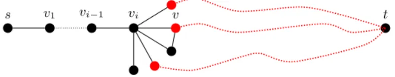
We introduce a notion of reduced degree with a stronger property in mind. Consider a chordless st-path πst = v0v1. . . v` in the graph G, for some integer
` > 1, where v0 = s and v`= t. For a vertex vi, a neighbour v ∈ N (vi) is good
if there exists a chordless st-path in G with prefix v0v1. . . viv (i.e. it extends
v0v1. . . vi by adding the edge (vi, v) as illustrated in Fig. 2). We denote by
Ngood(v
i) ⊆ N (vi) the set of good neighbours of vi, noting that vi+1∈ Ngood(vi).
For each vi, its reduce degree di is given by the number of non-good neighbours,
namely, di= |N (vi) \ (Ngood(vi) \ {vi+1})|.
s v1 vi−1 vi v t
Fig. 2. Good neighbours (in red) of vertex viin Gi.
The rationale is that exploring the good neighbours of vi will list further
chordless paths while examining its neighbours that are not good is a waste of computation. The reduced degree of viis actually an upper bound on the number
of not-good vertices examined when exploring vito produce the chordless st-path
πst and gives an upper bound on the waste. We now prove Lemma 1 below, as
path still takes O(m) time, only O(n) neighbours are a waste while the remaining ones lead to further chordless paths (which is a good argument for amortization). Lemma 1. For a chordless path πst, we havePvi∈πstdi≤ 2n, where di is the
reduced degree of vi∈ πst.
Proof. Consider a vertex x ∈ G that is a non-good neighbour of both vi and vj
for i 6= j. We can assume wlog that i < j. Moreover, we choose the vertices vi, vj
and x such that the difference j − i is the largest. Let us assume by contradiction that vi and vj are not adjacent in πst. We have that (vi, vj) is not an edge of G,
and x /∈ πst, since πstis chordless. We claim that the path π∗= v0. . . vixvj. . . vl
is a chordless st-path, contradicting the fact that x is not a good neighbour of vi. Clearly, π∗contains no repeated vertices, it is indeed an st-path. Let us prove
that it is also chordless. This follows from the fact that there is no vk∈ π∗, k 6= i
and k 6= j, such that (vk, x) is an edge of G, otherwise j − k or k − i would be
strictly larger than j − i, contradicting our choice of vi, vj and x. Hence, vi and
vj are adjacent in πst. Each vertex of G is therefore a non-good neighbour of at
most two vertices in πst. ut
3.5 Cleanup of current vertex
Suppose that we are exploring vertex u and we want to clean it as described in the previous sections. We identify a good vertex v, which closer to t along the st-path than the other neighbours. Ideally, we would like to throw away all the other neighbours of u but this cost gives O(m) per chordless path as illustrated in Fig. 1 and discussed in Section 3.3. We perform a partial cleaning, called cleanup, which consists in identifying, among all neighbours of u (i.e. |N (u)| elements) only its set Ngood(u) of good ones.
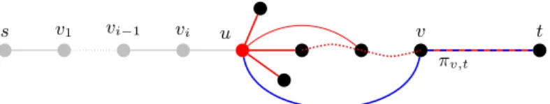
For a given u in a chordless st-path πst = v0. . . viu . . . vl, we let emerge
the good neighbours in Ngood(u) one by one as follows. Consider the graph G0
where the vertices v0. . . vi and its good neighbours were removed. If u and t
are not connected, then there cannot be further chordless paths from u and so there cannot be further good neighbours. Otherwise, if u and t are connected, we take any path from u to t, and select its neighbour v that appears along the path and is closer to t, as illustrated in Fig. 3. After that, we remove v and its incident edges, and iterate what described above until u is disconnected from t. The vertices v thus selected form the set Ngood(u) of good neighbours.
s v1 vi−1 vi u v t
πv,t
Lemma 2. For a chordless path πst, the cleanup of vertex u ∈ πst correctly
produces the set Ngood(u) of its good neighbours.
4
Listing Algorithm
We blend the key ideas discussed in Section 3 to get Algorithm 1, which has four parameters as input and lists all the chordless st-paths: the first parameter is the chordless path πsupartially built from s to the current vertex u (initially,
u = s), which is the second parameter; the third parameter is a ut-path πut
that is introduced following Fact 1; the fourth parameter is the reduced graph G, which changes with the recursive calls.
Algorithm 1: list induced pathss,t(πsu, u, πut, G) 1 if u = t then
2 output(πsu)
3 else
4 S := ∅
5 while true do
6 v := the vertex in πut∩ N (u) that is closer to t
7 πvt:= the subpath of πutfrom v to t
8 S := S ∪ {(v, πvt)}
9 remove v and its incident edges from G
10 if u and t are not connected then break
11 πut:= any path from u to t
12 end
13 foreach (v, πvt) ∈ S do
14 adds back v and its incident edges to G
15 list induced pathss,t(πsu· (u, v), v, πvt, G)
16 remove v and its incident edges from G
17 end 18 end
The algorithm outputs a chordless st-path if u = t (line 2). Otherwise, it performs a cleanup of u (the loop at lines 5–12). After that, it explores only the good neighbours recursively as they will surely lead to further chordless paths (the other loop at lines 13–17). Observe that S stores the good neighbours v of u and a vt-path for each of them: when performing the recursive call at line 15, only one of the vertices in S appears in the reduced graph G passed as a parameter to the recursive call (see lines 14 and 16 that guarantee this, and Remark 1 below). Hence, the recursive call now has as parameters the chordless sv-path πsu· (u, v)
ending in v, and a vt-path that guarantees that a chordless st-path exists and has πsu· (u, v) as a prefix: all the chordless st-paths in the reduced graph share
v0 v1 v2 v3 v4 v5 v6 v0 v2 v4 v1 v3 v5
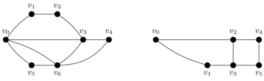
Fig. 4. Two example graphs where s = v0and t = v4.
For example, let us run Algorithm 1 on the input graph shown on the left of Fig. 4, with u = s = v0 and the initial path πut = v0v1v2v3v4. It computes
the pairs (v, πvt) in S as follows. First, (v3, v3v4) is added to S as v3 is a good
neighbour for v0 (the neighbour closer to t in the path), and the edges incident
to v3are removed. After this removal, s = v0is still connected to t = v4through
the path v0v5v6v4, which becomes the input for the next iteration of the while
loop. Next, (v6, v6v4) is added to S as v6 is another good neighbour, and the
edges incident to v6are removed and disconnect s from t, so the while loop ends.
The recursive calls in the foreach loop give the two chordless paths v0v3v4 and
v0v6v4 contained in the graph.
Remark 1. It is important to run the recursive calls with all good neighbours in S removed except one. If we left two or more good neighbours in the recursive call of line 15, they could interfere with each other and we might not obtain the chordless paths correctly. A very simple example is given in the graph shown on the right of Fig. 4. Consider for instance the case where Algorithm 1 would be given as input the path v0v1v3v2v4. The pair (v2, v2v4) is added to S and v2
removed. After that, the path v0v1v3v5v4 is found and the pair (v1, v1v3v5v4) is
added to S and v1 removed. Since v0 and v4 become disconnected, S contains
all the good neighbours of v0. Algorithm 1 executes the recursive calls with S.
Suppose that we keep both good neighbours v1and v2in G during these calls, in
particular for the call with the pair (v1, v1v3v5v4) from S. This call will extend
in a nested call the chordless path to πsu = v0v1v3 for u = v3, and will claim
that the good neighbours of v3 are v2 and v5, which is incorrect since v0v1v3v2
is not chordless. This situation does not arise if v2 is kept deleted in G when the
recursive call on v1 is performed as done in Algorithm 1.
The correctness of Algorithm 1 follows mostly from Lemma 2. Recall that, it guarantees that for a given path prefix πsuthe set S contains the good
neigh-bours of u, i.e. the neighneigh-bours of u that belong to at least one chordless st-path extending πsu. Clearly, we only have to recursively call the algorithm for these
neighbours, the others certainly lead to no solution. This implies that Algo-rithm 1 tries all the possibilities to extend πsu, so all chordless st-paths are
output. Moreover, since each good neighbours of u lead to a different extension, we have that no st-path is output more than once.
Certainly only st-path are output by Algorithm 1, but at this point we have no guarantees that the paths are indeed chordless. In fact, after building S, the algorithm proceeds to recursively extend the prefix πsu(u, v) for each v ∈ S in
the graph G0 = G \ (S \ {v}). However, since u was included in current path none of its neighbours can be used later in the recursion. The algorithm removes the good neighbours of u from G, but the other neighbours, NG(u) \ S, are still
present in G0. They could thus be used to extend the path later in the recursion, resulting in a non-chordless st-path. Lemma 3 shows that this cannot happen. Lemma 3. The st-paths output by Algorithm 1 are chordless.
The previous lemma leads to the following theorem.
Theorem 1. The algorithm correctly outputs all chordless st-paths of G. Theorem 2. The algorithm takes O(m + |Pst(G)|(tp+ ntq+ ntu)) time, where
tp is the cost of choosing any path from any two given vertices, tq is the cost
of checking if any given two vertices are connected or not, and tu is the cost of
removing/adding back any given edge. Proof. See Section 5.
There are several dynamic data structures in the literature [8] that main-tain a spanning forest for a dynamic graph, supporting insertions and dele-tions of edges in polylogarithmic time. Consequently, tp = O(n polylog (n)),
tq= O(polylog (n)), and tu= O(polylog (n)), thus giving the following bound.
Corollary 1. The algorithm takes ˜O(m + |Pst(G)| · n) time to report all the
chordless st-paths.
5
Amortized Analysis
Before starting our analysis, we observe some simple properties of the recursion tree generated by Algorithm 1.
Fact 2 The recursion tree R of Algorithm 1 has the following properties: 1. There is a one-to-one correspondence between paths in Pst(G) and leaves in
the recursion tree.
2. There is a one-to-one correspondence between proper prefixes of paths in Pst(G) and internal nodes in the recursion tree.
3. The number of branching nodes is |Pst(G)| − 1.
4. The length of a root-to-leaf path is equal to the length of the chordless st-path corresponding to the leaf. In particular, the height of the tree is ≤ n. Fact 2 suggests us to follow the following overall strategy.
1. We analyze the cost of each type (leaf, unary and branching) of node sepa-rately.
2. We consider all branching nodes together, and show that their amortized cost is O(tp+ tq+ ntu+ n) = ˜O(n) per solution.
3. We consider all unary nodes together, and show that their amortized cost is O(|πst|tq+ ntu) = ˜O(n) per solution.
4. We deduce that the cost of each solution is O(tp+ ntq+ ntu) = ˜O(n).
Lemma 4. The cost of a leaf is O(|πst|).
Let us now analyze the cost of the unary nodes. Let r = hπsu, u, πut, Gi be
a unary node. The vertex v ∈ N (u) is the only neighbour of u that can extend the prefix πsuinto a chordless st-path. Thus, removing v from G disconnects u
from t, and the algorithm performs a single iteration of the loop in line 5, not executing line 11. In this case, the algorithm performs the following operations: (i) one connectivity query (line 10), (ii) |N (v)| edge update operations on G (lines 9, 14 and 16), and (iii) a scan in the intersection of N (u) and πut to find
v (line 6). The cost of (i) and (ii) is O(tq+ |N (v)|tu).
A naive implementation of (iii) takes O(|N (u)|+|πut|) time, which is too large
to fit in our amortization strategy. In order to reduce this cost to O(|N (u)|) we therefore maintain, as an extra invariant, for each vertex in the current graph its the distance to t in the path πut. In this way, we can find v simply scanning N (u).
Thus, assuming the distance information is correctly maintained, we complete the proof of Lemma 5.
Lemma 5. The cost of a unary node is O(tq+ |N (v)|tu+ |N (u)|), where (u, v)
is the edge added to the chordless path.
It is not hard to maintain the distance information for hπsu(u, v), v, πvt, G0i,
the only child of the unary node hπsu, u, πut, Gi. As the path πvt is a suffix
of πut, the distance of the vertices in πut do not change. On the other hand,
the only vertices that the distances can change are the ones in πvt but not
in πut. These vertices can be identified when scanning N (v) in the child node
hπsu(u, v), v, πvt, G0i, since their distance is strictly larger than |πvt|. It remains
to show that the distance information can be maintained in the branching nodes. Lemma 6 shows that this is indeed the case, and gives an upper bound on the cost of the branching nodes.
Lemma 6. The cost of a branching node r ∈ R is O(β(r)(tp+ tq+ ntu)), where
β(r) is the number of children of r.
It remains to prove that we can maintain the distance information in branch-ing nodes in the same time bound of Lemma 6. This follows from the fact that in each iteration of the loop (line 5) we already paying O(|πut|), i.e. a full traversal
of the path πut. Before each recursive call in line 15 we can traverse the path πut
adding for each vertex the distance information, i.e. their position in the path. At this point we have bounds for the cost of each node in the recursion tree. However, by directly applying them we cannot achieve our goal of ˜O(n) time per solution. For instance, consider the particular case where all internal
nodes of the recursion tree are branching. The cost of each internal node is O(β(r)(tp+ tq+ ntu)) = ˜O(n2), since β(r) = O(n) in the worst case. Then, from
item 3 of Fact 2, the number of branching nodes is |Pst(G)| − 1. The total cost
for the tree is thus ˜O(|Pst(G)|n2) or ˜O(n2) per solution.
In order to get a tighter bound for the total cost of the branching nodes, we use the following amortization strategy. Let r ∈ R be a branching node. We divide the cost O(β(r)(tp+ tq + ntu)) among the closer descendents that are
branching nodes or leaves (no unary nodes), each being charged O(tp+ tq+ ntu).
This can always be done since r has β(r) children and the subtree of each child contains at least one leaf, i.e. the node r has at least β(r) non-unary descendants. In this way, the original cost of node r is completely charged to its non-unary descendants, and the only cost that remains associated to r is the one received from its ancestors. Finally, each branching node can only be charged once, by its lowest non-unary ancestor. Each branching node and each leaf is therefore charged with O(tp+ tq+ ntu). Thus, the total cost of the branching nodes is
O(|Pst(G)|(tp+ tq+ ntu)), completing the proof of Lemma 7.
Lemma 7. P
r:branchingT (r) = O(|Pst(G)|(tp+ tq+ ntu)).
Let us now bound the total cost of the unary nodes. Similarly to the branching nodes case, a straightforward use of the bound given by Lemma 5 leads to an
˜
O(n2) cost per solution, since in the worst case the recursion tree can have O(n)
unary nodes for each leaf. The key idea to obtain a better amortized cost is to consider the bound on the reduced degrees given by Lemma 1.
We first observe that each unary node is contained in some root-to-leaf path in the recursion tree. Thus,
X r:unary T (r) ≤ X l:leaf X r∈root l T (r). (1)
Fact 2 implies that there is a one-to-one correspondence between the pre-fixes of paths in Pst(G) and nodes in the recursion tree. That is, the each leaf
corresponds to a solution, and the root-to-leaf path root l corresponds to the chordless st-path associated to the leaf l. We can thus rewrite the double sum as X l:leaf X r∈root l T (r) = X π∈Pst(G) X vi∈π (tq+ |N (vi)|tu+ |N (vi+1)|). (2)
For each chordless st-path πst = v0. . . vivi+1. . . vk in the internal sum of
Eq. 2, we have that the degrees are actually the reduced degrees of Section 3.4, since the good neighbours (i.e. the set S in Algorithm 1) are always removed. Using Lemma 1 we can thus bound the sum of the degrees by 2n. Therefore,
X
r:unary
T (r) ≤ X
π∈Pst(G)
(|π|tq+ 2ntu+ 2n), (3)
completing the proof of Lemma 8. Lemma 8. P
r:unaryT (r) = O(
P
π∈Pst(G)|π|tq+ ntu).
References
1. Etienne Birmel´e, Rui A. Ferreira, Roberto Grossi, Andrea Marino, Nadia Pisanti, Romeo Rizzi, and Gustavo Sacomoto. Optimal listing of cycles and st-paths in undirected graphs. In SODA 2013, 1884–1896. ACM/SIAM, 2013.
2. Yijia Chen and J¨org Flum. On parameterized path and chordless path problems. In IEEE Conference on Computational Complexity, pages 250–263, 2007.
3. Maria Chudnovsky, Neil Robertson, Paul Seymour, and Robin Thomas. The strong perfect graph theorem. Annals of Mathematics, 164:51–229, 2006.
4. Michele Conforti, G´erard Cornu´ejols, Ajai Kapoor, and Kristina Vuskovic. Recog-nizing balanced 0, +/- matrices. In SODA 1994, 103–111. ACM/SIAM, 1994. 5. Michele Conforti, G´erard Cornu´ejols, Ajai Kapoor, and Kristina Vuskovic. Finding
an even hole in a graph. In FOCS 1997, 480–485. IEEE Computer Society, 1997. 6. Michele Conforti and M. R. Rao. Structural properties and decomposition of linear
balanced matrices. Math. Program., 55:129–168, 1992.
7. Robert Haas and Michael Hoffmann. Chordless paths through three vertices. The-oretical Computer Science, 351(3):360 – 371, 2006.
8. Bruce M. Kapron, Valerie King, and Ben Mountjoy. Dynamic graph connectivity in polylogarithmic worst case time. In SODA, pages 1131–1142, 2013.
9. Ken-ichi Kawarabayashi and Yusuke Kobayashi. The induced disjoint paths prob-lem. In Andrea Lodi, Alessandro Panconesi, and Giovanni Rinaldi, editors, IPCO, volume 5035 of Lecture Notes in Computer Science, pages 47–61. Springer, 2008. 10. R C Read and Robert E Tarjan. Bounds on backtrack algorithms for listing cycles,
paths, and spanning trees. Networks, 5(3):237252, 1975.
11. D. Seinsche. On a property of the class of n-colorable graphs. Journal of Combi-natorial Theory, Series B, 16(2):191 – 193, 1974.
12. Nayla Sokhn, Richard Baltensperger, Louis-Felix Bersier, Jean Hennebert, and Ulrich Ultes-Nitsche. Identification of chordless cycles in ecological networks. In COMPLEX, 2012.
13. Maciej M. Syslo. An efficient cycle vector space algorithm for listing all cycles of a planar graph. SIAM J. Comput., 10(4):797–808, 1981.
14. Takeaki Uno. Algorithms for enumerating all perfect, maximum and maximal matchings in bipartite graphs. In ISAAC 1997, LNCS, 92–101. Springer, 1997. 15. Takeaki Uno. An output linear time algorithm for enumerating chordless cycles.
In 92nd SIGAL of Information Processing Society Japan, pages 47–53, 2003. (in Japanese).
16. Marcel Wild. Generating all cycles, chordless cycles, and hamiltonian cycles with the principle of exclusion. J. of Discrete Algorithms, 6(1):93–102, March 2008.
Appendix: Omitted Proofs
Proof (Lemma 2). Given a chordless st-path πst = v0viu . . . v` in the graph G,
for some integer ` > 1, where v0 = s and v` = t. Let G0 be the subgraph of
G where the vertices {v0, . . . , vi} and their good neighbours were removed. Let
S ⊆ N (vi) be the set of vertices removed by the cleanup procedure for u in G0.
We divide the proof in two parts. We first show that S contains Ngood(v i), and
then show that Ngood(v
i) contains S.
Clearly, for the first part, it is enough to show that NG0(vi) \ S are not good
neighbours. The vertices of NG0(vi) \ S cannot reach t in G0 without passing
through some vertex in S, otherwise u would still be connected to t and the procedure would not stop. This implies that there is no chordless ut-path in G0 using some vertex of NG0(vi) \ S, i.e. they are not good neighbours of vi.
Finally, for the second part, it is enough to show that for each w ∈ S there is a chordless ut-path in G0 passing through w. Consider the iteration where
w ∈ NG0(u) was added to S and let S0 ⊆ S be the set of vertices added in
previous iterations. We have that w is the vertex closer to t in the path π = u t in G0\ S0. We claim that any subpath of (u, w)π
wt in G0 \ S0 contains (u, w),
where πwt = w t is a suffix of π. Thus implying that w is contained in an
induced ut-path in G0. Indeed, the edge (u, w) is not contained in a subpath iff there is a vertex x ∈ NG0(u) in πwt. By construction, πwt does not contain
any vertex of S0; and by the choice of w, πwt does not contain any vertex of
NG0(u) \ S0. ut
Proof (Lemma 3). We proceed by contradiction. Suppose πst is output by the
algorithm and it is not chordless. This means that there exists a pair of vertices x, y ∈ πst such that x 6= y, (x, y) is an edge of G, and (x, y) /∈ πst. We can
assume the edge (x, y) is such that x is the vertex closer to s. Now, consider the recursive call corresponding to the prefix πsx: let Gx be the associated graph
and z the next vertex of πst. The suffix πxt of πst must pass through z, since x
is not connected to t in Gx− S. So, y is closer to t than z in πst. Thus, the path
(x, y)πyt, where πyt is a suffix of πst, avoids S in Gx. This contradicts the test
in line 10. ut
Proof (Lemma 4). Clearly, when u = t, the only operation done by the algorithm is to output πst, which takes O(|πst|) time. ut
Proof (Lemma 6). The cost of a branching node r = hπsu, u, πut, Gi is dominated
by the cost of the loop of line 5. The number of iterations of the loop is equal to the number of neighbours of u that can extend πsu into a chordless st-path,
which is exactly the number of vertices in S after the loop finishes, i.e. β(r), the number of children of r. Let us now bound the cost of each iteration. The cost of lines 6 and 7 is bounded by O(|N (u)| + |πut|) = O(n): we simply have to
traverse the path πutand scan the set N (u). The cost of updating G is bounded
by O(ntu). Finally, the cost for the connectivity query and to find a path is