HAL Id: hal-01320006
https://hal.archives-ouvertes.fr/hal-01320006
Submitted on 14 Nov 2019
HAL is a multi-disciplinary open access
archive for the deposit and dissemination of
sci-entific research documents, whether they are
pub-lished or not. The documents may come from
teaching and research institutions in France or
abroad, or from public or private research centers.
L’archive ouverte pluridisciplinaire HAL, est
destinée au dépôt et à la diffusion de documents
scientifiques de niveau recherche, publiés ou non,
émanant des établissements d’enseignement et de
recherche français ou étrangers, des laboratoires
publics ou privés.
Efficient and Robust Road Network Extraction from
Satellite Imagery
Luc Courtrai, Sébastien Lefèvre
To cite this version:
Luc Courtrai, Sébastien Lefèvre. Morphological Path Filtering at the Region Scale for Efficient
and Robust Road Network Extraction from Satellite Imagery. Pattern Recognition Letters,
Else-vier, 2016, Special Issue on Advances in Pattern Recognition in Remote Sensing, 83, pp.195 - 204.
�10.1016/j.patrec.2016.05.014�. �hal-01320006�
HAL Id: hal-01320006
https://hal.archives-ouvertes.fr/hal-01320006
Submitted on 14 Nov 2019
HAL is a multi-disciplinary open access
archive for the deposit and dissemination of
sci-entific research documents, whether they are
pub-lished or not. The documents may come from
teaching and research institutions in France or
abroad, or from public or private research centers.
L’archive ouverte pluridisciplinaire HAL, est
destinée au dépôt et à la diffusion de documents
scientifiques de niveau recherche, publiés ou non,
émanant des établissements d’enseignement et de
recherche français ou étrangers, des laboratoires
publics ou privés.
Morphological Path Filtering at the Region Scale for
Efficient and Robust Road Network Extraction from
Satellite Imagery
Luc Courtrai, Sébastien Lefèvre
To cite this version:
Luc Courtrai, Sébastien Lefèvre. Morphological Path Filtering at the Region Scale for Efficient
and Robust Road Network Extraction from Satellite Imagery. Pattern Recognition Letters,
Else-vier, 2016, Special Issue on Advances in Pattern Recognition in Remote Sensing, 83, pp.195 - 204.
�10.1016/j.patrec.2016.05.014�. �hal-01320006�
Morphological Path Filtering at the Region Scale for E
fficient and Robust Road Network
Extraction from Satellite Imagery
Luc Courtrai, S´ebastien Lef`evre∗∗
Univ. Bretagne-Sud, UMR 6074 IRISA, F-56000, Vannes, France
ABSTRACT
Roads are important elements in geographic information systems and remote sensing applications. Their automatic extraction is challenging when only aerial or satellite images are used. Recently, some promising attempts have been made with (incomplete) path opening/closing, morphological filters able to deal with curvilinear structures. We propose here to apply morphological path filters not on pixels directly but rather on regions representing road segments, in order to improve both efficiency and robustness. The overall process is organized in two steps: first we map road segments by rectangular areas made of similar content, before we connect such segments into paths of segments or polylines using region-based path filtering. Robustness to occlusion is ensured through the adaptation of the incomplete path filtering strategy to the region scale, while better discrimination between road segments and other objects is achieved through an hit-or-miss transform that exploits background knowledge. Experiments conducted on several satellite images illustrate the interest of the proposed approach, and shows it outperforms pixelwise detection.
1. Introduction
Road networks are important elements for urban planning or environmental monitoring. Despite being often modeled as ge-ographic information systems (or GIS), their extraction from remote sensing data eases GIS updating (on a regular basis or after a disaster). It is even mandatory when no GIS is avail-able. Manual extraction of the road network can be achieved on small areas with photo interpretation, but it is not possible anymore when satellite or aerial images of larger extent are con-sidered. Automatic extraction of road networks from aerial or satellite images has thus been addressed since 40 years (Bajcsy and Tavakoli, 1976) and led to numerous works, see (Mena, 2003) for a review. Various frameworks have been used in this intent, e.g., Markov random fields (Wegner et al., 2015; Bes-bes and Benazza-Benyahia, 2014), neural networks (Mnih and Hinton, 2010) and deep learning (Wang et al., 2015), mathemat-ical morphology (G´eraud and Mouret, 2004; Zhu et al., 2005; Gaetano et al., 2011; Sujatha and Selvathi, 2015), graph mod-elling (Unsalan and Sirmacek, 2012; Bae et al., 2015), spatially-adaptive classification (Shi et al., 2014), multiscale analysis (Ouled Sghaier and Lepage, 2015), etc.
∗∗Corresponding author: Tel.:+33-2-97-01-72-66; fax: +33-2-97-01-72-79;
e-mail: [email protected] (Luc Courtrai), [email protected] (S´ebastien Lef`evre)
Among them, mathematical morphology has recently led to promising results in providing fast but accurate solutions, with the work from Valero et al. (2010) that was relying on path opening and closing. These morphological filters aim to ex-tract (or highlight) curvilinear structures (Talbot and Appleton, 2007). However, as most of the automatic techniques, such an approach is relying on pixelwise analysis and filtering, thus pre-senting two drawbacks. On the one side, the volume of infor-mation to be processed (pixels) prevents from efficient (fast) extraction and does not allow processing large remotely-sensed images. On the other side, it is not adapted to images with a very high (spatial) resolution where roads are described by a large set of pixels (e.g., a road of 7m width is mapped by im-age segments of 10 to 100 pixels wide for spatial resolutions of 0.7m to 0.07m per pixel, corresponding respectively to VHR satellite and aerial images).
Inspired from the promises of path filtering operators, we propose here a novel morphological technique for road net-work extraction from remote sensing. Conversely to Valero et al. (2010), we consider the region level instead of the (stan-dard) pixel one when applying morphological filters. We thus propose a 2-step approach which first extracts rectangular re-gions corresponding to possible road segments, before connect-ing these regions through region-based morphological opera-tors. Our contributions also consist in: adapting the
(incom-plete) path opening paradigm from Talbot and Appleton (2007) to a region-based representation; and taking into account back-ground knowledge through an HMT (hit-or-miss transform) procedure that has led to satisfying results in remote sensing (Lef`evre et al., 2014). Experiments conducted on several satel-lite images show our method outperforms the state-of-the-art.
This paper extends our previous work (Courtrai and Lef`evre, 2014) with several additional heuristics improving both robust-ness and efficiency of the initial method. Furthermore, we pro-vide an in-depth analysis of the method parameters, as well as new results obtained on images acquired from various sensors, including some from publicly available datasets. Ability to deal with predefined road width ranges (both low and high bounds), to extract more curvilinear features, at a lower computational cost are the main advantages of our method w.r.t. the initial work of Valero et al. (2010).
Our paper is organized as follows. Section 2 provides a com-prehensive description of the method and its different steps, namely preprocessing, extraction and connection of road seg-ments, as well as some additional improvements that support robustness or efficiency. Section 3 is devoted to experiments, that are conducted on several images coming from different satellite sensors. A quantitative comparison with representative methods from the state-of-the-art is included, as well as an in-depth analysis of the method parameters. Section 4 concludes this paper and discusses future research directions.
2. Method
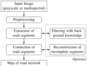
The proposed method is made of two main steps: extraction and connection of road segments. Robustness to false positives and negatives is ensured through two additional steps: filtering with background knowledge and reconstruction of incomplete segments, respectively. To address various kinds of input data (i.e., grayscale, color or multispectral images), a preprocessing step is also included. Figure 1 shows the overall flowchart.
For the sake of illustration, we provide in Fig. 2 two sam-ple images, and for each of them the intermediate results (after extraction and connection of road segments) as well as the re-sulting road network map.
Input Image (grayscale or multispectral)
Preprocessing
Map of road network Extraction of road segments
Connection of road segments
Filtering with back-ground knowledge
Reconstruction of incomplete segments
Optional
Fig. 1. Flowchart of the proposed method.
(a) (b)
(c) (d)
(a) (b)
(c) (d)
Fig. 2. Illustration of the main steps of our road extraction method: (a) input image extracted from a Quickbird image c copyright Digitalglobe 2008 (top) and from a Pl´eiades image c CNES 2012, Distribution Airbus DS (bottom), (b) extraction (in dark) of road segments and (c) connection through region-based path closing, and (d) final result after thresholding.
2.1. Preprocessing
The morphological operators involved in the overall process are applied on grayscale images, assuming that the road net-work is made of rather dark pixels in such images. This is usu-ally the case with asphalt roads observed from panchromatic images. But roads can be made of other material (e.g., con-crete or lightly colored rocks), and can be extracted from more informative data such as color or multispectral images.
Thus, the goal of the preprocessing step is to convert the in-put data f : E → T , with E ⊂ Z2the image grid and T ⊂ Rn the initial n-d value space, into a grayscale image g : E → V
(with V ⊂ R, e.g., V = [0, 255]) where road pixels are darker than the background. If no additional information is avail-able, the multiple input channels are merged to build a unique grayscale image, leading to an appropriate representation for asphalt roads. Otherwise, prior knowledge is used to derive a more accurate grayscale image to be further processed.
If the colors or spectral values of some n road materials are known (Herold and Roberts, 2005) and noted {c1, . . . , cn}, we compute a distance map where each pixel p is assigned the dis-tance from its spectral signature f (p) to the closest road color c (e.g., asphalt and concrete colors), i.e., g(p)= minid( f (p), ci), with d a predefined distance metric. Pixels that are made of the same material as roads are thus assigned very low values.
If training samples are available, we can also rely on a super-vised classification procedure. We consider two classes (road c and non-road c0) and compute membership probabilities m for each pixel p, i.e., mc(p) and mc0(p). Pixels that are most likely
to belong to roads (i.e., high mc) are assigned low values, e.g., with the measure g(p)= 1 − mc(p)= mc0(p).
In case no prior knowledge of road materials is available but multispectral images are given, vegetation can be discarded by computing the NDVI feature (normalized difference vegetation index, computed as (NIR − R)/(NIR+ R) with NIR and R de-noting respectively the near infrared and visible red bands) and masking the high NDVI values indicating vegetation areas.
Let us note that other transformations might be involved in case of specific visible content of road materials, e.g., tex-tured rock roads would require to compute texture features from which adequate gray values can be extracted. Such a strategy would allow limiting the large standard deviation of pixel val-ues that may occur.
All these various strategies aim to deliver a grayscale image that will be the input for the next steps.
2.2. Extraction of road segments
As already recalled, existing methods for road extrac-tion from remote sensing data usually operate at the pixel scale. However, recent sensors providing very high (spa-tial) resolution images (or VHR images) call for a higher level of analysis, similarly to the object-based image analysis paradigm (Blaschke, 2010). Indeed, the pixel scale both re-quires a high volume of data to be processed (thus preventing scalability) and is not well adapted to the very high spatial res-olution for which road width varies from 10 to 100 pixels. We address these two issues by introducing a segment extraction step, the goal of which is to change the analysis scale from pix-els to regions, or in other words from the image support E to the set of segments S.. Conversely to existing approaches re-lying on superpixels (Wegner et al., 2015) or regions produced by a segmentation (Long and Zhao, 2005), here the regions are identified within the image as possible road segments. We rely here on the assumption that a road segment corresponds to a rectangular area of relative homogeneous content.
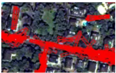
The extraction of road segments is then achieved through a probing step. It requires the definition of a rectangular template of predefined size (height and width), that is a priori defined based on the spatial resolution of the image to be processed
Fig. 3. Illustration of overlap among detected road segments (shown with red borders) to be corrected with the maximal overlapping ratio threshold.
(and is thus directly related to the visual appearance of roads in the image). The template is used as a sliding window when scanning the image. For each pixel, the template leads to the identification of its neighbors, all being compared with the pixel under analysis. From this comparison is computed the ratio of similar pixels within the template. If this ratio is higher than a predefined threshold, we consider that a possible road segment is present. Pixels are considered similar if their values are rel-atively close, i.e., within a predefined range. More formally, given a pixel location p, a new segment S will be extracted if
( card(p ∼ q) card(q) ≥ Tsim q ∈ N(p) ) ,
with N(p) the neighborhood of p defined by the sliding win-dow, T a given ratio threshold, and p ∼ q the similarity relation between a pixel p and its neighbor q. The similarity relation will be further discussed in Sec. 3.2. The grayscale value g(p) is transferred to the segment S built from p through a new im-age of segments defined as h : S → V : S 7→ h(S ).
Despite leading to efficient further processing of road seg-ments (instead of individual pixels), this probing step also comes with a significant computational cost. Indeed, it requires to analyze the full neighborhood of each single pixel. Such a neighborhood can be sampled, considering only a certain per-centage of the pixels in the comparison process (thus using N0 ⊆ N . As it will be demonstrated in the experiments, this allows greatly decreasing the computational cost without loss in detection accuracy. Let us observe that such an optimiza-tion would not have been possible if road segments were pro-duced from superpixels or with a standard segmentation tech-nique. Besides, geometrical properties of road segments are taken into account directly within the extraction step, with no need for post-processing beyond their connection.
While the proposed scheme allows for a great reduction in the number of elements to be subsequently processed, some ad-ditional heuristics can be involved to further increase the com-pression rate. Indeed, the overall computation cost is directly related to the number of road segments to be scanned by the path filtering operator. We thus include a constraint on the max-imal overlapping ratio between extracted segments. In other words, a segment is kept as long as its overlapping surface with existing segments is lower than a given ratio, or in other words if it brings a given amount of new content in the detected im-age. Let us note that such a strategy is sensitive to ordering is-sues, first extracted segments being given a higher importance in the selection process. A careful analysis of this parameter will be given in Sec. 3. Figure 3 illustrates the possible
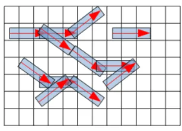
over-Fig. 4. Data structure used to store the set of segments.
lap between detected segments and the need for some overlap checking procedure as the one proposed here.
Besides, the shape of road segments can be dynamically ad-justed to fit as best as possible actual roads. To do so, we con-sider variable widths for the roads segments. The neighborhood analysis described above assumes a predefined road width. If, for a given pixel, a segment is found, the neighborhood is it-eratively extended (by step of 2 pixels) to consider larger road segment width. This allows considering roads with changing width (e.g., from 3 to 4 lanes and back).
2.3. Connection of road segments
Once road segments have been identified, they are used as the elementary units of the image for further processing. While the set of segments is formally defined as S and associated gray values stored in the image h, in practice we store them in a ded-icated grid structure, namely a matrix allowing to access both starting and ending segments at a given image location. Each cell contains two lists of segments, respectively starting and ending at the coordinates indicated by the cell indices. Since the number of segments is much smaller than the number of image pixels, the matrix is indeed sparse. Figure 4 illustrate the data proposed structure, showing that one segment ends in (3, 2) while two segments start from this cell.
Inspired by the work from Valero et al. (2010), we consider here path closing (Talbot and Appleton, 2007), a morphological filter able to extract curvilinear structures. Indeed, it is possible to distinguish between a road (i.e., a chain of segments with sig-nificant length) and a building (an unordered set of segments) while these objects can share the same spectral properties.
Original algorithms for path filtering from Talbot and Apple-ton (2007) require some adaptation to process segments instead of pixels. Paths were originally built by linking neighboring pixels depending on their graylevel and following a given di-rection. Based on our grid data structure, we define here the neighborhood N of a given segment S as the set of all segments overlapping S and having a grayscale lower or equal to the one of S , i.e. N(S )= {S0∈ S | S ∩ S0, ∅ and h(S0) ≤ h(S )}. To ensure robustness, we modify this definition by also consider-ing segments relatively close to S (distance between segments lower than a threshold), and with a similar orientation (orien-tation difference lower than a threshold). Several strategies can be used to connect these non-overlapping segments (see Fig. 5): i) two segments are connected if the end of the first segment is within the neighborhood of the beginning of the second seg-ment (Fig. 5 left); ii) the connection can also rely on a more advanced definition of the junction area, i.e., any predefined
r1
r2
r1
r2
Fig. 5. The two possible strategies to connect successive road segments: using a disc of predefined radius (left) or any predefined shape (right). The latter one allows for greater flexibility and avoids misconnections.
Fig. 6. Illustration of path length computation. For each segment, the length of the longest path it belongs to is shown.
shape instead of a single disc of a given radius (Fig. 5 right). The second strategy is more flexible and allows for a more pre-cise definition of the connection process. To illustrate, the sec-ond strategy is able to avoid misconnection of segments from the configuration given in the left part of Fig. 5.
We consider here a morphological path closing φ, whose aim is to identify long dark paths, while all other structures will be brightened (the dual operator, path opening γ, should be used if the road network is represented by bright pixels over a dark background). The overall algorithm is applied iteratively on graylevels, from the lowest (black) to the highest (white) lev-els. For each graylevel or value v, paths are built from seg-ments with graylevel lower or equal to v. Each segment S is set to graylevel v if it belongs to a path whose length is higher than a threshold. Thus, it will be kept unchanged if it is possible to build a path of significant length from its graylevel. Otherwise, it will necessarily belong to a path of higher graylevel, and thus will have its graylevel set accordingly. The path closing opera-tor adapted for segments is thus a transform φ : VS→ VSthat operates on an image of segments (or mapping form the space of segments S to the value space V):
φ(h(S )) = min(v)
∃ P, length(P) ≥ Tpath, S ∈ P,
∀S0∈ P, h(S0) ≤ v. Algorithm 1 provides a formal definition of the path closing op-erator when applied on segments. Depending on the scanning order (from image top to bottom (North to South), left to right (West to East), or conversely), the northern/southern segments are the segments with ending/starting coordinates in the neigh-borhood of the considered segment. The list L is thus obtained through the analysis of the grid data structure (Fig. 4). For the sake of illustration, we provide in Fig. 6 the length of the paths built from segments stored in the data structure shown in Fig. 4. The road segments contained in the filtered image have their
Algorithm 1: Path Closing on Segments.
// Parameters
lmin: minimal path length for roads // Preprocessing and extraction of segments
L: list of segments sorted by row N/S and column W/E // Fields of segment structure
seg.active : active flag used in the algorithm seg.value : segment value (graylevel) after detection seg.length : segment length (in pixels)
seg.fvalue : final value of the segment (after closing) seg.lup : maximal length for North path
seg.ldown : maximal length for South path // Initialization seg.active=false seg.fvalue=null seg.lup=0 seg.ldown=0 // Processing
forall the values V from black to white do // First Scan (list N/S and W/E, update lup) activate segments from list L when seg.value= V forall the all active segments S in list L do
forall the attached northern segments aSeg do S.lup ← max (S.lup, aSeg.lup+ aSeg.length) end
if S.lup is updated AND S.fvalue= null then if S.lup+ S.ldown + S.length ≥ lmin then
S.fvalue ← V end
end
if S.lup is updated OR S.value= V then forall the southern rectangles aSeg do
if aSeg.value ≤ V then aSeg.active ← true end end end S.active ← false end
// Second Scan (with inverted list S/N and E/W)
// Third and Fourth Scans, updating seg.ldown and reactivating northern segments instead of southern ones
end
graylevels brightened depending on the size of the longest path they belong to. It is then straightforward to produce the final road network map with a simple thresholding.
2.4. Filtering with background knowledge
Accuracy of the road network map directly relies on the quality of road segments extracted in the first step. Among these segments, a significant subset corresponds to large and homogeneous areas (e.g., parking lots, courts, fields, etc.) and leads to false positives. We propose to take into account back-ground knowledge for a more accurate identification of road segments. We thus follow the principle of the Hit-or-Miss Transform (HMT) that led to the successful design of template matching solutions for a wide range of problems, including in remote sensing (Lef`evre et al., 2014). Assuming that roads can be distinguished from other areas by their width, we modify the first step to take into account both a foreground rectangu-lar template and a composite background template. The latter
Fig. 7. HMT ability to deal with background knowledge and distinguish between actual road segments (yellow) and outliers (red). Foreground and background are respectively probed with the central and side rectangles.
is made of two parallel rectangular areas located on each side of the foreground template. Distance between these templates and the foreground one is set depending on the expected road width and its possible variation (e.g., varying number of lanes). The pixels not contained in the foreground nor the background templates (i.e., in-between area) corresponds to an uncertainty zone, and are not involved in the template matching process. The probing now operates on two criteria: all pixels covered by the foreground template shall have a similar value to the central pixel, i.e., foreground color, while all pixels covered by the background template shall have a different value to the cen-tral pixel, i.e., background color. Let us remark that the ratios of similar pixels for the foreground and background template have to differ, since the uniformity imposed on road segments is not valid anymore when dealing with background (that can be made of any material). The proposed filtering with back-ground knowledge step leads to the extraction of a segment S from pixel location p if both following conditions hold:
( card(p ∼ q) card(q) ≥ Tsim-fg q ∈ Nf g(p), ) , ( card(p q) card(q) ≥ Tsim-bg q ∈ Nbg(p) ) ,
with Nf gand Tsim-fg (resp. Nbg and Tsim-bg) the neighborhood defined by foreground (resp. background) template and its re-lated ratio threshold.
Figure 7 shows this step allows distinguishing between ac-tual road segments and regions that compose large pieces of the same material (e.g., asphalt, concrete) but are not roads. 2.5. Reconstruction of incomplete segments
While the previous step aims to remove false positives, it is also necessary to remove false negatives. Indeed, some roads might not be completely detected due to a partial occlusion (e.g., by trees, shadow, cars, pedestrian crossing, etc.) of road segments, leading to their heterogeneous content and a subse-quent missed detection. This in turn results in roads of insu ffi-cient length, discarded by the path closing process.
Similarly to Talbot and Appleton (2007), we also rely on in-complete path filtering to deal with missing elements. Let us recall that here, elements are segments instead of pixels. A scanning process is started for each road extremity. It tries to fill with a small set of successive segments the possible gap
Fig. 8. Illustration of path length computation (from top to bottom): a set of segments with their path length, the candidate segments to complete existing paths (only segments located at extremities of existing paths are considered), and finally the selected segments (connecting two paths) with path length recomputed.
Fig. 9. Illustration of the ability of incomplete path filtering to reconnect disconnected road segments: initial segments are given in red, added seg-ments are in blue, thus resulting in length updating in the path filtering process that is finally able to return new segments (in green).
between the current road and another one. To ensure coher-ence between the added segments and the original ones, and to avoid the inclusion of outliers (e.g., a building located between two roads), the connecting segments shall share some common properties. Here we rely on the same criteria than in the path closing step, but using some lowered constraints (thresholds). This reconstruction process is included in the general path clos-ing step, thus enablclos-ing to connect road segments even in pres-ence of missing segments.
For the sake of illustration, we provide in Fig. 8 an exam-ple of path comexam-pletion, where the candidate segments located at path extremities are used to connect two paths, leading to a further path length updating step.
Figure 9 shows this step allows reconnecting segments that were initially unconnected (in red), relying on both filling seg-ments (in blue) and new segseg-ments (in green) extracted follow-ing the update of the path length. While present in the set of segments extracted after the first step of the method, such new segments were initially discarded since they were not belong-ing to a path of sufficient length. The proposed incomplete path filtering procedure prevents discarding such segments.
3. Experiments
Our method has been assessed on various satellite images. We provide here some comparative results with the state-of-the-art, as well as some analysis and discussion of the different parameters involved in the different steps of our method. 3.1. Datasets and evaluation measures
To assess our contribution, we have performed a series of ex-periments on various satellite images. For the sake of compar-ison, we will consider here Quickbird images and show results obtained both on a grayscale image of 420 × 300 pixels used by Valero et al. (2010), and on a multispectral image of 2832×2772 pixels from Strasbourg, France. The latter has been converted to grayscale and is associated with some validation data pro-vided by French Geographic Institute IGN. We also assess our method on some Ikonos images from an almost 10 years old dataset (Mayer et al., 2006). As observed in results reported in recent works (e.g., Shi et al. (2014)), this dataset can still be considered as a reference, and the last years have not seen sig-nificant advances of the state-of-the-art. Comparative results as well as quantitative measurements will be provided in Sec. 3.3. Evaluation is performed using standard measures. We con-sider here the criteria proposed by Wiedemmann et al. (1998) and still commonly adopted e.g., by Bae et al. (2015): com-pleteness (or recall, sensitivity), correctness (or precision), as well as a quality score inspired from the accuracy measure. The latter is defined using T P, FP, FN (respectively denoting true positives, false positives, and false negatives) by the ratio T P/(T P + FP + FN). It is very similar to the standard accuracy measure, the only difference being the lack of T N (true nega-tives) in the denominator, in order to accommodate with the un-balanced classes (roads vs. non-roads). As indicated by Mayer et al. (2006), practical usefulness of road network extraction methods requires completeness and correctness scores above 0.6 and 0.75, respectively. Let us recall that they are respec-tively computed as ratios T P/(T P+ FN) and T P/(T P + FP). Furthermore, we also use the F1-score (harmonic mean of com-pleteness and correctness, i.e., (2T P)/(2T P+ FP + FN)) when considering the IKONOS dataset, to ease fair comparison with the state-of-the-art results achieved on this dataset.
3.2. Parameter settings
The method proposed in this paper relies on a number of parameters that have been set empirically from image proper-ties (e.g., spatial resolution, contrast). In the experiments that will be reported in the comparative evaluation (Strasbourg im-age), we have used the following settings. Road segments have width of 5 pixels, and height of 45 pixels. Segments are de-tected in all orientations with an angular step of 5◦. Maximal orientation change and maximal distance between segments are respectively set to 30◦and 5 pixels. Pixels are considered sim-ilar if their graylevels are equal ±5%. The rate of simsim-ilar pix-els within a segment is set to 100% (all pixpix-els shall be similar). Background knowledge requires the definition of an uncertainty zone in the HMT process. It has been set here equals to road width (5 pixels). The ratio of similar pixels within the back-ground template is set to 20 % since less assumptions can be
(a) (b) (c) (d)
Fig. 10. Road network extraction, easy dataset: original image from (Valero et al., 2010) (a) and results from OTB (b), Valero et al. (c), and our method (d).
Table 1. Comparison of road network extractors, easy dataset. Method Completeness Correctness Quality
OTB 0.63 0.70 0.50
Valero et al. 0.95 0.78 0.76 Proposed 0.93 0.85 0.81
made on the uniformity of the background (i.e., non road) ar-eas. Reconstruction fills gaps of length once or twice the length of segments (i.e., 45 or 90 pixels). A path is considered as a road if it contains at least 5 successive segments (ca. 250 pix-els). Finally, pixels from the filtered image are kept in the road network map if their graylevel is lower to 128. Since we con-sider here asphalt roads, the final map contains the dark half of the filtered image, while the other objects are made of pix-els brightened by the region-based morphological filtering. But as described in Sec. 2.1, the preprocessing allows dealing with other contexts and images.
Since parameters have been set here empirically, we provided in Sec. 3.5 some analysis of their impact on the end-results. Their automatization is left for future work. Indeed, the pa-rameters greatly depend on the image properties but also on the kind of road network considered, since the latter may vary con-siderably from one country to the other, and even within a given country (urban versus rural areas).
3.3. Accuracy evaluation
We compare our method with two representative tech-niques from the state-of-the-art: the road extraction algorithm available in OTB (CNES ORFEO Tool Box, http://www. orfeo-toolbox.org/otb) and the method from Valero et al. (2010) that motivated our work. The latter has been here initial-ized manually with the parameters leading to the best results.
We first consider the easiest dataset already suggested in (Valero et al., 2010). We can observe in Fig. 10 that both our method and Valero et al. (2010) provide similar results, bet-ter than with OTB which does not rely on paths. A quantita-tive analysis is provided in Tab. 1, confirming the conclusions driven from visual analysis.
A second and more challenging experiment has been per-formed with the Strasbourg image. We can see in Fig. 11 (a subset of the original image for better visualization) that roads have a very similar color to the background. While such a dif-ficult scenario cannot be tackled by Valero et al. (2010) (nor by the OTB method which is unable to analyze such a complex im-age), our method (with all steps from Fig. 1) is able to extract
(a) (b) (c)
Fig. 11. Road network extraction, challenging dataset: RGB composition (a) of the original image c Digitalglobe 2008, and results from Valero et al. (b) and our method (c).
Table 2. Comparison of road network extractors, challenging dataset. Method Completeness Correctness Quality Baseline 0.68 0.80 0.58 Baseline+ Filtering 0.70 0.82 0.61 Reconstruction 0.69 0.81 0.60 Reconstruction+ Filtering 0.71 0.83 0.62
the most important elements of the road network. We clearly observe the relevance of mapping road segments by rectangular areas, making possible to distinguish between road segments and neighboring pixels of similar color or graylevel.
Once roads have been extracted, the availability of some ref-erence data provided by IGN allows us performing a quantita-tive evaluation. Only a part of the Strasbourg image is available with some ground truth (Fig. 11(a), 1000 × 1000 pixels) and leads to quantitative evaluation. Tab. 2 gives the results ob-tained with our baseline method, as well as alternative steps to improve robustness to false positives/negatives. We can quanti-tatively assess the relevance of these options.
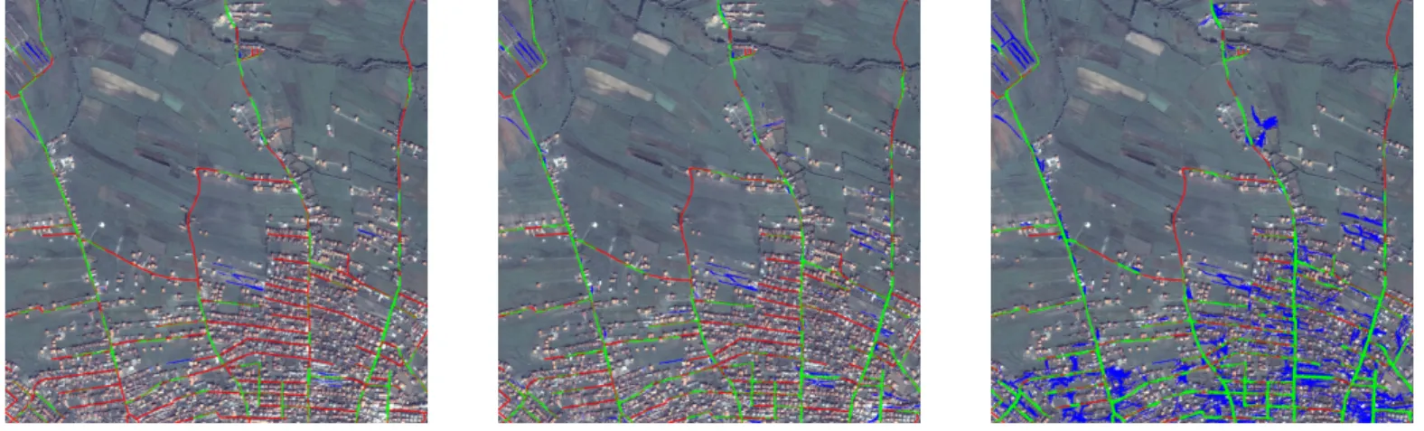
Finally, we also report accuracy evaluation on the IKONOS dataset used in the comparative evaluation performed by Mayer et al. (2006). Results obtained on the Ikonos1-Sub1 image are given in Fig. 12, using the same color code as in the original paper, and with different settings favoring completeness, cor-rectness, or both. Indeed, parameter settings can be achieved to increase completeness or correctness, as shown in Tab. 3, lead-ing to similar overall accuracy scores (measured here with the F1 Score). Finding a compromise between completeness and correctness (thus trying to lower both false positives and false negatives) allows reaching a higher level of overall quality, as shown in Tab. 3. We can see on the last line of the table that the proposed settings is not far to meet the requirements for practical usefulness (completeness of 0.6, correctness of 0.75) defined by Mayer et al. (2006) on this challenging dataset. Let us recall that F1 scores reported in the initial study were vary-ing between 0.37 and 0.57, and that even recent methods such as (Shi et al., 2014) hardly tackle this dataset.
3.4. Performance evaluation
Beyond a major improvement in detection accuracy, the pro-posed region-based morphological scheme also allows a sig-nificant decrease of computation time. We compare here our method with the initial work of Valero et al., for which we have realized a Java-based implementation based on the C++ code
Fig. 12. Illustration of road network extraction with correctness preferred (left), completeness preferred (right), or compromise between both objectives (center). True positives, false negatives and false positives are respectively displayed in green, red, and blue.
Table 3. Quantitative evaluation on the IKONOS dataset, various settings favoring completeness, correctness, or both.
Settings Completeness Correctness F1 Score
Low FN 0.71 0.42 0.53
Low FP 0.42 0.81 0.56
Low FN and FP 0.60 0.69 0.64 Shi et al. (2014) 0.34 0.63 0.44
provided by the authors (so ensuring a fair level of optimiza-tion). As far as our method is concerned, it comes with a moder-ate level of optimization (single-threaded, with all optimization tricks described in the previous sections). Using a similar cod-ing language and operatcod-ing environment allows for more objec-tive comparison. Furthermore, both methods are characterized with a similar computational complexity, since both rely on the principles of the path opening operator. There is however a ma-jor difference, that lies in the kind of elements to be processed (segments instead of pixels).
Measures obtained with the full Strasbourg image are re-ported in Tab. 4 (using a standard workstation, with a i5 2.5 GHz CPU and 8 GB RAM). Let us observe that our method requires 22 seconds to extract road segments, which lowers the efficiency gain if no reconstruction is performed. However, pro-cessing regions instead of pixels leads to a major improvement in efficiency as soon as a reconstruction step is involved. More-over, the complexity increases only slightly when considering gaps of higher length (1 or 2 segments, i.e., ca. 50 or 100 pix-els). Let us note that these results shall be considered carefully since optimization was only moderate.
Most of the papers introducing new road detection methods do not provide indications of computation time. Nevertheless, our method seems very competitive w.r.t. the state-of-the-art, e.g., more than one hour is required by Ouled Sghaier and Lep-age (2015) to process a 2048 × 2048 imLep-age.
As far as the memory cost is concerned, we have measured the memory footprint with a profiling tool (namely jVisualVM). The Java user heap was 1.86 GB for Valero et al, while only 0.95 GB with our algorithm, for processing the Strasbourg im-age (31 MB). Both methods were performing an incomplete path opening. Let us recall that these values were obtained
Table 4. Comparison of processing times (in seconds). Method Reconstruction CPU Time Valero et al. no 98 Valero et al. 1 pixel 310 Valero et al. 2 pixels 720
Proposed no 84
Proposed 1 segment 117 Proposed 2 segments 119
without specific optimization, and the structure we are using (a sparse matrix to store two lists of segment extremities) con-tributes to a gain in CPU cost w.r.t. a linked list structure, but at an additional memory cost. Nevertheless, we can observe a sig-nificant gain in terms of memory cost, that is easily explained by the change of representation: while the original work from Valero et al. was operating on pixels, the proposed method is processing road segments, i.e., objects that are far less numer-ous than image pixels.
3.5. Discussion on heuristics and parameters
Several heuristics related to the extraction of segments were introduced in Sec. 2.2. We report here some experimental re-sults obtained when conducting further analysis to understand how they behave in the overall process.
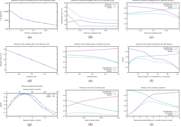
We first study how the overlapping ratio threshold influences the number of extracted segments, and subsequently the overall computation time as well as the accuracy of the end results. We consider various ratios from 1 (no overlapping constraint, over-lapping allowed until 100%) to 0 (strict overover-lapping constraint, no overlapping allowed). The results are given in first line of Fig. 13 and show the great effect of this constrained selection procedure on the number of extracted segments that composed the space on which the path filtering process operates. We can observe that reducing the number of segments leads to a very significant gain in performance, while keeping satisfying accu-racy levels (e.g., keeping a segment only it it brings 75% of new content, i.e., maximal overlapping ratio lower than 25%, reduces by a factor of 35 the number of segments, by 5 the path filtering time and by 2.5 the overall time, for a 20 points loss in completeness and no loss in overall quality. Conversely, a slight
gain in quality can be observed. It is probably due to the fact that the unconstrained scenario extracts some erroneous rectan-gles located on road borders (partly inside, partly outside the actual road). Such a situation is alleviated with the overlapping constraint that force extracted rectangles to be aligned (on the road direction). But this gain is lowered when the overlapping ratio becomes too low, since there is then not enough remain-ing road segments for the filterremain-ing step. Considerremain-ing a maximal overlapping ratio of 50% allows reaching a quality level of 0.59 (i.e., gain of 4.5 points), for only an half of the initial CPU cost. Another optimization consists in considering only a certain percentage of the pixels in the neighborhood when checking if a segment has to be selected or filtered out. Figs. 13(d) and (e) show that this sampling procedure leads to a significant de-crease in computation time for the detection step (d), with no prohibitive loss in accuracy up to a certain sampling ratio (e). Indeed, the method is able to provide results of similar quality when considering only 50% of the pixels.
We have also studied how the dynamic width adjustment in-fluences the quality of the end results. However, on the Stras-bourg image considered so far, the observed differences in qual-ity score were not considered as significant (lower than 1%). Similarly, using an advanced neighborhood configuration to connect successive segments has not led to major improvement, since the gain in correctness has been counterbalanced by a loss in completeness, resulting in an overall gain in quality of ca. 1%. We are convinced that conducting additional experi-ments on other datasets will be helpful in assessing the rele-vance of these various heuristics.
The overall process relies both on extraction and connection of road segments, whose parameters’ influence are studied in the remaining plots of Fig. 13. The first step is parametrized by the dimensions and heterogeneity of the road segments to be extracted. Fig. 13(g) shows how dimensions influence the over-all result. When dimensions are close to 1, the region-based path filtering will act similarly as the standard one (i.e., pixel-wise) and keep small areas located along the road. Conversely, high values for segment length and width will prevent selecting curved and narrowed roads, respectively. Appropriate dimen-sions have to be set depending on the visual appearance of roads in the processed image. We can observe that working with seg-ments of elongation ratio around 1:10 (i.e., 50 × 5 for length × width) as basic units for the morphological path filtering op-erator used in the second stage leads to the best results. Road segments are defined by their dimension but also by their con-tent. More precisely, a road segment is extracted if it contains a significant ratio of similar pixels in a rectangular neighbor-hood (see Sec. 2.2). Thus, Figs. 13(h) and (i) show respectively the effect of the ratio parameter and similarity constraint. We can observe that accepting 1% of outliers leads to better results, while higher values tend to lower the overall quality. Further-more, a tolerance in terms of graylevels within the segment is required to achieve satisfying results. Defining two pixels as similar if the difference between their graylevels is not lower than 5 or 6 % of the graylevel range provides the best results. Let us note that a very low difference (e.g., 0, all pixels have to be strictly equal; or 1, all pixels should share the value of the
centered pixel ±1%) prevent detecting any road segment. The second step, namely connection of road segments, con-sists in a morphological path filter. It relies on an additional parameter defining the minimal path length or the number of successive segments that a path should contain to remain af-ter the filaf-tering step (similarly to the path length used with the standard path filtering operator). As shown on the Fig. 13(f), this filtering is mandatory to eliminate false positives (resulting in gain of 15 points in correctness), and best results where ob-tained with a threshold value of 9. Let us note that a length of 9 segments is equal to 225 pixels (each segment being 25 pixels long in the settings used for this figure), and the processed im-age is here 1200 × 800 pixels. Higher threshold values result in discarding small roads, leading to a loss in detection quality. 3.6. Requirements for better spatial resolution
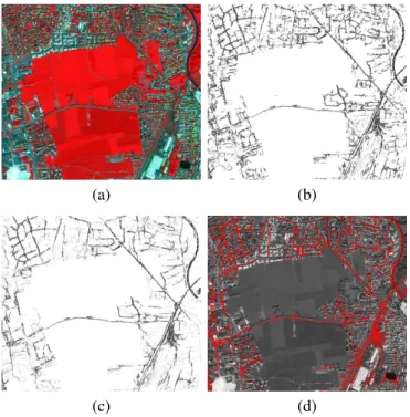
Results provided so far were promising and show how our method outperforms the state-of-the-art. Nevertheless, we have also observed its limitations in some specific cases, e.g., when road segments were very narrow (while our method is assum-ing a minimal width). As illustrated in Fig. 14, some road seg-ments are then not extracted if only graylevels are used. Indeed, on the image given in the aforementioned figure, the method achieved low recognition rates (0.34 for completeness, 0.44 for correctness), below expected standards defined by Mayer et al. (2006). This demonstrates the need for relying on additional or updated data when detection is particularly challenging. Let us note that detection is eased with new sensors such as Pl´eiades that come with a higher spatial resolution (50cm/pixel for the Pl´eiades color image vs 2.4m/pixel for the Quickbird multi-spectral image). To illustrate, Fig. 2 (bottom) used in Sec. 2 shows how road segments are extracted from a grayscale image of Strasbourg, and with the same setup as Fig. 14. Recognition rates climb up to 0.79 for completeness, 0.69 for correctness, leading to a global quality score of 0.58.
Experiments with Pl´eiades images have been conducted with two other geographical areas of France, namely St-Jean-de-Luz and Lorient, and results are given in Fig. 15. While in the first case the road network is accurately extracted from residential areas, the second one is much more challenging. Roads do not have a constant spectral value especially due to shadows, and can be sometimes barely visible. The proposed method is able to extract only a (significant) part of the road network. It can then be used as a very efficient deterministic initialization of more complex probabilistic strategies.
4. Conclusion
Extraction of roads from aerial or satellite images allows maintaining an up-to-date map of road networks. While ex-plored for decades, automatic road extraction remains challeng-ing. Very high spatial resolution sensors provide more details that should ease recognition techniques, but also bring a higher data volume and lead to visual appearance of roads made of elongated structures with a width higher than a single pixel. In this paper, we address these issues by introducing new region-based morphological operators. We first map an input image
1000 10000 100000 1x10⁶ 0 0.25 0.5 0.75 1 # of segments
Maximal overlapping ratio
Influence of maximal overlapping ratio on the compression effect
0 10 20 30 40 50 60 0 0.25 0.5 0.75 1
computation time (in s)
Maximal overlapping ratio
Influence of maximal overlapping ratio on the computation time extraction connection overall 0 0.2 0.4 0.6 0.8 1 0 0.25 0.5 0.75 1
Maximal overlapping ratio
Influence of maximal overlapping ratio on detection accuracy Completeness Correctness Quality (a) (b) (c) 6 8 10 12 14 0.2 0.4 0.6 0.8 1
detection time (in s)
Sampling ratio
Influence of the sampling ratio on the detection time
0 0.2 0.4 0.6 0.8 1 0.2 0.4 0.6 0.8 1 Sampling ratio
Influence of the sampling ratio on detection accuracy
Completeness Correctness Quality 0 0.2 0.4 0.6 0.8 1 10 20 30 40 50 Quality
Minimal length in # of segments (i.e. 25 pixels) Influence of the length threshold for the path filtering
Completeness Correctness Quality (d) (e) (f) 0 0.1 0.2 0.3 0.4 0.5 0.6 0 4 8 12 16 0 40 80 120 160 Quality
Segment length (in pixels) Influence of segment dimension
Segment width (in pixels) width length 0.5 0.6 0.7 0.8 0.9 1 0.97 0.98 0.99 1
Ratio of similar pixels Influence of the radio of similar pixels
Completeness Correctness Quality 0 0.2 0.4 0.6 0.8 1 2 3 4 5 6 7 8 9 10
Maximal greyscale difference to consider pixels as similar Influence of the similarity constraint
Completeness Correctness Quality
(g) (h) (i)
Fig. 13. Influence of parameters settings: maximal overlapping ratio effect on the number of extracted segments (a), the overall complexity (b) and quality of the full detection process (c); sampling ratio effect on the complexity of the detection step (d) and the quality of the full detection process (e); observed quality measures for different values of the road segment connection parameter (f) and of the road segment extraction parameters: segment dimensions (g), ratio of similar pixels (h), and graylevel difference to define similarity (i).
into a set of road segments which become the elementary im-age units. Such elements are then processed with an (incom-plete) path closing algorithm, the aim of which is to emphasize segments belonging to the road network.
Experiments conducted on various satellite images demon-strate how our method outperforms existing solution using path closing at the pixel scale (Valero et al., 2010), both in terms of accuracy and efficiency. Results obtained with very high spatial resolution images (such as the ones provided by the Pl´eiades sensor) show that our method achieves automatic road extraction with a satisfying level of accuracy. Nevertheless, our method is not yet able to address aerial datasets such as the one provided by the ISPRS Test Project on Urban Classification and 3D Building Reconstruction (Rottensteiner et al., 2012). We have indeed observed that shadows are playing a crucial role in this dataset, and are making roads appearing as disconnected paths (and thus are calling for a specific shadow processing to address such artefacts).
Among future research directions, we believe the color/spectral information could be addressed in a better way, through color/multispectral morphological operators
(Ap-toula and Lef`evre, 2007) instead of the conversion to graylevels used as preprocessing. Beyond color, texture information can also be taken into account. Furthermore, the proposed approach being only deterministic, it could be combined with probabilistic modeling or refinement of road segments. Finally, improved path filtering algorithms have been recently proposed (Cokelaer et al., 2012; Morard et al., 2014) and could also benefit to our method (if adapted to the region scale).
Acknowledgments
The authors would like to thank A. Puissant from LIVE UMR CNRS 7362 (University of Strasbourg) for providing the geometrically corrected images of Strasbourg (Quickbird and Pl´eiades sensors), and H. Mayer from Bundeswehr University Munich for providing the IKONOS dataset (Mayer et al., 2006). IKONOS images are c Bundeswehr Geoinformation Office (AGeoBw), Euskirchen, Germany. This work has been sup-ported by the French Agence Nationale de la Recherche (ANR) under reference ANR-13-JS02-0005-01 (Asterix project).
(a) (b)
(c) (d)
Fig. 14. Road network extraction with a very challenging dataset with nar-row road segments: (a) RGB composition of the original Quickbird image – Strasbourg North area c Digitalglobe 2008, outputs of the road segment (b) detection and (c) connection steps, and (d) final map superimposed on the panchromatic processed image.
References
Aptoula, E., Lef`evre, S., 2007. A comparative study on multivariate mathemat-ical morphology. Pattern Recognition 40, 2914–2929.
Bae, Y., Lee, W., Choi, Y., Jeon, Y., Ra, J., 2015. Automatic road extraction from remote sensing images based on a normalized second derivative map. IEEE Geoscience and Remote Sensing Letters 12, 1858–1862.
Bajcsy, R., Tavakoli, M., 1976. Computer recognition of roads from satellite pictures. IEEE Transactions on Systems, Man, and Cybernetics 6, 623–637. Besbes, O., Benazza-Benyahia, A., 2014. Joint road network extraction from a set of high resolution satellite images, in: European Signal Processing Conference (EUSIPCO), pp. 2190–2194.
Blaschke, T., 2010. Object based image analysis for remote sensing. ISPRS Journal of Photogrammetry and Remote Sensing 65, 2–10.
Cokelaer, F., Talbot, H., Chanussot, J., 2012. Efficient robust d-dimensional path operators. IEEE Journal of Selected Topics in Signal Processing 6, 830–839.
Courtrai, L., Lef`evre, S., 2014. Road network extraction from remote sens-ing ussens-ing region-based mathematical morphology, in: IAPR Workshop on Pattern Recognition in Remote Sensing (PRRS).
Gaetano, R., Zerubia, J., Scarpa, G., Poggi, G., 2011. Morphological road segmentation in urban areas from high resolution satellite images, in: Inter-national Conference on Digital Signal Processing, pp. 1–8.
G´eraud, T., Mouret, J., 2004. Fast road network extraction in satellite images using mathematical morphology and markov random fields. EURASIP Jour-nal on Applied SigJour-nal Processing 16, 2503–2514.
Herold, M., Roberts, D., 2005. Mapping asphalt road conditions with hyper-spectral remote sensing, in: International Symposium Remote Sensing of Urban Areas (URS), ISPRS.
Lef`evre, S., Aptoula, E., Perret, B., Weber, J., 2014. Morphological template matching in color images, in: Celbi, E., Smolka, B. (Eds.), Advances in Low-Level Color Image Processing. Springer. volume 11 of Lecture Notes in Computational Vision and Biomechanics, pp. 241–277. doi:10.1007/ 978-94-007-7584-8_8.
Long, H., Zhao, Z., 2005. Urban road extraction from high-resolution optical satellite images. International Journal of Remote Sensing 26, 4907–4921. Mayer, H., Hinz, S., Bacher, U., Baltsavias, E., 2006. A test of automatic road
(a) (b)
(c) (d)
Fig. 15. Road network extraction on sample Pleiades images: (a) original image of St-Jean-de-Luz c CNES 2013, Distribution Airbus DS and (b) extracted road network; (c) original image of Lorient c CNES 2012, Dis-tribution Airbus DS and (d) extracted road network.
extraction approaches, in: International Archives of the Photogrammetry, Remote Sensing and Spatial Information Sciences, pp. 209–214.
Mena, J., 2003. State of the art on automatic road extraction for {GIS} update: a novel classification. Pattern Recognition Letters 24, 3037–3058. Mnih, V., Hinton, G., 2010. Learning to detect roads in high-resolution aerial
images, in: European Conference on Computer Vision, pp. 210–223. Morard, V., Dokladal, P., Decenci`ere, E., 2014. Parsimonious path openings
and closings. IEEE Transactions on Image Processing 23, 1543–1555. Ouled Sghaier, M., Lepage, R., 2015. Road extraction from very high resolution
remote sensing optical images based on texture analysis and beamlet trans-form. Selected Topics in Applied Earth Observations and Remote Sensing, IEEE Journal of to appear, 1–13.
Rottensteiner, F., Sohn, G., Jung, J., Gerke, M., Baillard, C., Benitez, S., Bre-itkopf, U., 2012. The ISPRS benchmark in urban object classification and 3d building reconstruction. ISPRS Annals of Photogrammetry, Remote Sensing and Spatial Information Sciences I-3, 293–298.
Shi, W., Miao, Z., Debayle, J., 2014. An integrated method for urban main-road centerline extraction from optical remotely sensed imagery. IEEE Transac-tions on Geoscience and Remote Sensing 52, 3359–3372.
Sujatha, C., Selvathi, D., 2015. Connected component-based technique for automatic extraction of road centerline in high resolution satellite images. EURASIP Journal on Image and Video Processing 8, 1–16.
Talbot, H., Appleton, B., 2007. Efficient complete and incomplete path open-ings and closopen-ings. Image and Vision Computing 25, 416–425.
Unsalan, C., Sirmacek, B., 2012. Road network detection using probabilis-tic and graph theoreprobabilis-tical methods. IEEE Transactions on Geoscience and Remote Sensing 50, 4441–4453.
Valero, S., Chanussot, J., Benediktsson, J., Talbot, H., Waske, B., 2010. Ad-vanced directional mathematical morphology for the detection of the road network in very high resolution remote sensing images. Pattern Recognition Letters 31, 1120–1127.
Wang, J., Song, J., Chen, M., Yang, Z., 2015. Road network extraction: a neural-dynamic framework based on deep learning and a finite state ma-chine. International Journal of Remote Sensing 36, 3144–3169.
Wegner, J., Montoya-Zegarra, J., Schindler, K., 2015. Road networks as col-lections of minimum cost paths. ISPRS Journal of Photogrammetry and Remote Sensing 108, 128–137.
Wiedemmann, C., Heipke, C., Mayer, H., Jamet, O., 1998. Empirical evaluation of automatically extracted road axes, in: IEEE Computer Society Workshop on Empirical Evaluation Techniques in Computer Vision, pp. 172–187. Zhu, C., Shi, W., Pesaresi, M., Liu, L., Chen, X., King, B., 2005. The
recog-nition of road network from high-resolution satellite remotely sensed data using image morphological characteristics. International Journal of Remote Sensing 26, 5493–5508.