China's energy intensity and its determinants at the provincial level

(1)

CHINA'S ENERGY INTENSITY

AND ITS DETERMINANTS AT THE PROVINCIAL LEVEL

By

ARCIWES

Xin Zhang

Bachelor of Science in Electronics Engineering, Fudan University, 2003 Master of Science in Management, Ecole des Mines de Paris, 2006

Master of Science in Real Estate Development, Massachusetts Institute of Technology, 2008 Submitted to the Department of Civil and Environmental Engineering and Department of Urban Studies

and Planning in partial fulfillment of the requirements for the degrees of

MASSACHUSETTS INSTITUTE

Master of Science in Transportation OF TECHNOLOGY

Master of City Planning at the

_{JUL 10 2009}

MASSACHUSETTS INSTITUTE OF TECHNOLOGY

June 2009

LIBRARIES

The author hereby grants to MIT the permission to reproduce and to distribute publicly paper and electronic copies of the thesis document in whole or in part in any medium now known or hereafter

created.

Author

Department of Civil and Environmental Engineering Department of Urban Studies and Planning February 3, 2009 Certified by

Karen R. Polenske Professor of Regional Political Economy and Planning Thesis Supervisor

Certified by

Moshe Ben-Akiva Professor of Civil and Environmental Engineering

/ Thesis Reader

Accepted by

JgPph Ferreira

Chair, MCP Committee Department of Urban Studies and Planning

Accepted by

Chimn Coan •a~l ad St iantefnrG -...

(2)

(3)

CHINA'S ENERGY INTENSITY

AND ITS DETERMINANTS AT THE PROVINCIAL LEVEL By

Xin Zhang

Submitted to the Department of Civil and Environmental Engineering and Department of Urban Studies and Planning on February 3, 2009 in partial fulfillment of the requirements for the

degrees of

Master of Science in Transportation and Master of City Planning

Abstract

Energy intensity is defined as the amount of energy consumed per dollar of GDP (Gross Domestic Product). The People's Republic of China's (China's) energy intensity has been declining significantly since the late 1970s. The first part of this thesis is a direct descriptive statistical analysis at both the national level and provincial level. Regional variation in terms of energy production and consumption is pronounced especially between the inland provinces and coastal provinces. The role of railway transportation in moving coal from the inland regions to the coastal regions is studied. I find that the capacity limit of railways has indirectly affected the decline of China's energy intensity.

The second part adopts methodology similar to that used by Sue Wing (2008), as well as Metcalf (2008) paper. I have created two indexes to decompose changes in energy intensity into intra-province (efficiency) and inter-intra-province (structural) effects. Efficiency change refers to the energy-intensity reduction within a particular province due to factors such as fuel prices,

temperature, economic sector shift, infrastructure investment, etc. The structural change refers to the change of energy intensity due to the growth of the share of provincial output in total GDP, such as when less energy-intensive provinces increase their share of output in total GDP. I find that the efficiency change has outperformed the structural change over the sample period of

1988-2006.

The third part identifies and tests the potential factors that may positively or negatively

contribute to the reduction of energy intensity within each province. As stated above, I collected a panel dataset of 29 provinces from 1988 to 2006 (= 551 observations) for analysis. I present results from the fixed-effect regression model of the energy intensity on economic- and temperature-related variables, namely, fuel prices, per capita income, heating degree days, cooling degree days, time trend, capital-labor ratio, and investment-capital ratio. The provincial analysis shows that the increases in per capita income, time trend and capital-labor ratio have played an important role in the decline of China's energy intensity. I further separated the 29 provinces into three major economic regions and conducted the same analysis. I found that regional-specific characteristics and regional variance in response to the energy use have been

magnified.

Thesis Supervisor: Karen R. Polenske

(4)

(5)

Acknowledgements

I would like to extend my sincere thanks to Professor Karen R. Polenske for supporting me as

her research assistant for the two and half years' study. She opened the door for me to pursue this subject and I'm amazed at how she can always give such constructive advice from just a few minutes' talk. She is very devoted to the field of energy study and very rigorous with the

research. Being one of her students is something I will be proud of for a long time.

I own a great debt of gratitude to my reader, Professor Ian Sue Wing. He has impressed me with his extensive knowledge and his passion for the energy field. His advice and comments have

(6)

(7)

Chapter I

Introduction

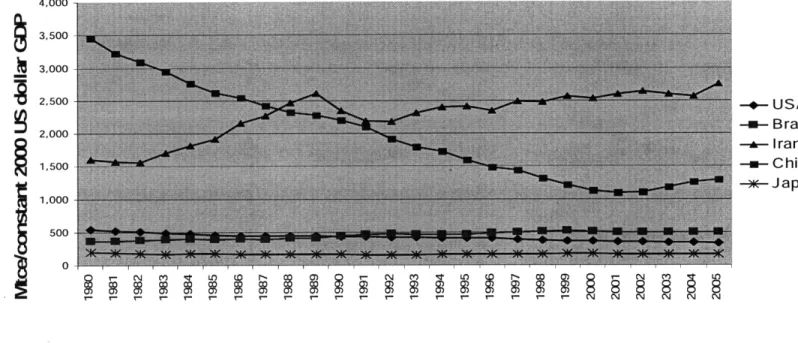
Energy intensity is defined for this study as the energy consumption per unit of gross domestic product (GDP). Polenske (2005) finds that the energy intensity of developed countries, such as the United States, has been declining steadily in the past decade, while that of the developing countries, such as Brazil and India has either fluctuated or slightly increased, as illustrated in Figure 1.

As noted below, literature reviewers identify two underlying factors that contribute to such changes: energy efficiency change and economic structural change. The service sector tends to be less energy intensive than the manufacturing and construction sectors, which are, in turn, more energy intensive than the agriculture and other primary sectors. The shifts in sectoral composition from agriculture to industry to services that accompany economic growth and development would therefore lead one to expect that energy intensity first increases and then decreases as countries grow richer (Hofman and Labar, 2007). The trend in China's energy intensity has exhibited a different pattern, however, falling by about 67% between 1978 and

2003 (Polenske, 2007). The aim of this study is to reconcile this fact with the theory.

What are the primary factors that contributed to this significant reduction of China's energy intensity? And further, what caused the national aggregate energy intensity to rebound since year

(10)

government environmental policies, state-level controls, industrial concentration, or more broadly, to the effect of China's gradual switching from a state-controlled economy to a market economy? If we can identify these factors, we can go one step further and analyze and focus on the specific roles that government policy, technology and innovation, energy prices, etc. have played and their impacts. The policy implications however will not be the focus of this study.

4,000 3,500 3,000 2,500 . USA -m-- Brazil 2,000 ra Iran 1,500oo --- China w-m- Japan 1,000 500

Figure 1: Energy Intensity of Selected Countries, 1980-2005

Notes: (1) GDP = gross domestic product, measured in 2000 US dollars using market exchange rates (2) Mtce = Million (metric) tons of coal equivalent.

(3) Units of energy consumption were converted from British thermal units to Mtce (1 Btu = .036 Mtce)

Source: Compiled by the Multiregional Planning Research Team at MIT, from Energy Information Administration (2007) data.

1.1 The Focus of this Study

My goal in this study is to contribute to our understanding of China's energy intensity change by

undertaking a statistical analysis using provincial level data. First, regional variation in terms of energy production and consumption has been pronounced especially between the inland

(11)

system from inland coal-producing regions to coastal coal-consuming regions. I find a constraint of improving energy intensity posed by the lack of transportation infrastructure investment.

Second, by adopting a similar methodology to the one used by Sue Wing (2008), I create two indexes to decompose changes in energy intensity into intra-province (efficiency) and inter-province (structural) effects. The former effect is referred to as the within index, while latter

effect is referred to as the between index. Within index captures the change of aggregate energy intensity caused by the provincial energy-intensity change, weighted by the share of provincial energy use to national energy use. This change is normally attributed to factors such as fuel prices, weather, local infrastructure investment, economic sector shift, etc. The between index captures the change of aggregate energy intensity caused by the share of provincial output change in total GDP, also weighted by the share of provincial energy use to national energy use. The major difference from previous literature (Metcalf, 2008) is that I conduct the decomposition analysis using provincial (Beijing, Jilin, Guangdong, etc) economic factors, rather than sectoral

(agriculture, industry, service, etc) economic factors.

Finally, I identify and test the various independent variables that may positively or negatively contribute to the reduction of energy intensity. In this study, I apply the decomposition analysis, instead of other methods (e.g., shift-share analysis), in order to be consistent and comparable with other research. I collect a panel dataset of 29 provinces' from 1988 to 2006 (551

observations) for analysis. I present results from the fixed-effect model regression of the energy

1 These are Beijing, Tianjin, Hebei, Shanxi, Inner Mongolia, Liaoning, Jilin, Heilongjiang, Shanghai, Jiangsu, Zhejiang, Anhui, Fujian, Jiangxi, Shandong, Henan, Hubei, Hunan, Guangdong, Guangxi, Hainan, Sichuan, Guizhou, Yunnan, Shaanxi, Gansu, Qinghai, Ningxia, and Xinjiang. Tibet, Hong Kong, and Macau are not part of this study due to data limitations.

(12)

intensity on economic- and weather-related variables, such as fuel prices, per capita income, heating degree days, etc. With provincial data, my analysis shows that the increase of per capita income and the time trend have played an important role in the decline of China's energy intensity. Heating degree days, capital-labor ratio and investment-capital ratio are positively related to energy intensity. Through an aggregation of the 29 provinces into three economic regions (north, south and west), I find that fuel price responds negatively. For per capita income, capital-labor ratio and investment-capital ratio, I include the quadratic terms in the regression to capture the non-linear effect.

1.2 Literature Review

The intensity with which countries use energy has been the subject of extensive scrutiny.

Looking first at the United States, Sue Wing (2008) decomposed changes in energy intensity into shifts in the structure of sectoral composition and adjustments in the efficiency of energy use within individual industries. He found that interindustry structural change was the principal driver of the decline at the aggregate level, while the intraindustry efficiency improvements have played a more important role in the post-1980 period. Boyd and Roop (2004) first used the Fisher Ideal Index as the basis for the decomposition of energy-intensity changes into changes in energy efficiency and economic activity. Metcalf (2008) further constructed and analyzed U.S. indexes at both national and state levels over a much longer period, between 1970 and 2003. He identified weather- and economic-related variables and used regression analysis to measure their effects on the energy-intensity change. He found that rising per capita income contributes to improvements in energy efficiency and intensity and that price changes also play a key role.

(13)

For China, Lin and Polenske (1991, 1995) applied the shift-share analysis method to decompose changes in aggregate energy intensity into structural change and efficiency change, and found that although both factors reduce energy intensity, the latter predominates. Shi (2005) also found that final demand's structural shifts, which correspond to structural shifts in energy consumption decline, did not account for as large reductions as efficiency improvements. Zhang (2003)

investigated the change in energy consumption in China's industrial sector based on a dataset for the 29 industrial subsectors. Through decomposition analysis, he found that the efficiency

change plays a key role. Fisher-Vanden et al. (2004) found that changes in industrial composition and gains in firm-level productivity both explain the continuous decline in China's energy

intensity until year 2000, while the latter is the more important driver. Lewis et al. (2003) concluded that government industrial policy was a primary factor in the energy decline, supported by ongoing programs to increase energy efficiency.

But this discussion would not be complete if it did not study concerns regarding the integrity of the data used to generate the foregoing results. Some analysts have cast doubt on China's

statistical gross domestic product (GDP) and energy-consumption data. Sinton (2001) points out that the energy data since the mid-1990s are likely to be misleading, induced by policies of the late 1990s that aimed at closing small coal mines. It is more likely that, rather than being closed, the mines disappeared from the statistics (World Bank, 2006), with the consequence of biasing calculations of aggregate energy intensity downward dramatically. As well, China's GDP data

for each year has recently been modified, with an increase varying from 0.6% in year 1980 to 16% in year 2003, based on a national poll of China's economy carried out by the National Bureau of Statistics of China.

(14)

However, all these extensive China energy-related studies are based on aggregated national data. China has over one-fifth of the world's population. One province in China is almost as large as any one of the countries in Europe. China's energy resources are unevenly dispersed, and energy intensities across the regions have significant regional variations. Although using regional data will not solve the problems with national data, it, at least, will enable us to examine more closely what is occurring with the national energy-intensity trend. Exploiting interregional heterogeneity can serve as an additional source of insights, as well as a robustness check on the results

generated with aggregated statistics. Polenske's (2006) Technology-Energy-Environment-Health (TEEH) team conducted a case study for Shanxi Province, the largest coal and coke production area in China, and they found that its energy intensity is twice that of all China. On the other hand, they also found that Liaoning Province, despite serving as the largest base for the steel-making industry, has an energy-intensity about the same level as in all of China.

There are only a few analyses using China's regional data. Auffhammer and Carson (2007), based on a provincial panel data set, exploited the considerable heterogeneity that exists across

China's provinces and clearly reject the static environmental Kuznets-curve specification. Hofman and Labar (2007) found that beyond structural change, energy intensity is negatively correlated with energy prices, the efficiency within the energy sector, and the share of light industry in provincial GDP, and positively with the share of state enterprises in industrial output. Hu and Wang (2005), by using regional data, found that the central area of China has the worst energy efficiency and its total adjustment of the energy consumption amount is over half of China's total. They also found a U-shaped relationship between each area's total-factor energy

(15)

efficiency and per capita income in that area, suggesting that energy efficiency does in fact improve with economic growth.

(16)

(17)

Chapter II

China's Aggregate and Provincial Energy Intensity

As I will show, China's aggregate energy intensity has been declining steadily since 1988 and then it started to increase after 2002, while China's provincial energy intensity has shown a much more volatile trend. I selectively identify the five most- and least-energy-intensive provinces. The provincial variance is pronounced.

2.1 Energy Intensity at the National Level

The recent rebound of China's energy intensity has raised many analysts' concerns. In order to deal with the issue of data quality, I calculate China's energy intensity by using data from three different sources. The results plotted in Figure 2 suggest that there are slight differences in terms

1988 1990 1992 1994 1996 1998 2000 2002 2004 2006

Year

Note: (1) GDP = gross domestic product, measured in year 2005 yuan; (2) tce = tons of coal equivalent. Data source: author's calculation based on data from CESYB (China Energy Statistical Yearbook), World Bank

(www.econstats.com), CSYB (China Statistical Yearbook)

Figure 2: Energy Intensity of China with Multiple Data Sources, 1988-2006

C

0

(18)

of GDP and energy consumption data. However, the GDP deflators are measured differently in the China Statistical Yearbook and by the World Bank.

Despite the small discrepancies in the absolute values, all the results clearly show a trend of energy intensity rising slightly since 2002. There are different explanations for this rebound. Hofman and Labar (2007) claim that it is, in part, ascribed to a sectoral shift towards industry in the majority of provinces, but this is offset by continued efficiency gains within industry and other sectors. Jiang and O'Neill (2005) argue that the accelerating speed of urbanization and the residential energy consumption may play an important role.

2.2 Energy Intensity at the Provincial Level

The energy intensity of China's 29 provinces shows more variety when I plot the data into one chart. The data and chart are presented in the appendix. In Figure 3, I include the five most and least energy-intensive provinces in China, ranked by the arithmetic mean of energy intensity for the period 1988 through 2006.

The five most energy-intensive provinces are Shanxi, Guizhou, Ningxia, Gansu, and Qinghai, and their total GDP accounts for only 5% of the nation's total GDP, while the five least energy-intensive provinces are Jiangsu, Zhejiang, Fujian, Guangdong and Hainan, representing 35% of GDP.

The least energy-intensive provinces are concentrated in the southern coastal area of China, starting from Jiangsu to Hainan and all of the five are border connected, forming an area that is

(19)

famous for agriculture, service, and commerce industries. The most energy-intensive provinces are landlocked, and concentrated in the inland part of China. If I include the sixth most energy-intensive province - Sichuan (including Chongqing) -, these six provinces also appear to form a continuous region. If I match the location of the identified provinces to the energy production and consumption map (Figure 4), I find a rather interesting result. The least energy-intensive regions are regions where consumption exceeds production by more than 20%. However, the

most energy-intensive regions are not those where production exceeds consumption by more than 20%, but rather production and consumption differ by less than 20%.

7.00 6.00 S5.00 - Shanxi Jiangsu 8 Zhejiang 0 4.00 -- X-- Fujian - --~Guangdo ng . 3.00 -- Hainan SS du"Guizhou i5 ~~ e "-Gansu-,-l 0 2.00 .... ... . .. * Qinghai . Ningxia 1.00 '* - National 1988 1989 1990 1991 1992 1993 1994 1995 1996 1997 1998 1999 2000 2001 2002 2003 2004 2005 2006 Year

Note: GDP is measured in 2005 Chinese Renminbi (Yuan)

Source: author's calculations based on China Statistical Yearbooks, China Energy Statistical Yearbook, and China provincial statistical yearbook (1989-2007)

(20)

SProduction exceeds consumption by more than 20% Production and consumption differ by less than 20% Consumption n exceeds production by more than 20%

,Shanghai

Tibet

(no data)

Toiwan

fainon

Sources: World Energy Outlook 2007; National Bureau of Statistics (2007); IEA

Figure 4: China's Energy Production and Consumption by Province, 2005

In the recent ten years, the most energy-intensive provinces show more volatility than the least energy-intensive provinces2_{. I suspect it is due to the fact that the extent of energy-producing} dominated inland regions, affected by national policy, and the capacity of transportation

infrastructure, can vary significantly from year to year, while the energy-consuming dominated pattern in coastal regions can be stabilized over the years.

(21)

2.3 Energy Imbalance and Regional Variance

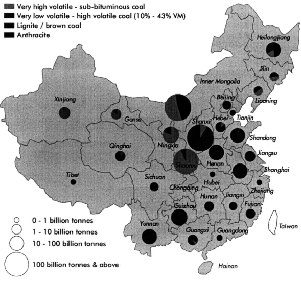
There exists a geographical imbalance in terms of China's energy production and consumption, as we can observe from Figure 5. This has raised the issues of inter-regional energy import, export, inventory, and energy transportation. While overall energy supply and demand are evening out in China, some areas continue to suffer periodic imbalances. Most of China's coal and coke is produced in a few inland provinces, such as Shanxi, Ningxia, and Inner Mongolia, while the largest centers of demand for coal and for the electricity that is generated by coal and coke, are in the coastal provinces.

M Very high volotile - sub-bituminous coal

-

Very low volatile -high volatile coal (10% -43% VM)

= Lignite / brown coal

-

Anthracite

Pn

10 - 00billion tonnes

100 billion tonnes & above , Hainon

Sources: World Energy Outlook 2007; Beijing HL consulting (2006); IEA

(22)

Inland provinces are the main energy-producing regions and are traditionally more energy intensive than energy-consuming coastal provinces. Many analysts have claimed that there is a shift from an energy-intensive economic sector towards a non-energy-intensive economic sector. With the same concept, I suspect that such energy imbalance and reverse pattern may contribute to the aggregate energy-intensity change. In other words, one possibility for why China's energy intensity has gone down over the years is that the energy-intensive inland regions have been exporting more and more energy to the less energy-intensive coastal regions. I first define coastal and inland regions, as shown in Figure 6. I then calculate the GDP, energy consumption and energy intensity for both regions, as shown in Table 1.

Coastal regions Hnan

Inland regions

Source: World Energy Outlook 2007

(23)

In Table 1, I find that the share of coastal regions' aggregate GDP has increased steadily over the years. The share of the coastal region's energy consumption is increasing, with a dip in 2001 and then decrease from 2002 to 2004. This happens to be the same period where China's national energy intensity augments. At the same time, however, the relative energy intensity has experienced first a decline, then a fluctuating period, starting from the year 2000.

Table 1: GDP, Energy Consumption, and Energy Intensity for Inland and Coastal Regions

GDP Energy Consumption Energy Intensity Year Coastal Inland Coastal Inland Coastal Inland

% of % of

% of total % of total % of total % of total Inland Inland

1988 52.7% 47.3% 44.3% 55.7% 71.5% 100% 1989 52.6% 47.4% 44.7% 55.3% 72.7% 100% 1990 52.7% 47.3% 44.5% 55.5% 72.0% 100% 1991 54.0% 46.0% 44.8% 55.2% 69.4% 100% 1992 55.2% 44.8% 45.0% 55.0% 66.3% 100% 1993 56.4% 43.6% 45.8% 54.2% 65.4% 100% 1994 57.3% 42.7% 46.5% 53.5% 64.8% 100% 1995 57.8% 42.2% 45.3% 54.7% 60.5% 100% 1996 57.8% 42.2% 45.7% 54.3% 61.6% 100% 1997 58.0% 42.0% 45.5% 54.5% 60.5% 100% 1998 58.3% 41.7% 45.8% 54.2% 60.3% 100% 1999 58.8% 41.2% 46.6% 53.4% 61.1% 100% 2000 59.2% 40.8% 48.7% 51.3% 65.5% 100% 2001 59.4% 40.6% 47.6% 52.4% 62.1% 100% 2002 59.7% 40.3% 48.8% 51.2% 64.1% 100% 2003 60.2% 39.8% 48.3% 51.7% 61.7% 100% 2004 60.5% 39.5% 48.1% 51.9% 60.5% 100% 2005 60.6% 39.4% 49.3% 50.7% 63.2% 100% 2006 60.8% 39.2% 49.3% 50.7% 62.6% 100%

Note: energy intensity for costal regions is the relative percentage to that intensity.

Source: author: China Statistical Yearbooks

of the same year inland regions' energy

I further assume that the recent rebound of energy intensity is partly due to the fact that the channel of the inland-coastal energy transportation corridor has reached its capacity due to new infrastructure investment. According to the World Energy Outlook (WEO 2007), the projections

(24)

of coal transport imply a continuing need to expand China's inland coal transport infrastructure. Shipments from inland to coastal provinces will need to increase from 507 Mtce in 2005 to 1060 Mtce in 2030 for steam coal and from 117 to 182 Mtce for coking coal.

(25)

Chapter III

China's Coal Supply, Demand, and Transportation

As one of the largest developing countries undergoing massive industrialization, China has experienced a typical increase in energy consumption to keep up with its rapid economic growth. China is already the world's second largest user of energy and the largest emitter of greenhouse gases. Official statistics show that China's energy consumption has risen from 930 million to 2,463 million metric tonnes of coal equivalent (tce) between 1988 and 2006, an average increase of 5.6% per year. During the same period, China's GDP has grown from 4,000 billion to 20,400 billion Yuan in year 2005 currency, an average annual increase of 9.5%.

3.1 Coal Production and Consumption

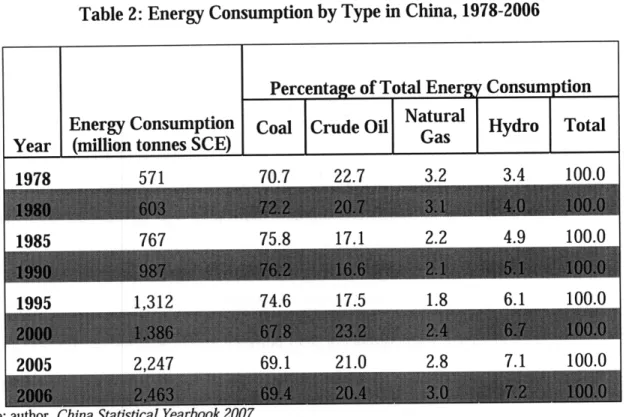
Coal is China's most important and abundant fuel, accounting for about two-thirds of its primary energy supply. China's coal output rose from 1.3 billion tonnes in 2000 to 2.2 billion tonnes in

2005, making it the largest global coal producer. In 2005, electricity generation accounted for 69% of all coal consumption in China, while cokemaking accounted for 21%. Through the study

of historical data, I find that China's dependence on coal steadily decreased since the early 1990s, while the energy provided by natural gas and hydro-power increased over the same time period

(Table 2).

Shanxi province is the largest coal- and coke-producing region in China. According to the

(26)

Table 2: Energy Consumption by Type in China, 1978-2006

Percentage of Total Energy Consumption

Energy Consumption Coal Crude Oil Natural Hydro Total

Year (million tonnes SCE) Gas

1Q72R 571 70.7 22.7 3.2 3.4 100.0

1

1985

1 2005 2,247

171 2_2 4.9 100.0

I

69.1 21.0 2.8 7.1 100.0

I

Source: author, China Statistical Yearbook

accounting for about 31% of China's total coke output versus 45% in 1998. The same year, Shanxi Province exported 5.96 million metric tonnes of coke, accounting for 47% of China's total 12.76 million tonnes of coke export.

I have not yet been able to obtain the official published data of aggregate energy production for

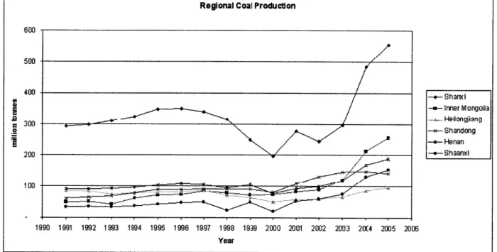
each province. However, since most of China's energy is from coal, I collected the coal production and consumption data for all the provinces from 1991 to 2005. The top coal producing provinces and consuming provinces are shown in Figures 7 and 8. I find that the highest coal-producing provinces also tend to be the highest coal-consuming provinces. In this sense, the assumption that most coal is transported from inland regions to coastal regions is not

correct. However, China's coal-fired power plants increasingly have been built around coal mines or the railway network to handle the increased amount of coal that needs to be transported

(27)

(WEO, 2007). As a result, the coal transportation issue is not a simple cross-regional raw coal-transportation issue, but rather a transmission of its secondary product--electricity.

Regional Coal Production

-- Sharxi -- Inner Mongoli3 - Heilondiang - Shandong Henan --Shaanxi 1990 1991 1992 1993 1994 1995 1996 1997 1998 1939 2000 2001 2002 2003 20C4 2005 2006 Year

Source: China Energy Statistical Yearbook 1991-1996, 1997-1999, 2005, 2006

Figure 7: Provincial Coal Production 1991-2005

Regional Coal Consumption

s Hebei -a- Shanxi --- Inner Mongolia ---- Liaoning --m-Jiangsu -e-- Shandong - Henan Year

Source: China Energy Statistical Yearbook 1991-1996, 1997-1999, 2005, 2006

Figure 8: Provincial Coal Consumption 1991-2005

4 300 200 100 300.0 250.0 200.0 150.0 100.0

(28)

3.2 Coal Transportation by Railway Systems

At present, China's coal transportation from producing regions to consumers, such as power plants, relies on rail, road, inland waterways and coastal vessels, among which railways are the

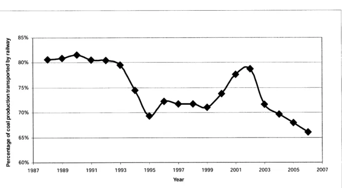
most important mode. According to the statistical yearbook, in 2006, around 66% of China's coal production was transported by means of the national railway system, as shown in Figure 9. It is also observed that although railways always remain the most important mode, the

percentage has been decreasing rapidly since 2002.

85% ... ... ... 80% 75% 0 70% 0 0 65% a, 60% 1987 1989 1991

Source: author's calculation based on

Figure 9: Percentage

1993 1995 1997 1999 2001 2003 2005

Year

data from China Statistical Yearbooks

of Coal Production Transported by National Railway

Coal transportation also accounted for about 46% of the total national railway freight

transportation in 2006, as shown in Figure 10. This percentage has been relatively constant since 1990 (43%). This raises an interesting question: as the national railway system expands, although

2007

(29)

National Railway Freight Traffic by Category of Cargo 2500 2300 2100 S 1900 0 1700 1500 -- Total . 1300 I-. 1100 900 700 --500 1988 1989 1990 1991 1992 1993 1994 1995 1996 1997 1998 1999 2000 2001 2002 2003 2004 2005 2006 Year

Source: China Statistical Yearbooks

Figure 10: National Railway Freight Traffic Coal versus Total Cargo

the volume of coal transportation increases, it cannot keep up with the increasing demand for coal that needs to be shipped from producing areas to consuming areas.

There are three possible explanations for the decreasing role of the railway mode for coal

transportation. First, there may be an increasing use of other transportation modes, such as trucks and waterways. However, this should be an involuntary result as the railway rate is around 0.12 yuan per tonne-km, while the truck rate ranges from 0.5 to 0.8 yuan per tonne-km (WEO, 2007).

Second, national railway infrastructure investment has not been able to keep up with the needs of coal transportation. As World Energy Outlook 2007 points out, much coal is transported on older trains over routes shared with passenger and the other freight trains, and there are only two

(30)

modern rail links dedicated to coal: the 600-km Daqin line and the 588-km line from Shuozhou to Huanghua. As Figure 11 shows, the average transport distance of coal, although steadily increasing, remains around 600 km/tonne in recent years. This number does not differ much from

550 km/tonne in 1990, almost 15 years ago, and it is far below that of coke and petroleum, 931

and 926 km/tonne, respectively. The lack of new investment to expand rail capacity adds constraints as coal is increasingly transported over longer distances from the deep inland production regions. However, coal-fired power plants increasingly have been built around coal

mines for the railway network to handle the increased amount of coal that needs to be transported (WEO, 2007). And once such coal-powered plant systems are established, the average transport distance of coal should not vary much.

National Railway Feight Traffic by Category of Cargo

1000 900 0 (U -- Total T .u-CoaI - Petroleum S600-( 500 400 1988 1989 1990 1991 1992 1993 1994 1995 1996 1997 1998 1999 2000 2001 2002 2003 2004 2005 2006 Year

Source: author, China Statistical Yearbooks

(31)

3.3 The Constraints of Railway Capacity and Energy Intensity

In order to test if the most important transportation mode-the national railway system-has imposed a constraint on coal transportation and further affected energy-intensity trends, I

compare the increase of the capacity of both railway freight transportation and coal production. I assume that the railway system has been fully used each year, and I used its total freight tonne-kilometers to measure the overall capacity. I used the coal production data as a measurement of its production capacity. The year-by-year percentage increase is shown in Figure 12.

20% 15% 10% 5% 0% -5% -10% -15%

Source: China Statistical Yearbooks

Figure 12: Increase of Freight Rail Capacity and Coal Production Capacity

I find that the two periods that the increased capacity of freight railway transport systems has not kept up with that of coal production are 1994-1996 and 2002 onward. When I matched the two

1989 1990 1991 1992 1993 1994 1995 1996 1 1998 999 2000 2001 2002 2003 2004 2005 2006

-.- Increase of Freight Railway Capacity

(32)

periods with China's energy-intensity chart (Figure 2), I find that 1994-1996 China's energy intensity has the smallest slope of decrease; while since 2002, the energy intensity has been increasing.

What if China's energy loop is as follows: (1) coastal regions are the main energy-consuming areas, while the inland regions are the main energy-producing areas; (2) inland regions produce and transport coal through the railway system either directly or electricity is processed locally to meet coastal regions' energy demand; (3) the coastal regions are more energy efficient than

inland regions. Such a system established from (1) through (3) can actually decrease aggregate energy intensity. The limited capacity of the railway transportation system has affected (2) above.

I believe that this has posed a negative effect and hindered the further decline of energy intensity. To analyze this issue in more depth, provincial data of energy import, export and inventory should be collected. However, at this stage, such data are not readily available.

(33)

Chapter IV

Decomposing Energy Intensity into an

Intra- and Inter-Provincial Index

Having discussed the difference of energy production and consumption patterns between inland regions and coastal regions, I now turn to the second feature of this study. It is a method used by Sue Wing (2008): an approach to decompose aggregate energy-intensity change into provincial energy-intensity change and inter-provincial structural change.

Energy intensity (ey,) can be written as a function of various components in order to capture different effects. With the decomposition results, indexes of different components can be created. Metcalf (2008) constructed an intensity index at the state level from a decomposition of the U.S. intensity index in which he disentangles changes in energy use within a sector and changes in sectoral activity over time.

4.1 Decomposition Analysis

In this study, I write the decomposition as a function of intra-provincial and inter-provincial components. The intra-provincial component captures the energy efficiency effects that are influenced by prices, technology, weather, etc, which I refer to as the "within index." The inter-provincial component captures the structural change effects, such as the increase of the share of a less-energy-intensive province's output in national GDP, which I refer to as the "between index."

Et ₁, ef, e, y,

(1) eyt - - - , Y

(34)

Where ey, is the aggregate energy intensity in year t, E, _{is aggregate energy consumption in year}

t, Y, is the national GDP in year t, ej, is the energy consumption in province i in year t, y,, is the province i's output in year t.

Salog e" a log Yit

(2)

a

log ey,

it

+ Y

at

i

_,

_t

where each weight ( w,) is the ratio of province i's share of energy consumption to the national energy consumption in year t. The left-hand side of Equation (2) is interpreted as the rate of change in aggregate energy intensity in logarithmic form. It is decomposed into two effects on the right-hand side: the change attributed to the energy-intensity change within provinces-the efficiency-change effect, and the change attributed to the change of the share of provincial output in total GDP-the structural effect.

The right-hand side of Equation (2) can be further developed into two separate indexes, I derive

Slog e" a log y"

separate equations to make an approximate calculation of the value of , t and

at

w,. wi can be calculated by using,

(3) w = ~ - x (et,. + eit_

(35)

alog

e

_alog

_Yt

And further with the Central Difference Derivative Approximation, J _{can be}

at

approximately calculated by Equations (4) and (5),

alog elt _Ae t (4) Yt Yi j, t Yt-1

at

e,

!x(

e

+ e,,)

Yit

2 yt-, y1 , t Yit c3 , Y i,t-1

alogel

A Y Y Y Y

(5)

' = -

=

at Yit 1 (Yi,t +y,,

Y 2 t Yt_,

Until this step, all the unknown components in Equation (2) have been expressed as functions of existing data variables that I have collected, namely, ey,, Et, Y, e,, y, and t. I numerically

evaluate Equations (1) through (5) using provincial GDP and energy consumption from 1988 through 2006 in Matlab and express the result as a series of index numbers.3 _{For the}

programming code, please refer to the appendix.

4.2 The Within Index and Between Index

The index result is presented in Figure 13. I find that the within index declines at a much faster rate than the between index. The improvement of energy efficiency within each province has contributed more to the change of energy intensity, than the growth of its share of provincial

(36)

China Energy Intensity Indexes 1.20 1.00 0.80 -* Intensity 0.60 i - Within_idx Btwnidx 0.40 0.20 1988 1989 1990 1991 1992 1993 1994 1995 1996 1997 1998 1999 2000 2001 2002 2003 2004 2005 2006 Year

Note: Indexes are normalized to one in 1988.

Source: author's calculation; data from China Statistical Yearbooks, and China Energy Statistical Yearbooks

Figure 13: China Energy Intensity Indexes

output in total GDP. Let me illustrate this finding by using the data in Table 1. For simplicity, there are only two regions in China, coastal regions and inland regions. In each year, coastal regions have a higher w,,, defined in Equation (3) and they also have lower regional energy intensity and a continuously increasing share of regional output. On the other hand, the inland regions have a lower w, but they have a higher regional energy intensity and a continuously decreasing share of regional output. What Figure 13 indicates is that the overall declining trend of aggregate energy intensity is more attributed to the decreasing trend of regional energy intensity (in this case in both regions), than to the fact that coastal regions produce an increasing

of total output using less energy. I also create the within and between index for inland regions

(37)

Coastal Energy Intensity Indexes 1.20 1.00 0.80 0.60 0.40 0.20 1988 1989 1990 1991 1992 1993 1994 1995 1996 1997 1998 1999 2000 2001 2002 2003 2004 2005 2006 Year

Source: author's calculation; data from China Statistical Yearbooks, and China Energy Statistical Yearbooks

Figure 14: Coastal Region Energy-Intensity Indexes

Inland Energy Intensity Indexes

1.20 1.00 0.80 eIntensity 0.60 -,-Withinidx .+--Btwnidx 0.40 0.20 1988 1989 1990 1991 1992 1993 1994 1995 1996 1997 1998 1999 2000 2001 2002 2003 2004 2005 2006 Year

Source: author's calculation; data from China Statistical Yearbooks, and China Energy Statistical Yearbooks

(38)

As we can see, both coastal and inland regions follow the same declining pattern. The coastal regions affect the overall between index more, while the inland regions affect the overall within index more.

When I compare the China energy-intensity index to the U.S. energy-intensity index (Metcalf 2008, see appendix), I find that the indexes follow the same trend. For both countries, the efficiency index outperforms the activity index. However, one thing to note is that for both efficiency and structure indexes, I am not comparing apples to apples due to the different ways of defining the "sectors" used for the decomposition analysis. In the U.S. case, Metcalf has isolated two key determinants of changes in energy intensity through separating the data by economic sectors (residential, commercial, industrial, and transportation). For him, the efficiency

change can be the price-induced energy-efficiency change within an industrial sector; while the structural change can be that the economic sector has shifted X% from energy-intensive

transportation sector into the less energy-intensive service sector. In the China case, I have separated the data by geographical units (provinces). For me, the efficiency change can be the GDP shift X% from the industrial sector to the agriculture sector within one province, thus including both efficiency and structural effects defined in Metcalf's analysis. The structural change in this study is a very different concept that is related to the share of provincial output change in total GDP. For example, Guangdong province, being very energy-efficient, thus increasing its total share of provincial output in GDP can contribute to the overall energy-intensity reduction.

(39)

Chapter V

Panel-Regression Analysis

There is considerable variation in all three indexes across time and provinces. In order to find the factors that drive changes in energy intensity, I ran regressions using provincial data between

1988 and 2006 of energy intensity (in log form) on various variables. Following the variable

identified by Metcalf (2008), I collected the data for the following factors of each province: fuel, the fuel price; pci, per capita income; pci2, the square term of per capita income; hdd, heating degree days; cdd, cooling degree days; time, time trend; time2, the square term of time trend; kl, capital labor ratio; k12, the square term of capital labor ratio; ik, investment-capital ratio; ik2, the square term of investment-capital ratio.

Table 3: List of Independent Variables

Variables Description

fuel the fuel price

pci per capita income

pci2 the square term of per capita income

hdd heating degree days

cdd cooling degree days

time time trend

time2 the square term of time trend

kl capital labor ratio

k12 the square term of capital labor ratio

ik investment-capital ratio

ik2 the square term of investment capital ratio Source: author

(40)

5.1 Dataset Variables: Expectations and Summary Statistics

The panel dataset I use contains a series of observations for each of the 29 provinces. Each province includes 19 observations (year 1988 through year 2006), with 2006 being the latest year for which data are currently (January 2009) available in the statistical yearbooks. Thus, the total number of observations is 29*19 = 551. I use a loglinear regression, aiming to find the best fit

between the data and a loglinear model.

I include the fuel price derived from the retail index of fuel from the statistical yearbooks. As the

fuel price goes up, the energy intensity (ei) should go down as residents and industry will use fuel more efficiently, e.g., drive less, improve technology, etc. On the other hand, the retail fuel prices do not reflect the price paid by some of the state-owned industrial enterprises, especially given the implied fact that the latter is largely controlled by the government. However, this price index is the only data that are readily available.

I then include the log of per capita income (pci) and its quadratic term to account for the

non-linearity effect in the response of energy intensity to personal income. As resident's income goes up, they may switch from biomass energy use to fuel energy use, which leads to a decrease of ei at the early stage. If the income goes up further, the expansion of electrical appliance use may affect ei in the other direction. The overall effect between intensity and income may appear as a

"U" shape. With the coefficients from the regression result, the value at which the combination

of the linear and quadratic terms is extreme ("turning point") can be calculated. Depending on the location of the turning point relative to the range of sample per capita income, I can

(41)

determine whether the total effect of pci is always positive or always negative or whether it changes sign at a meaningful value.

Weather can be a very important factor affecting energy use. Heating degree days (hdd) and cooling degree days (cdd) are quantitative indexes designed to reflect the demand for energy needed to heat or cool a home or business. However, I modified the calculation of hdd and cdd as follows. I multiplied a local population weight factor to reflect the weather impact on energy use. For example, one of the largest provinces--Qinghai province-has only 5 million residents (I reserve my opinion of using the term "only" here) while Beijing city alone has almost 16 million registered residents. Even if the weather pattern were same for the two provinces, the population factor should definitely be included to reflect the amount of energy use.

I include the time trend and its squared term, because as China is transitioning from an

agriculture-based economy to industrial economy, and as innovation drives technology, energy efficiency should go up dramatically. In other words, the time-trend effect can be a substitute of the effect of technology improvement on energy use.

I further include the capital-labor ratio (k/l) and its quadratic term. I deriver the capital stock from the fixed-asset investment dataset by using the perpetual inventory method (PIM). The effect of k/I ratio can go either way, for example, with a positive sign indicating increasing energy intensity with a larger share of capital-intensive heavy industries (e.g., iron and steel, petrochemicals, etc), or a negative sign indicating a transition to high-tech industries like electronics and computers.

(42)

Finally, I include the fixed-asset investment-capital ratio (i/k). The total investment in fixed assets in the whole country refers to the volume of activities in construction and purchases of fixed assets of the whole country and related fees, expressed in monetary terms during the reference period. It is a comprehensive indicator that shows the size, structure, and growth of the investment in fixed assets, providing a basis for observing the progress of construction projects and evaluating the results of investment.4 _{I discount the investment data by the price indexes of} investment in fixed assets by region (in current price). The i/k ratio is expected to respond positively to the energy intensity change. With large investments, the country is adding larger quantities of equipment, machinery, construction, and infrastructure facilities, which embody more energy-consuming ability.

For detailed data sources, assumptions, equations, and data procession, refer to the appendix. Descriptive statistics for these variables are given below.

Variable6

Ln(ei)

Ln(fuel) 1

Ln(pci)

Table 4: Summary Statistics of the Aggregate Dataset5

Std.

Description * Mean Dev. M

Energy intensity overall 0.63 0.51

-between 0.43

-within 0.27

-Retail fuel price index overall -0.84 0.58

-between 0.09

-within 0.57

-Per capita income overall 1.87 0.74

between 0.54 within 0.51 in Max 0.94 0.22 0.09 2.16 1.01 2.01 0.41 1.01 0.83 1.74 1.36 1.26 0.17 -0.69 0.34 4.03 3.23 3.00 4 Definition from China Statistical Yearbook, 2007

5 [Stata] xtsum ei fuel pci pci2 hdd cdd time time2 cl c12 ik, i(id) 6 _{Observations: N=551, n=29, T=19}

(43)

Ln(hdd) Heating degree days overall 3.79 1.29 -2.30 5.19

between 1.31 -1.64 5.07

within 0.11 3.12 4.22

Ln(cdd) Cooling degree days overall 2.92 1.43 -2.30 5.00

between 1.44 -2.23 4.73

within 0.19 1.06 3.60

Ln(kl) Capital-labor ratio overall 1.11 0.76 -0.69 3.34

between 0.59 0.13 2.60

within 0.49 -0.46 2.41

Ln(ik) Investment-capital ratio overall -1.91 0.29 -3.91 -0.64

between 0.13 -2.13 -1.61

within 0.26 -3.77 -0.93

*This table shows the min and max, std and mean in three ways that are of interest: (1) the overall sample; (2) the between sample, i.e,. x(bar)i; and (3) the within sample, i.e., xit-x(bar)i-x(global bar)

Source: author

The overall standard deviation (stdev) measures variation in the entire cross-province cross-time data set. The between standard deviation measures variation across the 29 provinces, while the within standard deviation measures variation from the province-specific data across time. For example, for the cooling degree days, the within stdev is 0.19, well below the between stdev, which is 1.44. It is because the weather does not vary much within a province from year to year but it does vary much from province to province in the same year. On the other hand, for the retail fuel price, the between stdev is well below the within stdev. It makes sense as fuel prices change much from year to year, but do not change much from province to province within the same year.

With 29 provinces and 19 years' data, I design the model as the "large N, small T" panel in which I use a large number of individuals to construct the large-sample approximations. The small T may put limits on what can be estimated. For all the variables, the within standard

(44)

deviation is non-zero, which means none of them is a time-invariant variable. There may be time-invariant characteristics that will help to explain energy intensity and its components, but these will be subsumed within the provincial fixed effects.

5.2 Fixed-Effect Regression and its Result

A panel data set has multiple observations on the same economic units. In this study, I have

collected multiple observations on energy intensity over time. In this set of panel data, each element has the characteristics of cross-regional and cross-time. As a result, panel data can have time effects, or group effects, or both.

Given the panel data, I define models that arise from the most general linear representation:

Yit = Xkitkit + it

k=1

(6) i= 1,... N

t= ,..., T

where N is the number of provinces (29), T is the number of periods (19 years), and k is the number of identified variables (e.g., pci, i/k ratio, etc). In this study, the linear representation is:

log(E/ Y) , =

a, + , log fuel, + ,2 log pci, + P3 (log pci,) 2

+ p4 log hddt, + 15 log cddt + ,6 time, + P1 time,

+ 8s log kl,t +

p9

(log kl, t)Z + ,10 lg ik,, + p,1 (log ik,) 2

The effects can be analyzed by either the fixed-effect (FE) or random-effect (RE) models. I conduct the Hausman test to decide from which model to choose. Hausman test's null

(45)

hypothesis--that the RE estimator is consistent--is rejected. The provincial-level individual effects do appear to be correlated with the regressors. I decided to start with the FE model.

Table 5: Panel Regression with FE model Fixed-effects (within) regression

Group variable (i): id

R-sq: within = 0.7990

between = 0.3146

overall = 0.3520

Number of obs Number of groups Obs per group: min

avg max F(11,511) corr(ui, Xb) = -0.8051 Prob > F = 551 29 19 = 19.0 19 = 184.62 = 0.0000

ei Coef. Std. Err. t P>Itl [95% Conf. Interval] ---fuel pci pci2 hdd cdd time time2 kl k12 ik ik2 cons 1.043143 -1.687456 .022531 .0748148 .0017877 -. 0664659 .0021448 .569478 -. 1166289 .3335833 .0704051 4.591293 .2064475 .2020048 .025861 .0536582 .0312503 .0100647 .0002643 .057302 .0223972 .1169662 .0272688 .6828185 5.05 -8.35 0.87 1.39 0.06 -6.60 8.11 9.94 -5.21 2.85 2.58 6.72 0.000 0.000 0.384 0.164 0.954 0.000 0.000 0.000 0.000 0.005 0.010 0.000 .6375529 -2.084318 -. 028276 -. 030603 -. 0596071 -. 0862392 .0016255 .4569015 -. 1606308 .1037895 .0168324 3.249816 1.448734 -1.290594 .0733381 .1802325 .0631825 -. 0466926 .002664 .6820545 -. 072627 .5633771 .1239779 5.93277 ---sigmau .66719932 sigma_e .12688754

rho .96509428 (fraction of variance due to ui)

F test that all u i=0: F(28, 511) = 54.76 Prob > F = 0.0000

Source: author

The within R-square term is 0.799, and it shows that the data are explaining a large amount of the variation in energy intensity. The estimate of rho suggests that almost all the variation in energy intensity (ei) is related to provincial differences in ei values. The F test following the regression indicates that there are significant individual (provincial level) effects. As I also observe that the corr(u_i, xb) is -0.80, standing for a high correlation between u, and the

(46)

regressors in the model, using FE model is correct. All the coefficients except for time trend represent the elasticity. For example, when per capita income increases by 1%, the energy intensity will reduce by 1.68%.

The coefficient of fuel price is positive and significant at the 1% level. It is counter intuitive as under normal market conditions, an increase in fuel prices should induce energy conservation, resulting in a lowering of energy intensity. A possible explanation is that the inventory

management behavior may play a role. Also, as discussed before, the non-market effects in some state-owned enterprises may cause energy-consumption patterns to be insensitive to the fuel price.

I observe that per capita income is negatively related to the energy intensity and is significant. Its quadratic term is positive, showing a curve opening upward. The turning point is at 37.5, which is far beyond the sample range (max=4.03). As a result, the effect of pci is always negatively related to the energy intensity change. As mentioned before, as the personal income increases, people will tend to switch from biomass to fuel energy, thus leading to a decline of energy intensity. The effect of income is consistent with the finding of Metcalf (2008) with the US data. The difference is that, with the China data, the speed of the energy-intensity change with respect to income is decreasing; while with the US data, the speed is increasing. Such a contrast

indicates that the two countries are at two different development phases. For example, switching from using coal to electricity will lead to reducing energy intensity, but not as effectively as switching from electricity to green technology, etc.

(47)

Similarly, the capital-labor ratio could go either way. Its coefficient is positive and its quadratic term is negative, and thus showing a downward curve. The turning point is at 2.43, which is well beyond the mean 1.11. The effect can be considered to be always positive to the energy- intensity change. China is a developing country and still in the middle of its industrialization process. Most of the fixed-asset investment takes place in the construction, expansion, and operation of the large utilities. When the ratio is increasing, it indicates that the accumulated fixed-asset capital is increasing, resulting in an increase of energy intensity.

The coefficients of heating degree days and cooling degree days are both positive as expected. When the heating degree days increase, the energy intensity goes up, although the t-score shows that cooling degree days have no significant impact. At the aggregate level, it makes sense because in most parts of China, heating systems, such as indoor furnaces, are available, while cooling systems (e.g., air conditioners) are not.7 _{As a result, energy consumption responds to} cold days more than to hot days.

The investment-capital ratio seems to be behaving as expected. The investment here is the total investment in fixed assets. The turning point is at -2.38, well beyond the overall mean -1.91.With increased investment, the country is adding larger quantities of equipment, machinery,

construction, and infrastructure facilities, which embody more energy consumption.

The coefficient of time trends is negative, as expected. The effect of technology improvement and innovation along time is obvious. However, the fact that the t-score is large makes me

7 _{China's rural population stood at 737 million--56 percent of the total population of more than 1.3 billion--at the end} of 2006. The ownership of air conditioners is only 7 units per 100 rural households (China Statistical Yearbook 2007).

(48)

suspect that the regression is spurious. The classical regression techniques are invalid when applied to any time-series variables that behave in a "trend-like" manner, as such techniques are only designed for variables that are stationary. However, the data I use in this study are likely to be non-stationary time series. After the first run result, I dropped the cooling degree days as it is not significant, and I dropped the time trend and its quadratic term to avoid the spurious effect.

Table 6: Panel Regression with FE model (modified)

Fixed-effects (within) regression Number of obs = 551

Group variable (i): id Number of groups = 29

R-sq: within = 0.7720 Obs per group: min = 19

between = 0.4563 avg = 19.0

overall = 0.5357 max = 19

F(8,514) = 217.49

corr(u_i, Xb) = -0.2771 Prob > F = 0.0000

ei Coef. Std. Err. t P>Itl [95% Conf. Interval]

--- +---fuel .146821 .1614133 0.91 0.363 -.1702899 .4639318 pci -1.414077 .2082578 -6.79 0.000 -1.823218 -1.004935 pci2 .1021214 .0230525 4.43 0.000 .0568327 .1474101 hdd .1070913 .0556499 1.92 0.055 -. 0022379 .2164205 kl .7482551 .0560177 13.36 0.000 .6382032 .858307 k12 -. 1422248 .0219676 -6.47 0.000 -. 1853821 -. 0990676 ik .5041655 .1221325 4.13 0.000 .2642252 .7441058 ik2 .0986575 .0287019 3.44 0.001 .04227 .155045 cons 2.600188 .6165127 4.22 0.000 1.388993 3.811383 --- +---sigma_u l .33845615 sigma_e l .13474748

rho | .8631832 (fraction of variance due to ui)

F test that all u i=0: F(28, 514) = 69.92 Prob > F = 0.0000

Source: author

As shown in Table 6, the time trend may have caused the spurious effects. Comparing the current

result to that of Table 5, I see the regression results are rather improved: the significance of fuel price has been weakened (I cast doubt on the previous result anyway); the effect of heating

(49)

degree days is significant at the 5% level; the t-scores of all the other variables are significant at the 1% level. For those variables with a quadratic term, the turning points do not vary much from previous results. The interpretation for all the variables remains the same as before.

5.3 Regression with Three Economic and Geographical Regions

China is divided into provinces, autonomous regions, and municipalities directly under the Central Government. As shown in Table 4, four out of six variables have a larger between variance than within variance. In order to capture the economic and geographical variance, and taking into account factors such as the difference between north and south, west and east, I categorize the 29 provinces into three major regions.

Table 7: China's Three Major Regions: North, South and West

Liaoning, Jilin, Heilongjiang, Beijing, Tianjin, Hebei, Shandong, Henan, North Region 1 Shanxi, Shaanxi, Inner Mogolia

Shanghai, Jiangsu, Zhejiang, Fujian, Guangdong, Guangxi, Hainan, South Region 2 Hubei, Hunan, Jiangxi, Anhui

Sichuan and Chongqing,8 Guizhou, Yunan, Gansu, Qinghai, Ningxia, West Region 3 Xinjiang

Source: http://www.china.com.cn/chinese/zhuanti/2004xdh/505635.htm

In order to avoid the spurious effect, I again drop the time-trend factor and its quadratic term. The regression result by adding regional dummy variables (code refers to appendix) is presented in Table 8.

8 Chongqing province used to be a sub-provincial city within Sichuan province until 1997. It has become the fourth municipality in China since then. In this research, I studied Chongqing and Sichuan as one combined region.

China's energy intensity and its determinants at the provincial level

By

ARCIWES

JUL 10 2009

LIBRARIES

Abstract

Acknowledgements

Table of Contents

Chapter I

Introduction

Chapter II

China's Aggregate and Provincial Energy Intensity

-

-

Pn

Chapter III

China's Coal Supply, Demand, and Transportation

1

I

I

Chapter IV

Decomposing Energy Intensity into an

Intra- and Inter-Provincial Index

a

it

at

i

,

t

t

at

at

alog

alog

Yt

at

at

at

e,

e

+ e,,)

Yit

alogel

(5)

' = -

=

Chapter V

Panel-Regression Analysis

p9

_{JUL 10 2009}

_,

_t

_t

_alog

_Yt