Collective excitations in low dimensional systems and stochastic control of population growth in a fluctuating environment

(1)

Collective Excitations in Low Dimensional Systems

and Stochastic Control of Population Growth in A

Fluctuating Environment

by

Xiang Xia

B.S., Fudan University, P. R. China (2001)

Submitted to the Department of Chemistry

in partial fulfillment of the requirements for the degree of

Doctor of Philosophy

at the

MASSACHUSETTS INSTITUTE OF TECHNOLOGY

January 2007

@

Massachusetts Institute of Technology 2007. All rights reserved.

Author

...

Department of Chemistry

/)

January 12, 2007

ert

Robert J.

Silbey

Dean of Science and Class of '42 Professor of Chemistry

Thesis Supervisor

Accepted by

...

Robert W. Field

Chairman, Department Committee on Graduate Students

OF TECHNOLOGY

MAR

3

7 This doctoral thesis has been examined by a Committee of the Department

of Chemistry as follows:

P rofessor R obert W . Field... ...

Chairman

/2

Professor Robert J. Silbey...J

...

Thesis Supervisor...

...

Thesis Supervisor

I f

(3)

Collective Excitations in Low Dimensional Systems and Stochastic

Control of Population Growth in A Fluctuating Environment

by

Xiang Xia

Submitted to the Department of Chemistry on January 12, 2007, in partial fulfillment of the

requirements for the degree of Doctor of Philosophy

Abstract

In this thesis, I study several problems in the following areas: collective excitations in con-densed matter physics, noise in gene network and stochastic control in biophysics. In the first area, I construct an effective field theory to describe Bose-Einstein Condensate (BEC) realized in an external potential. This theory explicitly explores the idea of spontaneous symmetry breaking and its application in the description of phase transitions of confined systems. Based on the effective lagrangian, I calculate the excitation spectrum and Mat-subara Green's functions using the method of functional integrals. The theory also shows that in one dimension the collective excitation of a bosonic system can be unified with that of a fermionic system, which is described by Luttinger liquid theory. The unified theory of collective excitations of low dimensional quantum systems motivates my study of collective excitations of interacting classical particles confined in one dimension. It is shown in my pa-per that the structure of Hamiltonian or Lagrangian for one dimensional constrained systems is uniquely determined by conservation laws. Therefore the excitations of bosonic, fermionic and classical particles are strikingly similar in one dimension. In the second area, i. e., noise in gene networks and phenotypic switching in a fluctuating environment, I study the noise propagation in a gene network cascade using the method of master equations which examines the validity of the more popular methods such as the Langevin equation. To further explore the applications of stochastic processes for complex systems, I study phenotypic switches in a fluctuating environment. By combining the techniques of stochastic differential equation and stochastic dynamical programming, I propose a simple framework which can be used to study phenotypic growth dynamics. Another work is to explore the influence of environment on the dynamical properties of small systems is directed to the unusual blinking statistics of semiconductor quantum dots. I show in a model system that a broad spectrum of decay rates is possible when disorder is present in the environment.

(4)

(5)

Acknowledgments

At the time I am about to finish this Ph.D. thesis, I find the most difficult part is the Ac-knowledgements. A physical picture can be drawn nicely in several equations; the equations can be displayed beautifully using the magic of Latex; however, it is far beyond the abilities of any of these to express my gratitude to so many people. In this sense, my acknowledgements are incomplete. The guidance that I have received, the friendship that I have developed and so many memorable moments will persist. Never forget.

First and foremost, I am grateful to my advisor Professor Robert J. Silbey. Bob is a keen scientist and at the same time he is a very good listener. He can always understand my idea. in the shortest time, ask deep questions and provide immediate guidance. Moreover, Bob has always given me freedom to pursue any of my research interests, which turns out to be very rewarding since it helps me to develop my scientific taste and philosophy. Beside academic guidance, Bob is always ready to provide suggestions on diverse topics from jazz to national parks. Without him, I wouldn't have grown into a true scientist.

I am also grateful to Professor Jianshu Cao. Professor Cao has consistently helped me to sharpen my physical idea of several problems. He also suggested that I learn many valuable mathematical techniques, which are indispensable to my research.

I particularly thank Professor Robert W. Field and Professor Keith A. Nelson for their careful reading of the manuscript. Professor Robert W. Field has always been kind to new and old Ph.D. students, helping us with our courses and research, while Professor Keith A. Nelson helped me to know more about MIT through emails, after I had received the offer letter from MIT. I also would like to thank Professor Moungi G. Bawendi for his support to my thesis proposal.

Throughout my study and research at MIT, the everyday's life in the 'zoo' is always enjoyable. This could not have been possible without the friendship with former and cur-rent members. I have benefitted a lot from numerous discussions with Serhan Altunata, Jim Witkoskie, Jaeyoung Sung, Yuan-Chung Cheng, Jianlan Wu, Shilong Yang, Vassiliy Lubchenko, Steve Presse, Ophire Flomenbom, Tobias Ambjornsson and Qin Wu.

(6)

My special thanks goes to mny parents Tialnguan Xia a~nd Hui Cai for their love, support and their trust in me. La.st, but not the least, I am. particularly grateful to Jing Xu for her love, understanding, encouragement, support and trust in me. Without you this thesis would not have been possible. My Ph.D. thesis, therefore, is devoted to them.

(7)

5 Dynamic Phenotypic Switching: Influence of a Fluctuating on Population Growth 5.1 Introduction . . . . ... 5.2 2-phenotype model . . . ... 5.3 Optimal Allocation and the Selection between Responsive and notypic Switchings . . . ... 5.3.1 Power Fitness Function ... 5.3.2 Logarithmic Fitness Function ... 5.4 Lyapunov Exponent . . ... Environment 129 . . . . . . 130 131 Passive Phe-... 133 . .. 135 . . . 139 . . . 141 Sensing Delay ...

M-phenotype and Phenotypic Redundancy . . . . . . . . . ..

Conclusions ...

Appendix A: It6 Calculus, Martingales and Diffusion Properties . . . . 142 146 149 151

(9)

5.8.1 Standard Brownian Motion Z ... 151

5.8.2 Ito Integral and Itf's Lemma . ... ... .... 152

5.8.3 Martingales ... ... .. 154

5.8.4 Diffusion Properties ... ... .. 155

5.8.5 Jensen's Inequality ... ... . 156

5.9 Appendix B: Dynamic Programming and the HJB Equation . .... .... 156

(10)

(11)

List of Figures

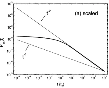
3-1 Probability distribution functions for the on time in the delocalized regime. Universal on-time probability distribution function obtained by scaling in a.

characteristic on-state lifetime to = 1/F 0. . . . 78

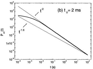
3-2 Probability distribution functions for the on time in the delocalized regime. Po,,(t) for a QD/SM with a lifetime 2ms and a fixed observation window. The exponents of the fitting power laws lie between -1.6 and -2. . ... 79

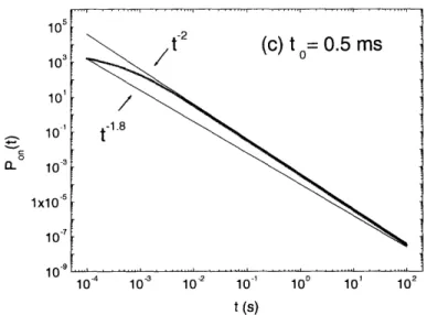
3-3 Probability distribution functions for the on time in the delocalized regime. Po,, (t) of a QD/SM with a shorter lifetime 0.5ms. The exponents of the fitting power laws lie between -1.8 and -2. ... ... . . 80

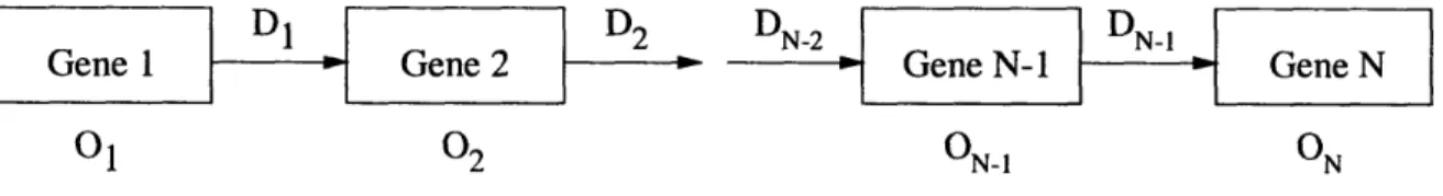
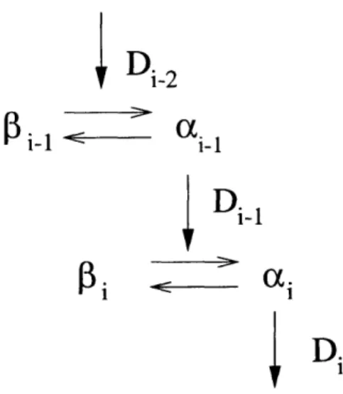
4-1 One Dimensional Chain Model ... ... 93

4-2 Regulation and Gene Cascade ... ... 94

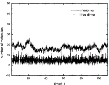
4-3 Time Trajectories of Protein Numbers by Simulation ... ... 114

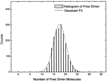
4-4 Protein Dimer Number Distribution and Gaussian Fit. The histogram is obtained from computer simulation and a gaussian distribution fits well to the histogram. ... ... .. 115

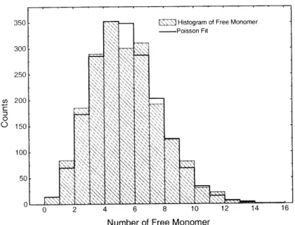
4-5 Protein Monomer Number Distribution and Poisson Fit. The histogram is obtained from computer simulation. A gaussian distribution cannot fit the histogram. A good fit can be obtained by a Poisson distribution. ... 116

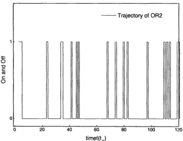
4-6 The trajectory of the active operator state OR2 shows an on and off dynamics. See appendix for detailed description. ... ... 117

(12)

4-7 Dependency Graph: Each chemnical reaction is denoted a.s a node and the influence of one node i to another node j is indica~ted as an arrow pointing

(13)

List of Tables

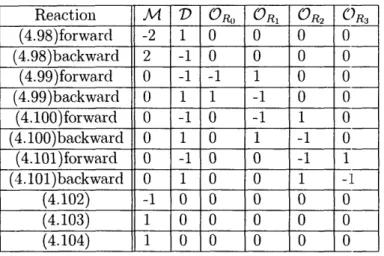
4. 1 State Vector Change Table: The state of the system at any point in time is characterized by a, state vector S. Its elements change when chemical reactions occur. ... ... ... 119

(14)

(15)

Chapter 1 Effective Quantum Field Theory for

Bose Einstein Condensate

Ordinary phase transitions occur at a true macroscopic level; however, quantum phase tran-sitions are are much more difficult at this level. Experimental realization of these types of phase transitions are usually achieved in extreme conditions: high magnetic/electric field, extremely low temperature and state of art nano-fabrication, which are all aimed at achieving geometric confinement. From the theoretical point of view, a confined geometry is necessary since the mean energy spacing is inversely proportional to the size of the system. Therefore one of the solutions to reduce thermal effects is to set up an artificial confining potential. This also brings challenges to theorists as most of the standard phase transition theories and quantum many-body theories assume an infinitely large system and no spacial confinement. Even though certain symmetries are not available at the onset, new constraints, nevertheless, show up. In addition, the nature of phase transitions is not changed by confining potentials because it only relies on those symmetries that are spontaneously broken. These in fact are some of the keys that lead to successful theories. In this chapter we focus on one type of con-fined phase transitions, namely, Bose-Einstein Condensation (BEC) realized experimentally since 1995. We adopt an effective-field-theory view to describe the low-energy excitations of trapped Bose gases, which allows a direct and systematic way to investigate the

(16)

conse-quences of spontaneous synunmmetry breaking. The derivation of the effective La.grangian can incorporate various approximations and can reproduce the results obtained by the standard hydrodynamic approach. Based on the effective Lagra.ngian, we calculate the energy spec-trum and Ma.tsubara. Green's function of trapped 1D Bose gases with (-function repulsive interaction, allowing the comparison of various results obtained by different approaches. We also analytically calculate the finite-temperature correlation function of trapped 2D Bose gases. The calculation scheme can be easily extended to higher dimensions. We find that particle interactions will always decrease the coherence length of the condensate in 2D, con-firming recent numerical results. The validation of various asymptotic expressions are given.

1.1 Introduction

The problem of theoretically describing interacting Bose gases at low temperatures has a long history. Unlike fermionic problems, where by particle-hole transformation Wick's the-orem can be applied, conventional perturbation theory can not be applied to bosons since neither creation nor annihilation operators annihilate the ground state, and a.s a result the application of Wick's theorem becomes much more complicated. The successful perturbative approach of Bogoliubov [1] is based on the observation of vanishing commutator in the ther-modynamical limit (N -

oc,

V -- oc, N/V --+ constant) and separating the creation and

annihilation operators of the ground state into a c-number part and an operator correction part, which is assumed to be small. Bogoliubov's perturbation theory provides the basis for the modern theoretical treatment of the Bose-Einstein condensation(BEC) in a confining external potential, which was experimentally realized in 1995 [2].

The standard starting point of the modern treatment for nonuniform Bose gases at low temperatures is the Gross-Pitaevskii (GP) equation [3]:

ihOtT(r, t) (= V2

+

Vext(r) + gl(r, t)12) (r,) (1.1) 2meter _{or wave} function of the _condensate, V(r) is the where T(r,t) is the order parameter or wave function of the condensate, Vext(r) is the

(17)

confining potential and the coupling constant g is related to the s-wave scattering length a

by:

rg

_(1.2)

The GP equation can be interpreted as a self-consistent Hartree equation for the

conden-sate wave function, so it does not include the effect of the interaction with noncondenconden-sate

atoms. In order to study low energy collective excitations, Stringa.ri[4] developed a

hydro-dynamic approach, in which the GP equation is linearized in terms of density and phase

fields. Tile collective excitations are sound waves with a modified dispersion law caused by

the confining potentials. The hydrodynamic approach was further developed by Griffin et

al. [5] where the classical density and phase fields are quantized and the sound waves become

phonons. The hydrodynamic approach was applied extensively to study the excitation

spec-trum and phase coherence of Bose gases in deformed traps at T _ 0 [6, 7, 8]. It was found

that confining potentials play such an important role in suppressing quantum and thermal

fluctuations that dispersion laws become discrete and there exists non-exponential decay

of off-diagonal long range order, which indicates possible BEC at finite T in 2D and ID.

Numerical study [9, 10, 11] of collective excitations of BEC at finite temperatures were

im-plemented by the finite-temperature Hartree-Fock-Bogoliubov(HFB) method. It was shown

that the excitation frequencies have a weak temperature dependence while the condensate

fraction is strongly depleted. Numerical calculations indicate disagreement of theoretical and

experimental results at finite temperatures, so it would be desirable to obtain the Matsubara

Green's functions for trapped gases analytically and give explicitly the validity conditions

for various asymptotic expressions.

The hydrodynamic approach based on the GP equation, although powerful and efficient,

may not be the most natural method for discussing the finite temperature behavior of

inter-acting Bose gases. It is known that field-theoretical quantities such as the Green's function

and vertex function can be expressed directly as functional averages. Furthermore, it is an

advantage to study low energy physics in effective field theories facilitated by the functional

method, see eg. Ref.[11] for a recent review. The functional approach to superfluids was

(18)

developed by Popov [13], where the infrared-singularity difficulty encountered in conven-tional perturbation technique was alleviated by the miethod of successive integration over fast modes. One essentially obtained anll effective field theory in terms of renormalized cou-pling constants and slow modes. This approach was further developed by Bogoliubov et al.

[14, 15, 16] to study BEC in confined potentials. A slightly different way to obtain the ef-fective Lagrangian was adopted in [17, 18, 19], where a. polar coordinate transformation was performed first. In this paper, we view BEC as a result of spontaneous breaking of global

U(1) symmetry and derive an effective Lagrangian of the corresponding Na.mbu-Goldstone bosons for the general cases of trapped Bose gases. Despite the recent developments of techniques for calcula.ting correlation functions in BEC, the confining potential makes the

problem quite complicated so that one must resort to approximations and regulations in

order to obtain simple asymptotic behavior, which leads to different results, e.g. for conden-sate density [7, 16], exponents of the 1D equal-time single particle correlation function power

law etc. So it is importanlt to compare alnd unify the results obtained by hydrodynamnic and functional approaches.

1.2 Effective Lagrangian Approach

1.2.1 Derivation of Effective Lagrangian

Let us consider a weakly interacting Bose gas confined in an external potential Vext(r) in

D + 1 dimensions. The partition function can be written as:

Z[

*, ]

=

*D

e-

fdf

dDr

(1.3)

where the Euclidean Lagrangian £ is

£

• * + •, V*V + [Vext(r) -_ •* +

9D

(*)V 2 (1.4)

(19)

The bosons interact with 5-function repulsion and 9D is the coupling constant. Here /3 = '

and p. is chlemical potential. It is clear that the Euler-Lagrange equation of motion for the field VY* yields the GP equation (1.1) with T -- it/h. To facilitate the analysis of spontaneous

symmetry breaking, it is useful to absorb the third term in (1.4) into the interaction term to obtain:

£

=

*a,

+

**VI*VO**

+ V(VV,)*

(1.5)

2mn and V((*) = (*, - po(r))2

_(1.6)

2

is a field potential, of which po(r) is the potential minimum:

p0(r)

= [M

-

Vext(r)] (1.7)

9D

It is clear £ is invariant under a global U(1) symmetry transformation:

'

--ei (1.8)

The Goldstone theorem predicts the existence of massless bosons when the global U(1) symmetry is spontaneously broken. Since we wish to construct an effective Lagrangian for low-energy processes, the Nambu-Goldstone boson field must a.ppear in the effective Lagrangian. It is well-known that the Nambu-Goldstone boson is completely decoupled in the limit of vanishing momentum. This implies that, by a proper transformation of field variables, the Nambu-Goldstone bosonic field should drop out of field potential term,

V(V*

4)),

and this naturally suggests the following choice for field variables:

C(r, 7-) = (r, T)ei(r) (1.9a)

(20)

Under the transformation (1.8), 0 transforms a.s: 0 -> 0+a, where (v is a constant. Since C is

invariant under this transformation, the effective lagra.ngian £ef must contain 0 in derivative forms to preserve the symmetry. A general form of L£ff can then be written as:

Lef.

=

I

ojji0,00,,0 +

h.d.t.

(1.10)

where g,,,, can be interpreted as an Euclidean metric tensor. For an inhomogeneous situation

g,,, can be different from a constant metric. h.d.t. denotes terms in higher powers of a,,0 and coupling terms of a,,0 with other degrees of freedom. In the low energy regime, by power counting, only the first or the first few terms in (1.10) are needed. Working with the effective Lagrangian, Leff, should allow easier calculations and give same results as those obtained by original Lagrangian C.

Now we will perform the matching process as the following: By appropriate scaling, i.e. 6 ---+ _.-_5', one finds £ -- - _.-_9D So gD plays the role of h, when gD is small, and we can use

the semiclassical approximation, namely setting all derivatives to zero and minimizing the field potential energy, to obtain the Thomas-Fermi ground state configuration:

PTF(r) = po(r)0(po(r))

I- [ - Vext(r)]'d (i - Vext(r)) _(1.11) f]D

where iV(x) is the step function. The ground state configuration (1.11) is valid provided that physical bosons are weakly interacting. The condensate density, PTF(r), can also be obtained from the GP equation using the TFA. By choosing this nonzero ground state configuration the global U(1) symmetry is spontaneously broken. Define the dynamic density:

p(r,•) - #*(r,7) (r, )

pTF(r) + a(r, 7) (1.12)

(21)

fluctu-ating density a(r, r) generally includes contributions from thermal and quantum fluctuations of the condensate and the non-condensate. At low temperatures, we expect

PIT(r) > or(r, T) (1.13)

In terms of p(r, 7) and 0(r, T), the Lagrangian becomes:

1 + p 5-1 - (p)2+p + V1

= -9,p

+

ip 0 (Vp)2 2 + D(P - po)2 (1.14)

2 2m 4p 2

The first term is a. total derivative and can be dropped. In the low energy regime, (1.13) holds and we can expand (1.14) in powers of - using (1.12):

h2_T

V

L = ipTFO + -PTF )2

S2m 1

V

In

- Va -

4

(V lnpTF)2a

i(

2 - gPa9 (-po) + i(0O)U

[1

2h

_h

_(V

-D

g+

t2

lnn+

2 -- a In PTF- VaI(Va)

2 8mpTF 8mpTF 4mpTF

+0 ((P0F) 3) (1.15)

The first, line describes the dynamics of the phase field 0(r, 7). The second and third lines are coupling of fluctuating density field a(r, T) with the static condensate and the phase field (phonon excitations) in linear and quadratic orders of - . For low-energy processes, it is

sufficient to truncate the series at the quadratic level and the contribution from a field can be easily evaluated. On the other hand, if one is interested in noncondensate dynamics, the 0(r, T) field should be integrated out instead for the effective Lagrangian. Now by integrating over the a field, we arrive at:

(22)

C=

i00 + (VO)2 -

2 (2V

2

I

TF

+ (V

l

n

TF)2 1 x 2 K [V2 + 2V In PT. - V - (V In PT )2] - 2gD

Si8o +

(VO)2

-_7h

(2V

2

l PT

F

+

PT)2)

+

TF

)2

21n

8

27

(1.16)

where we dropped the term iPTFT-O, which essentially imposes the conservation of PTF.

The following scaling analysis will help to simplify (1.16): V2_{, 2V In}

PTF -V and (V In PTF)2

scale as R- 2 and they should become negligible to 29g at large distances. We can define a length scale ( such that:

It2 2 2mpTF -2 = 2g9 2 MnPTF ý2 i.e. h(r) = _(1.17) V/2mpTF(r)gD

above which we can safely neglect the gradient terms in the demonimator of (1.16). We see that ((r) defined above is just the healing length and it is a spatially dependent quantity due to the confining potentials. ý(r) is larger near the edge than in the center of a trap. The approximation we made here is often called TFA, originally proposed to calculate the electron density and potential energy of atoms self-consistently[20]. It is useful to estimate the ratio of healing length ý to the average inter-particle distance d in 3D: d = ()1/3.

Given the coupling constant g3 in (1.2), (3pa)p -1/6. Typical values of Bose gas density

in experiments range from 1013 _ 1015cm- 3, while the scattering length a

-

10-7cm, so

O(1). In studying long wave length collective excitations, the above simplification is well justified. In addition, from dimensional analysis and matching (1.16) to (1.10), we only need to retain derivative terms up quadratic order. So we finally arrive at the following

(23)

effective Lagrangian:

Leff = 2K(r) v

(a

0 ₎2 _{+ hv(r)(VO)2]} _(1.18)

where

v(r) = gDTF(r) (1.19)

can be interpreted as the local velocity of sound. The interaction parameter K(r):

K(r)

=

(1.20)

h

PTF(r)

is inhomoge-neous due to the confining external potential. It is straightforward to show that the Riemann tensor is non-vanishing, so the effective Lagrangian (1.18) describes a massless scalar phase field 0(r, 7) in a. curved spacetime. We see the Nambu-Goldstone boson field indeed results from the nonvanishing of order parameter in ground state, which spontaneously breaks the global U(1) symmetry. In 1D and with vanishing external confining potential, the effective Lagrangian(1.18) also describes the Luttinger liquid of interacting fermions. An operator approach to the 1D quantum liquid was given by Haldane [1].

1.2.2 Matsubara Green's Function

To discuss finite temperature correlation and linear response, it is desirable to calculate the Matsubara Green's function defined by

(24)

where T, denotes ina.ginary-tinie ordering. In the functional representation the Matsubara Green's function can written as:

(r, -; r', T')

. "

J D O *D· e- f( J l' d" l,·.r.,X,

.1

f

EDpDO

p7(r,

T)p(r',

T)

ei(r,')-O(r',T')]-

,dT f rl•Dl[p,O]

f

DpDO

e- I(l)" dr J (dIlr[p,o]

(r)pT (r) Oei[O(rr ) - (r',r')]-f ' -r f f IDr ff(O1

- pyTF(r)pTF (r') 0 (ITf d DrCf[O

f DOe-- fo dT f dDrIef[0]

= V/P-TF(r)PTV(r')(Tei [O(r,r)-O(r',r')])

In the second line, we use the fact that the density fluctuation is small (1.13) and therefore can be neglected. Since the effective Lagrangiain (1.18) is quadratic in 0(r,7), 0(r, T) is a linear function of bosonic operators. For any function of linear bosonic operators we have the identity:

.2 -2

(eflef2) e e(hfl2+;(l + f2)) (1.22)

So the Matsubara Green's function becomes:

g(r,

r;

r',

T')=

-v/ pT• (r)pTF(r') e

'e'

(1.23)

and

F(r,

7; r', T')

9 (0) (r, r; r', T') -

[g(O)(r,

7; r, 7) + G(0

)

(r',

T';

r', T')] (1.24) We thus reduce the '• field Matsubara Green's function to the calculation of the 0 field Matsubara Green's function 9(0)(r, 7; r', T'):

(25)

which satisfies:

S+

-V

-(pTF(r)V) g(0)(r, T; r', T') (r -r')(T - 7') (1.26)

For vanishing external confining potential, by appropriate scaling, (1.26) is just the Green's function fo:r D+1 dimensional Poisson equation with periodic boundary condition in the

'ý direction. For the inhomogeneous case, PTF(r)

$

constant, one should be careful when

specifying the boundary condition for G(0)(r, 7; r', T') [6]. Since we are working at length

scales no shorter than the healing length (1.17), there is ambiguity in the regions where

pTF(r) = 0. It is natural to impose the natural boundary condition:

1G() (r, 7; r', /') I < 00 (1.27)

from the fact that V) and its normal derivatives are bounded.

1.3 Matusbara Green's Function for Bose Gases in

Har-monic Traps

1.3.1 ID Trapped Bose Gases

The correlation function for an unconfined 1D quantum fluid has been discussed extensively in the literature [1, 1, 24]. The problem of homogeneous interacting bosons can be related to the problem of interacting fermions by Jordan-Wigner transformation [22] and they both can be described by the same effective Lagrangian (1.18), except for possible redefinition of parameters. We simply have to solve:

(26)

which, with (1.24) inserted into (1.23), yields

(1.29)

g(r,

-; r'.') =

sinh [j•[r - '1 + Ihv(T - T') + d]1

[31 .,

with gas density p , velocity of sound 91V

V =P

(1.30)

and interaction parameter

h P= (1.31)

d is a. short distance cutoff parameter, which regularizes the theory. The scaling exponent:

27 27rhp

SK nmy (1.32)

ha.s pure quantum nature even at finite temperatures. The one-body density matrix n(r, r') = -g(r, 7; r', T + 0+) (1.33)

which characterizes long-range order, decays exponentially at finite temperature:

n(r, r') c e (T) (1.34)

where the coherence length is found to be

A(T) = 2h2

rnkBT (1.35)

Obviously, there is no quantum degeneracy when A(T) < -, which sets an upper bound for

(1.29) to hold:

h

2_p2

(27)

At T -+ 0, however, there exists quasi long-range order since n(r, r') decays as a power law. The zero teml)erature Green's function is given by:

G(r.

t;

r',

t')=

(r

,(,.,

t)

tb(r',

t'))

=

p

(1.37)

S[7. -7'

-

v(t

-

t')

+

d](

which shows the feature of Lorentz invariance of the effective La.grangian. The speed of light is replaced by the velocity of sound and the correlation function decays as a power law.

Now let us consider a harmonic external confining potential:

Vext(r) = -rnw227 (1.38)

Since the effective Lagrangian approach is only valid under the condition (1.13), it is neces-sary to find the classical turning point(surface) Re set by

Vext(Rc)

=

(1.39)

Physically R/ determines the size of the condensate within TFA. For ID and the harmonic potential (1.38):

Re

=

(1.40)

mz

Define dimensionless parameters:

X-=

_(1.41a)

Re a = _(1.41b) then PTF(r) =- (1 - 2_)•9(1 - xi) (1.42)

Perform a mode expansion:

g()

(r, T; r', T') = - e-iw r(r-r')()

(r,

r',

w,)

(1.43)

(28)

where 0,, = is the Matsubara frequency for bosons, and substitute (1.42) (1.43) to (1.26), we get: [(1 - x2)O- - 2.x,: - n.2d] q(, ::', n) = 6(x - x'),

_{Ix <}

1I

(1.44) where 2- Ln

g(x,:, x,', , =

291

c

(0) rh".

, , )

The homogeneous equation to (1.44) is the Legendre equation. (1.27) requires the following eigenfunction expansion:

O0

S(:,

:', na) = •

,,,

(X',

na)P

(x)

71=0

where P,(:r) is the nth Legendre polynomial. Notice that

(1.45) The boundary condition

(1.46) 7n=O We obtain: 00 1 g(x,

x',

na =

0)

=

-

m(m 2 2

Pm(X)

m=O( +1) + 2a g(x,x', a (1.47a) (1.47b) oo 1

0)

2 m+

2 Pm(x)Pm(x') S M m(m + 1)

The n = 0 mode (1.47b) corresponds to static correlation. Substituting (1.47b) into (1.43) and performing the sum exactly[25], we obtain the static phase field Matsubara Green's function:

g0)

(r, r') S1 (0)(r _,r' W, _{= 0)} -- OP -1 I In

6(T)

jr -₊_2R-r'l2) 2Rc (1.48)

+

,)Pm

(,Z)

Pm(X/)

1[

(29)

which contributes to the static part of (1.24):

F (r

r') =

26(T)

i

(1

,)(1

<

)

(1.49)

where 2h2pTF(0) A(T)

=(T)

- (1.50) mnkBTR, R.

A(T) is the coherence length defined in (1.35). Due to finite size of the sample, it is possible

to define a characteristic temperature To [26] such that A(TO) = Rc, i.e.

2h2pTF(O)

TO = (1.51)

rmkBRC

At T < To, the coherence length exceeds the sample size Rc, and both density and phase fluctuations are suppressed. A true condensate can be realized. Notice that F,(r, r') in (1.49) agrees exactly with that obtained by the hydrodynamic approach [8]. A similar expression was given by Bogoliubov et al. [16] using the functional method; however, their results have a different expression for the velocity of sound.

The dynamic part (1.47a) can also be summed exactly to give:

)(r r')= h2w2R sin(v,,r) ,, (1.52)

where

1 1

nv, = -

₂

+ f -

₄

- n2a2 (1.53) and r> - max{r, r'}, r< - min{r, r'}. Pvn (x) is the Legendre function of the first kind. It

is well known that by analytic continuation, iw, -- E + i6, the Matsubara Green's function becomes the retarded Green's function, whose poles give energy spectrum. From (1.52), we see that these poles are located at vn = m, m = 0, 1, 2, 7 • -. So the energy spectrum is

m(m + 1)

(30)

This result agrees with [16] but different from that of [4, 6] for quasi-1D trapped gas:

E,m

=-

,

•-

m(nI

+ 3)

(1.55)

2

The difference is due to the average over radial degrees of freedom of the latter work.

For temperatures:

T> h

2 v rkB

we have Ivj > 1 and we are justified to use the following expansion [19]:

P, (cos ý) = - cos +

v sm

'in

(1.56) (1.57)

4-4

with 0 < E <

cp

< 7 - E; v > 1, or equivalently, r, r' << R,. In fact, this expansion can be

applied to much lower temperatures and r, r' - R, for the following reasons:(1)Large juvI

can also be ensured by large n in (1.53), so the expansion (1.57) works better for higher modes;(2)The TFA breaks down near the trap edge, so errors in extending r, r' to R, would be within that of TFA. To order _,

₍

_wefinwe find

(1.58)

() (r, r', Wn)=

cosh

no

7

-dh2Waa (r, r') RI n _I _RC where a(r, r') TF()+ PTF(') 2 4PTF (O)

Substitution of (1.58) to (1.43) leads to a dynamic correlation function:

9() (r, T;r 7 , T') 1 y(r, r') 1

+

(r, r')

/3hv(O)

sinh

___

1 In v

sinh v(

[Ir - r'l + ihv(O)(r - -r') + d]

prd hf3hv(O) I

In

sinh

[

[2rrR, -

Ir

- r'l + ihv(O)(w - T')] I

rd

L3hv

(0) 1) (1.60) (1.59)

12

21 c

+O

(31)

with a, spatially-dependent coefficient

(,

27rrhpTF(O)(r, r')

m(y( 0))= (1.61)

It is clear that in the limit R, -> oo, -(r, r') reduces to the result of untrapped gas (1.32).

The phase field Green's function

•() (r, 7; 7-', 7') = 90) (r, r') + (0O) (r, 7; r', 7') (1.62)

together with (1.23) and (1.24), yields the following Matsubara Green's function for 1D

trapped bosons in a. harmonic potential:

g(

7;

r-T')

-r,

-

T)

v•()

sinh

[--() - r'l /r + ihv(0)( _- _T')

_{+ d]}

1 x1 [sinh [([27rRc-

-r-

r' + ihv(O)(r - 7')]] r' (1.63) where (r, r', T) = PTF(r)PTF(r')exp (T)In R(1 )(1 (1.64)

is the renormalized static density correlation function, which comes directly from the static contribution of the phase field F,(r, r'). Note the following features of trapped 1D boson gases: (a) At finite temperatures, the off-diagonal long range order n(r, r') is determined by static density correlations, while for untrapped gases it is the dynamic correlation that contributes. Indeed, expanding ((r, r', T) to lowest order in -I- and • gives

jr-r'11

n(r, r') - e- A•T) (1.65)

(32)

decays faster than this exponential behavior a.s seen from the logarithm in (1.64). Physically this can be understood because in the vicinity of trap edge, the healing length is much larger than in the trap center, so the actual condensate size is smaller than R,; (b) At T = 0, only

the dynamic Fi(r, T. 7r', T') contributes to

g(r,

7; r', T'). The inhomogeneity shows up

as

spatial-dependent exponent (1.61), which involves an average over the condensate density a.t r and r'. This spatial-dependence, which is absent in untrapped gases, is a higher order

effect and it is difficult to detect if the analysis is restricted to the region of trap center. In fact, as Rc -- oc, F,(r, r') vanishes, and the second term in g(O )(r, r; r', T') (1.60) becomes a.

constant and does not contribute to Fd(r, 7; r', T'). So g('r, T; r', T')

(1.63)

would only include the first term thereby reducing to the Ma~tsubara. Green's function of untrapped 1D Bose gases (1.29), as it should.

It is useful to compare our results for 1D trapped Bose gases with that obtained by the hydrodynamic approach, for exaimple,[8, 26] and the functional approach of successive integration of fast modes (SIFM) recently adopted by Bogoliubov et al.[16]. We find that (a) our results agree exactly with hydrodynamic approach for the static correlation function and condensate parameters such as condensate density and velocity of sound, but are differ-ent from that obtained from SIFM; (b) in the quasi-homogeneous limit, our results for the dynamic correlation reduce to the same functional form as that obtained by SIFM. How-ever, our spatial-dependent exponent -y(r, r') (1.61) depends on an inhomogeneity expansion

parameter

PTF(r) + pTF(r')

(1.66)

4_PTF(0)

whereas in SIFM the exponent depends on condensate density at F(---) only. Unfortu-nately, analytic results from hydrodynamic approach are not available for comparison so far; (c) we find that static and dynamic correlation play different roles in the off-diagonal long range order for trapped 1D Bose gases at different temperatures, while SIFM suggests that only dynamic correlation contributes. In principle, within the TFA, all approaches should give the same results for physical quantities. We think the discrepancies arise mainly from technical aspects: In SIFM, one must first integrate over fast modes exactly to obtain an

(33)

effective Lagrangian. This is practically not possible due to the new vertices generated by interaction [13]. So any particular approximation made in this early stage would inevitably

introduce uncertainty in the renormalized coupling para-meters like condensate density,

veloc-ity of sound and so on, which bring about the differences in the final results. A second factor that accounts for the discrepancies comes from boundary conditions. We find it physically appealing to use the natural boundary condition (1.27).

1.3.2 2D Trapped Bose Gases

Now let us consider a 2D Bose gas confined in a harmonic potential:

Vext(r) = -mw21 r2 (1.67)

2

where w1 is the radial trapping frequency. The classical turning surface is found to be:

Rc = (1.68)

The condensate density is:

pTF(r) = (1 x2)0(1 -) (1.69)

g2

where x = ~. In cylindrical polar coordinates

V = 1rer + 1-0~¢ (1.70a)

1 1

V2 =

r(rr)r

+

1 (1.70b)

6(r- r') = -6(r - r')6(¢ - 0') (1.70c)

(34)

(1.26) becomes: 1 0

-

+ -'2Pr (r)

1

,r + + -rpTFy(r)O,. 9(0)(r,

T;

T71

-0(T

-

T

)6(r

- r')6(o

-

0')

r"

Substitution of mode expansion:

G

() (r, -; r', T') 1 W, I 2, ,r f to (1.71) leads to:

1

12

Lx

(x,)

-

2

1. xr

-

2xO,

- ,2(12 2

g(xna

,

1)

=

where

2 vr

/3hw

1

g (X, X',

na, 1)= 2(0) (r, 'wn, 1) g27r

To find the Green's function, we first solve the following equation:

(1 - x2) I d

[x

dx d )

dx

X2112 d

-

2x-

- A2}

ul() = 0O

The eigenfunctions of the equation (1.93) can be found in a series form:

u

1

(x)

=

c2

X

2m+l11

m==O

with the following recursion relation for the coefficients:

(2n + 1)2 + 2(2m + 1) - 12 - A2 (2m + 2)(2m + 21+ 2) r , T) (1.71)

{

(1

-

X2)

(1.72)

-(z

-

X')

xt

(1.73)

(1.74a) (1.74b) (1.75) (1.76) (1.77) I I I C2m+₂ - C2m

(35)

It is clear that the series would reduce to a polynomial of order n if A2 _{= n2 +}_{27n - 12}

(1.78)

with

7. _{= 2rmu + 1. We obtain the following eigenfunction:}

2

'

()

= C2nX 2 +

1 (1.79)

rn=0

with co is an undetermined coefficient. By analytic continuation i•

==

E

+

i6, we obtain the

energy spectrum for 2D trapped Bose gases [18] from (1.73) and (1.78):

n2

+

2n

-

12

En,i

1 =-

h

2 '

>

-

Ill

(1.80)

The Green's function g(x,x',

no,

1) can be constructed from the eigenfunctions {un,i(x)}.

However, unlike

1D,

where phase space is so restricted, it is usually difficult to obtain an

analytic expression in higher dimension. On the other hand, if we are interested in regions:

Irl

< R,, certain approximation can be made to (1.26). Notice that: (a) if there is no

confining potential, then PTF(r) =

PTF(0) is a constant and (1.26) is Poisson equation with

periodic boundary condition, which is exactly solvable; (b) VPTF(r) is only significant at

Irl - R,, so it can be neglected for regions Irl <

Re;

(c) 9(°)(r, 7; r', 7') is symmetric with

respect to its argument. So we are led to the following approximat equation:

1[ 2 h2PTF(O)a(r, r') .2 (0)(r, -; r', T') = 6 (r- r')6(T - -r') (1.81)

where a(r, r') is a small parameter with the following properties: (a) a(r, r') is symmetric with respect to r and r'; (b) 0 < u(r, r') < 1. The equality holds when there is no confining potential; (3) a(r, r') is small and smooth, so it is not subject to differentiation in this order

(36)

of calculation. To find a(r, r'), define r -= ' nd R = r - r'. In the limit Irl,

ir'

<< R: pTF(r) = PTT (re + R)

₂

- pTF (re)

+

PTFR

] + O

(lmax rc 2R ) P

TF(0)

-2

+r

= pTF(0)a(r, r')

)TF(r) + pr-F(r')

4_{pTF (0)} I (1.82)

We see a(r, r') takes exactly the same form as that obtained from 1D analytic calculation(1.59).

Now we use the simplified equation (1.81) to calculate g(")(r, T; r', T') for trapped Bose

gases in 2D. Using the mode expansion (1.72), (1.81) becomes:

[02

1 (

+ - Ox - 2 2 + x L" )~(·:~ ,nal

12

2 ] <

1 1) 16( x -- x') 27R, 0 = v(0)/aV(, '-r

(1.83)

(1.84a) (1.84b) (1.84c)

By imposing natural boundary condition (1.27), we find:

9<,d(x,

x',

n,

)

= -/(n(&ix<)K(ln)x,>)

,

g<,, (x, x', I = 0) = In x > , 1 g<~s(Z,x', (X 0)=

--nd # 0

nd

= 0

, n =0 (1.85a) (1.85b) (1.85c) where I,(z) and K1(z) are modified Bessel functions of first and second kind respectively.

where 2 r(a)0( r') g<(x, x', nd, 1 9TF , ) = q )a( (r, r', us, .I •• t ~ · · -- ·

X<)1

x>

(37)

Substituting (1.84) and (1.85) into (1.72) and performing the sum exactly, we find: 92(r, r) Ir r=) _(1.86) 27rf.h2 2 Re

()

(r, T; r', T7') g2 1 1 47hZ k=l [T - rT)2+ h2 2[k - (T - ')]2 kfphij

92

1

4 =1

V (r - r')

2

_•

_h

2

_i

2

_[k

₊

_(T

_{- T')]3}

2

_khii

92 1 g92

(IrrIn

(1.87)

47h r

-r'

+ ih(7 - 7(

-')

27r/3h

2

'

2

2f3h

Define z r - r'j + ihi9(T - 7') and examine the asymptotic behavior of g(0)(r. 7; r', 7') = g0 ~0) (r, r') + o)(r, -; r', 7'):

(a)

I1-

<,8hf,

This limit corresponds to the case when temperature is sufficient low or (r, 7), (r', T') are close to each other, so only the third term of (1.87) contributes:

(r, ; r', ') 92 1

47rhf ijr - r'I + ih'i(T -

7/')(

and the Matsubara Green's function for 2D trapped Bose gases is:

g(r,r; r', r') = VpTF(r)PTF(r') exp 92 1 1(1.89) 4irhij d

lir

- r' + d d+ ihi(T - T')1

It is clear that as Ir - r'I -- phi), the long-range order is not destroyed and there is true BEC. The short distance divergence is regulated by a short distance cutoff parameter d, which can be taken as the healing length ((r) or the average inter-particle distance. There are two main features for the off-diagonal long-range order in this limit: First, the correlation is almost a constant for the condensate, and the correlation length depends on temperature only through the upper bound for this limit to hold, i.e. Ir - r'l < ph•. Above this scale the

(38)

correlation follows a, power law decay as will be shown shortly. Qualitatively, the coherence length in this limit goes inversely with temperature. Second, (1.89) shows that particle interaction reduces the coherence length of the condensate in this temperature regime. In fact, the condensate density (1.11) is inversely proportional to interaction strength 9g2, so

strong particle interaction would decrease the condensate density and therefore reduce the coherence length. This effect has been recently confirmed by numerical results of Hutchinson

et al. [11]. They found that in the scaled unit of the condensate size, the particle interactions always reduce the ra.nge of coherence.

(b)p•3h < jz| a-nd Jr - r'J < 2R(

This limit corresponds to correlation at finite temperatures or distant (r, 7) and (r', T').

In this case the leading contributions are the first and second terms in (1.87) and the two sums can be replaced by integrals. We have

m

n

1Jr - r'l + ihf)(T - T') ()(r, 7; r', T') = (1.90) 21r/ph 2PTF(0)o(r, r') (1h. and (r, T; r',

T')

= -/PTF

(r)TF(r')

- - (1.91)

|Iir - r'j + ihD(r - -r')

where the exponent of the power law is:

y2

(r, r') =2r/3h2pTF(0)(rr') (1.92) It is clear that the exponent explicitly depends on thermal fluctuations. This is different from 1D case (c.p.(1.61)), where the fluctuation is entirely of quantum nature. In both cases, the exponents are spatially-dependent due to the confining potential, as can be seen from the appearance of the inhomogeneity parameter o(r, r'). In this limit, the off-diagonal long-ranger order decays as a power law and its temperature-dependence is complicated. The particle interaction affects the coherence length through the condensate density in the exponent y2 (r, r'), and therefore strong interactions will reduce the coherence of Bose gases in this finite-temperature region, i.e. we have shown that particle interaction(repulsive) always

(39)

reduces the coherence.

1.4 Conclusions

In this chapter, we have derived an effective Lagrangian for trapped Bose gases at low temperatures. The key idea. is to apply the Goldstone theorem to identify the Namnbu-Goldstone field as an effective field for low energy excitations. The structure of the effective field theory is determined by U(1) symmetry transformation of the original field, while the coefficients are determined by a matching procedure. In this way, we are able to incorporate various commonly adopted approxima~tions in a coherent way. The functional approach shows that the standard quantized hydrodynamic approach, which is based on the GP equation, corresponds to a quantum correction a~round a semiclassical configuration. Both approaches are valid only for weakly interacting Bose gases.

Using the effective Lagrangian, we have calculated the Matsubara Green's function of trapped ID and 2D Bose gases. For 1D gases, we are able to compare our results with that obtained by the hydrodynamic approach and the functional approach of SIFM. We find that the natural boundary condition is physically appealing and suitable for the Matsubara Green's function calculation. Our results agree well with that obtained by the hydrodynamic approach, while they differ from SIFM results. This difference comes mainly from the dif-ficulty of integrating fast modes in the early stages of SIFM. We believe that the effective Lagrangian approach is a direct and efficient approach to low energy excitation of trapped Bose gases. Unlike 1D, the analytic calculation for trapped Bose gases in 2D and higher dimensions is generally difficult due to inhomogeneous nature of the condensate. We suggest a possible simplification scheme and apply it to the 2D gases. We find that both the scal-ing exponent and the velocity of sound are renormalized by the inhomogeneity parameter

a(r, r'), consistent with our 1D results. Finally, we study the role of particle interaction in

coherence property of 2D condensate. Theoretical calculations show that particle interac-tion always decreases the coherence of trapped Bose gases in 2D due to the decreasing of condensate density and increasing of healing length.

(40)

1.5 Appendix A: Calculation of Energy Spectrum of

2D Trapped Bose Gases

I include the calculation of the energy spectrum of 2D trapped Bose gases in this appendix. The following differential equation has to be solved:

1 d

d

x dx

dx)

X21

12 -

2x-

+ p

I,

u

1

(X)

= 0

In a standard form it becomes:

•"(x)

+

p(x)u'(x)

+

q(x)u(x)

=

0

1 2x

p(x) =

_x _1-x

2

2 ,2 12

q(x) =1

₁

_{- x}- _x2

It is clear x = 0 is a regular singularity point so I look for series solution around x = 0:

00 77,=0

p(x)

=

Eaanx

, -

₍₁

n=O 00 q(x) = bn-2 (1. n=O 1 2x 1 p() = = - -2x-2x x 1 - 2x X (1 - r2) (1.93) with (1.94) (1.95a) (1.95b) 96a) 96b) 96c) .97)

(1

_ 2x2n+1

(41)

ak = 1

-2

2 12 q(x) = -1 -X thus 0 bkt = 12 2Substitutin (9) to (1.94) leads to Substituting (1.96) to (1.94) leads to k = 2n - 1, k =0 k = 2n, n = 1, 2,. = -1 2X-2 + /± 2 2 2 2 ++ -+ j2:+ 1

T2n

+ . . . k =2n - 1, k=0 n = 1, 2,.. (1.100) k = 2n, n = 1,2,-.. OO OO 0O OO0

(n +

s)(n

+

s - 1)cl+-2 + k k- r S)Cn+-1

+

bk Xk-2

n=O k=O n=O k=O

The coefficients of the series must vanish: -indicial equation s(s - 1) + s - 12 = 0 SO s=l [1(1 + 1) + (1 + 1) - 12] C = 0 so (1.105) n, = 1, 2,. (1.98) (1.99) E Cnx n + s - 0 n=O (1.101) (1.102) (1.103) (1.104) C1 -= 0

(42)

(1 + 1)(1 + 2)c2 + la2(co + (1 + 2)aoc2+ b2c0 + boc2 = 0 21 - 2

(12

i·T

0 S4(1 + 1) [(1 + 2)(1 + 3) + (1 + 3) - 12] C = 0 (1.109) x2k+• 4(k + 1)(k + 1 + 1)c2k+2 - 2

[lco

+ (1 + 2)c2 + . + (1 + 2k)c2k] + [ 2(co + c2 + + C2k) = 0 (1.110) Therefore C2k+2 = (2k + 1)2+ 2(2k + 1) - 12-_ /2 (2k + 2)(2k + 21 + 2) '-'2 (1.111)

The recursion relation (1.111) reduces to a polynomial of order n if

#P2 = n2

+

2n - 12 n = 2k + 1 (1.112a) (1.112b) (1.106) 5+ 1 (1.107) (1.108)

(43)

(1.111) can be rewritten as

Im

(-1)i(n +

1 -

i)

2k

(k

+ -i)(

+

2k-2,,

(-1)kr(n +

1)r(n

+ 1

-

2k)

(±co (1.113) r2(n

+

1 - k)

Choose co = (n1) (1.114)

F(n + 1)

then (-1)kr (n + 1 - 2k) (1.115) Ck F2(n + 1 - k)

(44)

(45)

Bibliography

[1] N. N. Bogoliubov, J. Phys. USSR, 11, 23(1947)

[2] M. H. Anderson et. al., Science 269, 198(1995); K. B. Davis et. al., Phys. Rev. Lett.

75, 3969(1995)

[3] L. P. Pitaevskii, Zh. tksp. Teor. Fiz. 40, 646(1961)[Sov. Phys. JETP 13, 451(1961)]; E. P. Gross, Nuovo Cimento 20, 454(1961); E. P. Gross, J. Math. Phys. 4, 195(1963) [4] S. Stringari, Phys. Rev. Lett. 77, 2360(1996)

[5] Wen-Chin Wu and A. Griffin, Phys. Rev. A 54, 4204(1996)

[6] M. Fliesser, A. Csordas, P. Sz6pfalusy, and R. Graham, Phys. Rev. A 56, R2533(1997) [7] S. Stringari, Phys. Rev. A 58, 2385(1998)

[8] D. L. Luxat and A. Griffin, Phys. Rev. A 67, 043603(2003)

[9] D. A. W. Hutchinson, E. Zaremba and A. Griffin, Phys. Rev. Lett. 78, 1842(1997) [10] R. J. Dodd, M. Edwards, C. W. Clark and K. Burnett, Phys. Rev. A 57, R32(1998) [11] C. Gies and D. A. W. Hutchinson, Phys. Rev. A 70, 043606(2004)

[12] J. O. Andersen, Rev. Mod. Phys. 76(2), 599(2004)

[13] V. N. Popov, Functional Integrals in Quantum Field Theory and Statistical Physics(Reidel, Dordrecht)(1983)

(46)

[14] _{N. M. Bogoliubov, R. K. Bullough, V. S. Kapitonov, C. Ma.lyshev and J. Timonen,}

Europhys. Lett. 55(6), 755(2001)

[15] R. K. Bullough et al., Theor. Math. Phys. 134, 47(2003)

[16] N. M. Bogoliubov, C. Malyshev, R. K. K. Bullough, and J. Timonen, Phys. Rev. A 69,

023619(2004)

[17] H. T. C. Stoof, J. Low. Temp. Phys. 114, 11(1999) [18] T.-L. Ho and M. Ma., J. Low. Temp. Phys. 115, 61(1999)

[19] A. Zee, Quantum Field Theory in a Nutshell (Princeton University Press, Princeton,

2003)

[20] L. H. Thomas, Proc. Cambridge Phil. Soc. 23, 542(1927); E. Fermi, Z. Physik 48, 73(1928); L. I. Schiff, Quantum Mechanics, 3rd. Edit. (McGraw-Hill, New York, 1968), pp.4 2 7.

[21] F. D. M. Haldane, Phys. Rev. Lett. 47, 1840(1981) [22] P. Jordan and E. Wigner, Z. Phys. 47,631(1928)

[23] A. O. Gogolin, A. A. Nersesyan and A. M. Tsvelik, Bosonization and Strongly Correlated

Systems (Cambridge University Press, Cambridge, 1998)

[24] V. E. Korepin, N. M. Bogoliubov, and A. G. Izergin, Quantum Inverse Scattering Method

and Correlation Functions (Cambridge University Press, Cambridge, 1993)

[25] A. P. Prudnikov, Yu A. Brychkov, and 0. I. Marichev, Integrals and Series (Gordon and Breach, New York, 1986)

[26] D. S. Petrov, G. V. Shlyapnikov, and J. T. M. Walraven, Phys. Rev. Lett. 85, 3745(2000) [27] I. S. Gradshteyn and I. M. Ryzhik, Tables of Integrals, Series, and Products (Academic

(47)

[28] Andersen, J. O., U. Al Khawaja, and H. T. C. Stoof, Phys. Rev. Lett. 88, 070407(2002) [29] Baym. G., Phys. Rev. 127, 1391(1962)

[30] Baym, G., J.-P. Blaizot, M. Holzmann, F. Laloe, and D. Va.utherin, Phys. Rev. Lett. 83, 1703(1999)

[31] Baymn, G., J.-P. Blaizot, and J. Zinn-Justin, Europhys. Lett. 49. 150(2000) [32] Beliaev, S. T., Sov. Phys. JETP 7, 289(1958)

[33] Blaizot, J.-P., and G. Ripka, Quantum, Theory of Finite Systems (MIT, Cambridge 1986)

[34] Fetter, A., and J. D. Walecka, Quantum. Theory of Many-particle Systems (McGraw-Hill, New York,1971)

[35] Giorgini, S., J. Boronat, and J. Casulleras, Phys. Rev. A 60, 5129(1999) [36] Ciradeau, M., and R. Arnowitt, Phys. Rev. 113, 755(1959)

[37] Goldstone, J., Nuovo Cimento 19, 154(1961) [38] Griffin., A., Phys. Rev. B 53, 9341(1996)

[39] Hohenberg, P. H., and P. H. Martin, Ann. Phys. (N.Y.) 34, 291(1965)

[40] Huang, K., in Studies in Statistical Mechanics, Vol. 2, edited by J. de Boer and G. E. Uhlenbeck (North-Holland, Amsterdam),1964

[41] Huang, K., Phys. Rev. Lett. 83, 3770(1999)

[42] Huang, K., and C. N. Yang, Phys. Rev. 105, 767(1957) [43] Hugenholz, N. M., and D. Pines, Phys. Rev. 116, 489(1958) [44] Hugenholz, N. M., and D. Pines, Phys. Rev. 116, 489(1959)

Collective excitations in low dimensional systems and stochastic control of population growth in a fluctuating environment