Optimal and robust quantum control in low dimensional systems

(1)

HAL Id: tel-03131088

https://tel.archives-ouvertes.fr/tel-03131088

Submitted on 4 Feb 2021

HAL is a multi-disciplinary open access

archive for the deposit and dissemination of sci-entific research documents, whether they are pub-lished or not. The documents may come from teaching and research institutions in France or abroad, or from public or private research centers.

L’archive ouverte pluridisciplinaire HAL, est destinée au dépôt et à la diffusion de documents scientifiques de niveau recherche, publiés ou non, émanant des établissements d’enseignement et de recherche français ou étrangers, des laboratoires publics ou privés.

systems

Kaipeng Liu

To cite this version:

Kaipeng Liu. Optimal and robust quantum control in low dimensional systems. Optics [physics.optics]. Université Bourgogne Franche-Comté, 2020. English. �NNT : 2020UBFCK045�. �tel-03131088�

(2)

THESE DE DOCTORAT DE L’ETABLISSEMENT UNIVERSITE BOURGOGNE FRANCHE-COMTE

PREPAREE A L’UNIVERSITE DE BOURGOGNE

Ecole doctorale n°553

Ecole Doctorale Carnot-Pasteur

Doctorat de physique

Par

LIU Kaipeng

Contrôle quantique optimal et robuste dans des systèmes de petite dimension

Thèse présentée et soutenue à Dijon, le 17 Décembre 2020

Composition du Jury :

M. SUGNY Dominique Professeur, Université Bourgogne Franche-Comté Président M. GUERY-ODELIN David Professeur, Université Paul Sabatier – Toulouse III Rapporteur M. PASPALAKIS Emmanuel Professeur, Université de Patras, Grèce Rapporteur M. CHEN Xi Professeur, Université de Shanghai, Chine Examinateur

Université du Pays Basque, Espagne

M. JAUSLIN Hans-Rudolf Professeur, Université Bourgogne Franche-Comté Examinateur M. GUERIN Stéphane Professeur, Université Bourgogne Franche-Comté Directeur de thèse

(3)

(4)

Université Bourgogne Franche-Comté

THESIS

presented by

Kaipeng Liu

to obtain the Degree of

DOCTOR of PHYSICS

Optimal and robust quantum

control in low dimensional systems

Thesis Supervisor: Stéphane Guérin

Date of defense: December 17, 2020

Jury :

Dominique Sugny Professor, Université Bourgogne Franche-Comté President

David Guéry-Odelin Professor, Université Paul Sabatier - Toulouse III Referee

Emmanuel Paspalakis Professor, University of Patras, Greece Referee

Xi Chen Professor, Shanghai University, China

University of the Basque Country, Spain Member Hans-Rudolf Jauslin Professor, Université Bourgogne Franche-Comté Member

Stéphane Guérin Professor, Université Bourgogne Franche-Comté Supervisor

Interaction and Quantum Control (ICQ) Department / Non-Linear and Quantum Dynamics (DQNL) Team Laboratoire Interdisciplinaire Carnot de Bourgogne (ICB), UMR 6303 CNRS

Université Bourgogne Franche-Comté (UBFC) 9 Av. A. Savary, B.P. 47 870, F-21078 Dijon Cedex, France

(5)

(6)

i

Abstract

Optimal control theory (OCT) is the basic and comprehensive method to obtain the optimal solutions of quantum systems controlled by external fields. It provides a powerful set of tools and concepts. One of the goals of the thesis is to design the tech-nique of OCT in two- and three-state quantum systems taking into account losses and robustness, which is of primary importance for the implementation of control techniques in a broad class of platforms.

Based on inverse-engineering techniques and the Pontryagin maximum principle (PMP), we establish and test the different optimal strategies showing how to control the transfer in three-level quantum systems considering energy- and time-minimum op-timal solutions taking into account losses. These results, in particular, show that the usual adiabatic passage in such systems, known as stimulated Raman adiabatic passage (STIRAP), which leads to imperfect transfer, can be made exact thus achieving stimu-lated Raman exact passage (STIREP) while reducing the energy and the duration costs respectively of the controls.

We next combine robustness with optimization. Instead of using a direct optimiza-tion procedure from OCT, we develop a technique of geometric optimizaoptimiza-tion that allows the derivation of optimal and robust solutions from an inverse optimization. The method named robust inverse optimization (RIO) allows one to obtain numerical trajectories that can be made as accurate as required. The method is versatile and can be applied to various types of errors and of quantum control problems.

(7)

Acknowledgements

I gratefully acknowledge the support received towards my three-year doctoral study from the CSC (China Scholarship Council).

I would like to say a very big thank you to my supervisor, Professor Stéphane Guérin. Stéphane, thank you for your wise and patient guidance form my master’s internship to the entire doctoral study. I would not have done the project without your help. It is your support, encouragement and overall insights that made this study an inspiring and invaluable experience for me.

I wish to express my deep appreciation to Professor Dominique Sugny, Professor Ghassen Dridi, Professor Xi Chen and Dr Tianniu Xu respectively for our wonderful collaborations. I am specially indebted to Professor Xi Chen who led me to such an academic path during my bachelor level.

I am also thankful to all those in ICB (Laboratoire Interdisciplinaire Carnot de Bourgogne) who were always helpful and provided me with their assistance during the completion of the project.

My last heartfelt thanks go out to my beloved parents for their loving support and consideration through these years.

(8)

List of Figures

2.1 Diagram of a three-level Λ-type system for stimulated Raman processes at two-photon resonance. Ωp and Ωs denote the pump and Stokes Rabi

frequencies, which connect the initial ground state |1i and the excited state |2i, the excited state |2i and the final target state |3i, respectively. 6

2.2 Pump Ωp (upper frame, solid red line) and Stokes Ωs(upper frame, solid

blue line) (in units of 1/T ) and the resulting populations with (t) the state solution (lower frame) for k = 1. . . 16

2.3 Pump Ωp (upper frame, solid red line) and Stokes Ωs(upper frame, solid

blue line) (in units of 1/T ) and the resulting populations with (t) the state solution (lower frame) for k = 2. . . 17

2.4 Time-dependence of the parameters ' (upper frame, solid cyan line) and ✓(lower frame, solid magenta line) (in units of 1/T) determined from Eq. (2.52) for k = 1.. . . 18

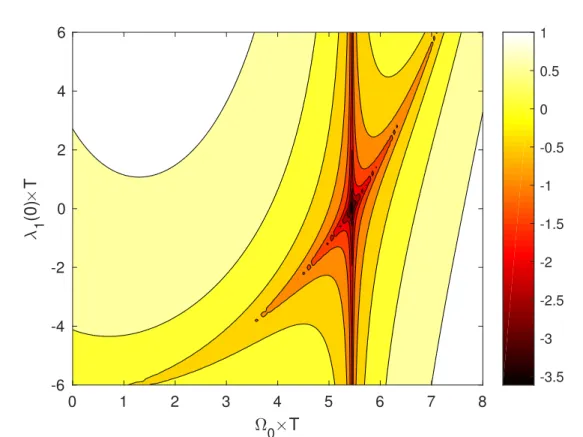
3.1 Decimal logarithm of the deviation " for various Ω0T and 1(0)T for

!= ⇡/2T . . . 43

3.2 Parameters ' and ✓ (in units of 1/T ) corresponding to Eq. (3.159) (↵ = 36) (full lines) and Eq. (3.160) ( = 2) (dashed lines), respectively, as function of time. . . 47

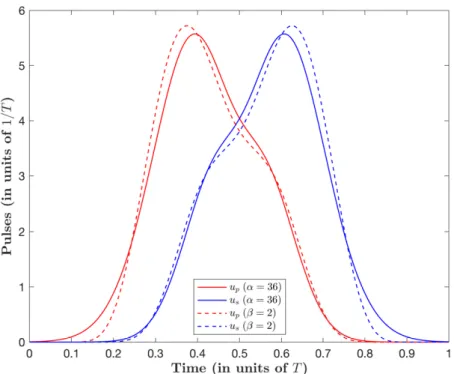
3.3 Control pulses up and us (in units of 1/T ) corresponding to Eq. (3.159)

(↵ = 36) (full lines) and Eq. (3.160) ( = 2) (dashed lines), respectively, as function of time. . . 47

3.4 Schematic representation of a control amplitude uk(t), consisting of N

discretization steps of duration ∆t = T /N. During each step n, the control amplitude uk,n is constant. The vertical arrows represent the

gradients of J, indicating how each amplitude uk,n should be modified in

the next iteration to improve the cost J. . . 50

3.5 Curve of the minimum energy with the variation of 3 for a given value

(11)

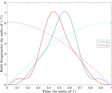
3.6 Pump up (solid blue line) and Stokes us (solid red line) pulses with the

parameters 1 = 0.3964, 3 = 0.1850, #1 = 0.9560 and #3 = 0.2220,

that gives the smallest energy for a given A = 0.0879T in the chosen 8-parameter restricted space, compared to the pump (dashed cyan line) and Stokes (dashed magenta line) pulses derived by linear multi-mode driving. . . 60

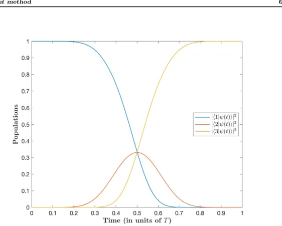
3.7 Dynamics of the populations resulting from pulses (solid lines) of Figure 3.6. The transfer from state |1i to state |3i is exact due to the chosen boundaries (STIREP). . . 61

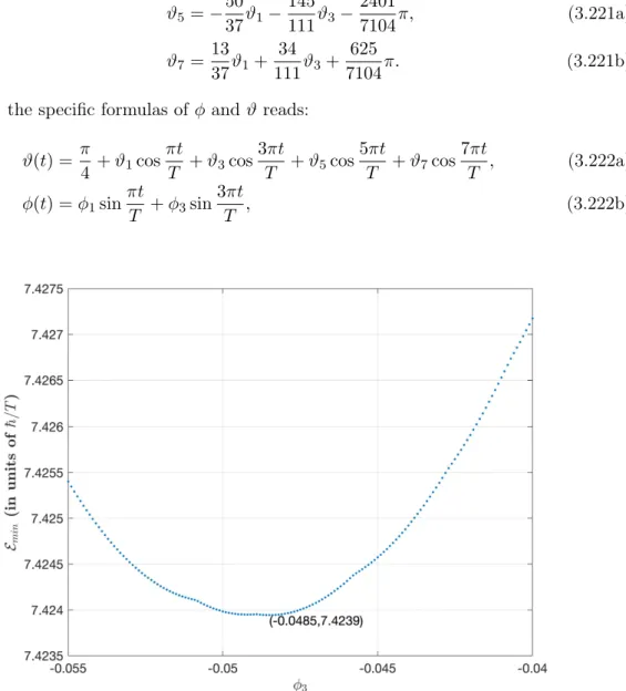
3.8 Curve of the minimum energy with the variation of 3 for a given A =

0.3750T ensuring the minimum energy in the 6-parameter space. . . 62

3.9 Pump up (solid blue line) and Stokes us (solid red line) pulses with the

parameters 1 = 0.9874, 3 = 0.0485, #1 = 0.9030, #3 = 0.1330

realizing the minimum energy in the 6-parameter space, compared to the pump (dashed cyan line) and Stokes (dashed magenta line) pulses derived from (3.155). . . 63

3.10 Populations resulting from pulses (solid lines) of Figure 3.9. . . 64

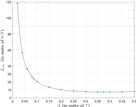
3.11 Dependence of the minimum energy on the time area of the transient population in the excited state. . . 64

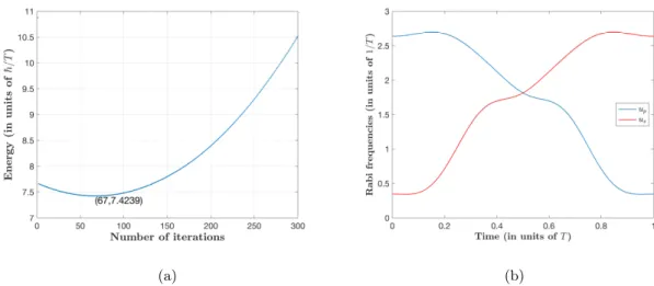
3.12 (a) Energy optimization using the gradient method from initial conditions close to the known minimum energy (with the parameters 1 = 1, 3 =

0.2, #1 = 0.8, #3 = 0.1, " = 0.00001). (b) Pump up (solid blue line)

and Stokes us (solid red line) pulses obtained from the optimization by

the gradient method (at the 101th iteration).. . . 67

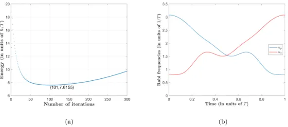
3.13 (a) Energy optimization using the gradient method from initial conditions very close to the known minimum energy (with the parameters 1 = 1, 3 = 0.2, #1 = 0.9030, #3 = 0.1330, " = 0.00001). (b) Pump up

(solid blue line) and Stokes us (solid red line) pulses obtained from the

optimization by the gradient method (at the 67th iteration). . . 68

4.1 Dependence of the optimal energy on the time area of the transient pop-ulation in the excited state. . . 86

4.2 Time-dependence of the parameters ' (upper frame, solid cyan line) and ✓ (upper frame, solid magenta line) (in units of 1/T ), the control pulses up (middle frame, solid red line) and us (middle frame, solid blue line)

(in units of 1/T ) and populations (lower frame) for the time area of the population in the excited state A = 3T /8 corresponding to unconstrained optimal pulses. . . 87

(12)

List of Figures vii

4.3 Same as Figure 4.2 but for A = 0.2T .. . . 88

4.4 Same as Figure 4.2, but for A = 0.07T .. . . 89

4.5 Controls for various values of A = 3T /8, A = 0.3T and A = 0.25T . . . . 90

4.6 Same as Figure 4.5 but for A = 0.2T , A = 0.15T and A = 0.1T . . . 90

4.7 Controls for A = 0.08T . The pump and Stokes controls appear as over-lapping pulses at the scale of the figure for A . 0.08T . . . 91

4.8 Controls for various values of A < 0.08T . . . 91

4.9 Comparison of the dynamics between (a) the energy-optimal STIREP and (b) the standard STIRAP featuring the same time area in the excited state A ' 0.036T .. . . 94

4.10 Time-dependence of dynamics for Ω0 = 14.453/T . Upper frame: The control pulses uP(t) and uS(t) (in units of 1/T ) according to (4.114). Middle frame: Populations with (t) the state solution. Lower frame: The eigenvalues given by (4.108) (in units of 1/T ). . . 96

4.11 Contour plots of solution(s) of '0 from Eq.(4.153) as a function of ˜µ and ˜_✓_{. Absence of solutions is indicated in black.} _{. . . 108}

4.12 Contour plots of logarithm to the base 10 of the absolute values of the difference between '(⇡/4) (from Eq. (4.151b)) and '0(from Eq. (4.153)), as a function of ˜µ and ˜✓ for (a) ˜µ  8; and (b) ˜µ 2] 8, 1]. . . 109

4.13 Dependence of the parameter ˜✓ on parameter ˜µ obtained from Table 4.3.112 4.14 Dependence of the optimal control time T on the area A obtained from Table 4.4. . . 114

4.15 Time-dependence of the parameters ' (upper frame, solid cyan line) and ✓(upper frame, solid magenta line), the control pulses up (upper middle frame, solid red line) and us (upper middle frame, solid blue line) (in units of u0), the projection (in absolute value squared) of the dynam-ics onto the dark state defined with the actual ✓ (lower middle frame), and populations (lower frame) for ˜µ = 0 and the resulting optimal time T = 2.72/u0 shown in Table 4.4 corresponding to unconstrained optimal pulses. . . 117

4.16 Same as Figure 4.15, but for ˜µ = 5. . . 118

4.17 Same as Figure 4.15, but for ˜µ = 10.5. . . 119

4.18 Same as Figure 4.15, but for ˜µ = 20.5. . . 120

4.19 Same as Figure 4.15, but for ˜µ = 24. . . 121

4.20 Comparison of the controls (in units of u0) for various couples of (˜µ, ˜✓) and the corresponding optimal time T from Table 4.4. . . 122

(13)

4.21 Same as Figure 4.20 but for larger negative values of ˜µ and the corresop-nding ˜✓ and optimal time T from Table 4.4. . . 122

4.22 Controls (in units of u0) for ˜µ = 11, ˜✓ = 6.2826117 and optimal time

T = 5.06/u0 from Table 4.4. . . 123

4.23 Controls (in units of u0) for ˜µ = 15, ˜✓ = 7.460490528 and optimal

time T = 5.96/u0 from Table 4.4. . . 123

4.27 Controls (in units of u0) for ˜µ = 24, ˜✓ = 9.581657691415900 and

optimal time T = 7.62/u0 from Table 4.4. . . 125

4.28 Pulse amplitudes for the three examples (i), (ii), (iii) described in the text. For (ii) and (iii), we have only plotted u0. . . 126

4.29 Final population transfer as a function of the deviation " for energy-optimal dissipative STIREP with respect to various time area of the transient population in the excited state A = 0.375T (unconstrained case) (solid blue line), A = 0.1T (solid red line) and A = 0.05T (dashed green line), respectively. . . 127

4.30 Comparison of final population transfer as a function of the deviation " between time-optimal dissipative STIREP (solid lines) and STIRAP (dashed lines) with respect to various time area of the transient popula-tion in the excited state A = 0.375T (unconstrained case) (blue lines), A = 0.1T (red lines) and A = 0.05T (green lines), respectively. . . 128

4.31 Stokes us (upper frame, solid red line) and Pump up (upper frame, solid

black line) (in units of 1/T ) for STIRAP, the projection (in absolute value squared) of the dynamics onto the dark state defined with the actual ✓ (middle frame) and the resulting populations with (t) the state solution (lower frame) in a situation of time area of the transient population in the excited state A = 0.375T . . . 129

4.32 Same as Figure 4.31 but for A = 0.1T . . . 130

4.33 Same as Figure 4.31 but for A = 0.05T . . . 130

5.1 Symbolic path diagrams giving the construction of the On integrals. The

symbol e stands for e(t), e0 for e(t0), and so on. For instance, for n = 3, the diagram features four paths. Its extension for larger n is direct. . . 135

(14)

List of Figures ix

5.2 Optimal robust trajectory e✓( ) corresponding to 1⇡ 1.1150 and 2 ⇡

0.3047 (leading to f = 5⇡/3).. . . 146

5.3 Time-dependence of Rabi frequency Ω (upper frame, solid blue line) and detuning ∆ (upper frame, solid red line) and the resulting populations Pj, j = 1, 2 (lower frame) for complete population transfer for the time

parameterization (t) (5.74). . . 147

5.4 Resulting detuning and dynamics of the populations Pj, j = 1, 2, for

robust time-optimal control [obtained for a flat pulse of Rabi frequency Ω0 according to (5.85)] showing the complete population transfer with

the optimal time Tmin⇡ 5.84/Ω0. . . 150

5.5 Optimal robust trajectory e✓( ) corresponding to 1⇡ 1.6974 and 2 ⇡

0.6465 (leading to f ⇡ 1.48⇡). . . 152

5.6 Time-dependence of Rabi frequency Ω (upper frame, solid blue line) and detuning ∆ (upper frame, solid red line) and the resulting populations Pj, j = 1, 2 (lower frame) for partial population transfer targeting the

half superposition state (up to a global phase). . . 152

5.7 Detuning and dynamics of the populations Pj, j = 1, 2, for robust

time-optimal control (for a flat pulse of Rabi frequency Ω0) showing the half

superposition. We obtain the optimal time Tmin ⇡ 4.05/Ω0. . . 153

5.8 Comparison of the robustness profile given by the RIO trajectories (solid cyan lines) with ⇡/2-pulse (solid magenta lines). Upper frame: Transition probability as a function of ↵. Lower frame: Logarithmic scale of the deviation targeting at half superposition state. . . 154

(15)

(16)

List of Tables

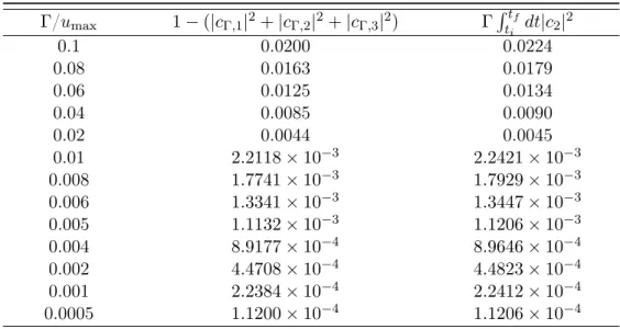
4.1 Losses of the model (4.1) (4.2a) and the approximate model (4.4) (4.2b) for different and relatively low ratios Γ/umax(obtained for example from

standard STIRAP with Gaussian pulses with the peak of the pulses set to umax= 6/T ). The approximate model provides reliable losses for the

ratio Γ/umax considered. . . 71

4.2 Optimal values of m, '0 and the corresponding energy E for various

A. The value A = 0.0879T corresponds to the multi-mode driving for k = 1 (see Section 2.4). The peak value umax and the pulse area A =

RT 0 ds

q u2

p+ u2s are also given. The pulse area for the Rabi frequency is

2A.. . . 84

4.3 Values of couple (˜µ, ˜✓) satisfying |'(⇡/4) '0| = 0, and the

correspond-ing values of log₁₀|'(⇡/4) '0|. . . 111

4.4 Resulting values of '0 (i.e. '(T /2)), the time area of the transient

pop-ulation in the excited state A and the optimal control time T for var-ious couples of (˜µ, ˜✓). The pulse energy E, Eq. (4.7), corresponds

to the value given for optimal time but in units of u0. The pulse area

A =R₀T dsqu2

p+ u2s is also given (which corresponds in fact to the value

(17)

(18)

Chapter 1

Introduction

With the continuous deepening of research on emergent quantum information pro-cessing, the manipulation of quantum systems has shown an increasing significance in quantum computing, quantum metrology, and high-resolution spectroscopy [1,2,3], and has brought tremendous changes and broad application prospects to the fields from laser spectroscopy, molecular and solid-state physics to nuclear magnetic resonance (NMR) and magnetic resonance imaging [4, 5, 6, 7, 8]. Thus achieving the manipulation of quantum systems, i.e., finding some achievable control fields to drive the controlled system evolving from the given initial state to the desired target state, plays an im-portant role in modern science and technology. Laser pulses are one of the most effec-tive methods to control the dynamics of quantum systems, and many techniques have been developed for such investigations, like resonant pulses, rapid adiabatic passage (RAP), stimulated Raman adiabatic passage (STIRAP) and the corresponding variants [9,10,11,12,13,14,15].

A well-known problem is to design solutions of quantum systems driven by external laser pulses that are optimal with respect to practical costs such as energy and duration [16]. The necessary conditions of optimality were established by Pontryagin via a max-imum principle [17]. Based on this approach, various optimal quantum problems have been solved from low- [18,19,20,21] to large-dimensional [22,8] systems. In a general sense, OCT is a optimal control method providing a direct optimization procedure, and is being widely valued by scientific researchers [23,24,25,26,27]. This corresponds to finding the optimal strategy, which allows the system to reach a specified target state while minimizing a given cost. There are two central steps in a typical workflow, first solving equations of motion resulting from the necessary condition of the PMP, and next selecting the optimal one(s) minimizing the cost. However, the practical application re-quires finding a simple and manageable representation of the problem (i.e. the relevant coordinates), which does not often yield closed-form formulas. Detailed calculation and examples will be presented in Chapters3 and4.

Solutions that additionally feature robustness have become a major issue in quantum physics, especially in quantum information processing, where ultra high-fidelity solutions

(19)

are required (typically with relative errors not above 10 4) [28]. Small imperfections in the design can cause fatal deviations of the performance. Robustness can be specifically taken into account using adiabatic [11, 12], composite [29, 30, 31], combined [32] or shortcut to adiabaticity (STA) [33, 34, 35, 36] techniques. However, these methods are not optimal and usually cost non-necessary energy and time. Combining robustness constraints with the optimization methods has thus become a major challenge [5]. OCT offers some solutions. More precisely, gradient method based on time discretization with thousands of parameters to be optimized [37] leads to very different results depending on the algorithm and the initial condition used, and rarely provides a global optimal solution. Alternative techniques involving from a few tens [38] to a few [39] parameters to be optimized have been developed, but they do not provide global optimal solutions in principle since they are based on restricted parametrizations. A recent proposal using Pontryagin’s maximum principle in an extended Hilbert space [40] allows an elegant integration of the robustness constraints, but leads to complicated systems to solve, only tractable for very simple targets, typically population transfers. A geometrical approach has been shown to provide optimal single-qubit phase gates [41]. All these methods use a direct optimization procedure, i.e. with the dynamical equations as constraints, which makes complicated the simultaneous integration of the robustness constraints. We next propose an alternative method of geometric optimization based on inverse engineering, mainly applying the single-shot shaped pulse method (SSSP) [35] for incorporating robustness, which we name robust inverse optimization (RIO). Details are presented in Chapter 5.

The present thesis is organized as follows:

In Chapter2 we present the invariant-based inverse engineering techniques contain-ing basic concepts, practical applications in two-/three-state systems and interpretations of exact passages from single-/multi-mode driving. We highlight that inverse engineer-ing techniques accelerate the process while simultaneously leadengineer-ing to an exact transfer via a trajectory determined by a choice of the time dependence of the parameters sat-isfying the appropriate boundaries. Applied to control in Λ systems, it is referred to as stimulated Raman exact passage (STIREP) in contrast to the approximate adiabatic passage of STIRAP.

In Chapter3we describe the general techniques of OCT, which allow one to obtain optimal trajectories in the parameter space. A general statement, basic approaches and involved concepts, such as the Lagrangian multiplier method, the Euler-Lagrange prin-ciple, the Pontryagin maximum principle (PMP), the shooting method and the gradient method are presented. Moreover, we show how PMP can be used to establish the formu-lation for low-dimension optimal quantum problems which can be solved analytically.

(20)

3

In Chapter4we apply PMP to determine solutions of a Λ three-state system driven by pump and Stokes pulses in a Raman configuration, which are optimal with respect to practical costs, including energy and duration, taking loss of the excited state into consideration. We first investigate the energy-minimum optimal control solution under a constraint of a given admissible loss in a fixed duration. We obtain the optimal controls featuring an intuitive pulse sequence for relatively large values of loss and a fully overlapping pulse sequence for small losses characterized by shorter duration and more intense amplitude. We next turn our attention to the problem of minimizing the time, still in such a three-state system, and obtain an intuitive shaping again for large losses. The optimal controls in the case of small losses show a transient counterintuitive pulse sequence resembling to the STIRAP sequence. The difference is that this transient counterintuitive sequence is sandwiched between fast intuitive sequences.

In Chapter 5, we take robustness into account. We develop a technique that allows the derivation of optimal and robust solutions achieving stipulated population transfer of two-state quantum systems. Instead of considering the dynamical equations of the problem as constraints of the optimization (as shown in Chapters3and4), we implement an inverse optimization: we determine in the independent dynamical variable space exact-fidelity trajectories constrained to robust solutions; the control fields are then derived from the obtained robust geodesics and the inverted dynamical equations where the parameters of the control fields are expressed as functions of the dynamical variables (that is the inverse-engineering representation of the Schrödinger equation). This RIO method is applied to design optimal control fields producing robust (complete and half) population transfers with respect to the pulse area. Such method can be applied to other quantum control problems such as quantum gates and other types of errors.

(21)

(22)

Chapter 2

From adiabatic passage to exact

passage: inverse engineering

techniques

Contents

2.1 Definition and properties . . . 6

2.2 Determination of the invariant . . . 9

2.2.1 Generalities . . . 9

2.2.2 Two-state system . . . 10

2.2.3 Three-state system . . . 11

2.3 Single-mode driving: From adiabatic to exact passage . . . 13

2.4 Multi-mode driving . . . 14

2.5 Disscussion . . . 19

One emblematic adiabatic passage technique is the stimulated Raman adiabatic passage (STIRAP), as shown in Figure2.1. It features a Λ quantum system driven by two-photon resonant pump and Stokes pulses, switched on and off in a counterintuitive sequence (first Stokes, next pump pulse, with a sufficient overlap). Such process, as all adiabatic processes, is based on the adiabatic theorem, which requires an infinite time of interaction (adiabatic limit). In practice they operate in a relatively long time in order to preserve a sufficient adiabaticity during the dynamics. As a consequence, adiabatic techniques, while in principle robust to systematic deviations of the parameters [13], are approximate and do not lead to exact transfer in a finite time.

For Raman systems, the upper state usually features dissipation (spontaneous emis-sion) and the STIRAP dynamics, in the adiabatic limit, follows an instantaneous dark eigenstate, which is immune to losses. However, in practice, operating in a finite time, the STIRAP process is lossy since it cannot follow exactly the dark state (see Section

2.3). Inverse engineering and other methods based on adiabatic techniques and compos-ite pulses [12,42,43,44] have been proposed to solve such issues, i.e., to accelerate the

(23)

process with an ultra-high fidelity and a robustness with respect to systematic errors. Finding an optimal compromise between fast, exact, immune to loss and robust process is still an open question, which we partially solve in this thesis.

In this chapter, we describe the invariant-based inverse engineering technique. It allows an exact transfer via a trajectory determined by a choice of the time dependence of the parameters satisfying the appropriate boundaries. This is referred to as stimulated Raman exact passage (STIREP) in contrast to the approximate adiabatic passage of STIRAP. Section 2.1 and Section 2.2 present some basic concepts of the invariant, in particular, Subsection 2.2.2 and Subsection 2.2.3 show the applications in two- and three-state systems, respectively. Exact passages are interpreted in Sections2.3and2.4

in terms of single-mode and multi-mode generalizing the eigenstate(s) approximately followed during an adiabatic dynamics. Discussion is provided in Section 2.5.

Figure 2.1: Diagram of a three-level Λ-type system for stimulated Raman processes at two-photon resonance. Ωp and Ωsdenote the pump and Stokes Rabi frequencies, which connect the initial ground state |1i and the excited state |2i, the excited state |2i and the final target state |3i, respectively.

2.1 Definition and properties

The Lewis-Riesenfeld dynamical invariant extends the concept of classical invariant to quantum mechanics [45]. It is formulated by an Hermitian operator I(t) whose quantum average is constant during the dynamics:

(24)

2.1. Definition and properties 7

I(t)| (t)i + h (t)|@I(t)

@t | (t)i + h (t)|I(t) ⇣ d

dt| (t)i ⌘

= 0, (2.2)

i.e., from _dtd_{h (t)| (t)i =} _dtd_{h (t)| | (t)i + h (t)|} _dtd_{| (t)i = 0 giving i}_dtd_{h (t)| =} h (t)|H, to

i@I

@t = [H(t), I(t)]. (2.3)

The eigenvectors | _{n(t)i of the invariant, with} n the eigenvalues,

I(t)| _{n(t)i =} n| n(t)i (2.4)

allow one to define a basis of dynamical modes on which we can expand the solution of the Schrödinger equation as

| (t)i =X n

cn,iei⇠n(t)_|

n(t)i (2.5)

with the connection at the initial time ti

cn,i= h n(ti)| (ti)i (2.6)

and the Lewis-Riesenfeld phases ⇠n(t) = Z t ti dsD n(s) i @ @s H(s) n(s) E . (2.7)

The invariant features the following properties: Its eigenvalues n are time independent.

We show it by considering the scalar product on (2.3):

iD m(t) @I @t n(t)

E

= ( n m)h m(t)|H(t)| n(t)i (2.8) and on the time derivative of (2.4):

D m(t) @I @t n(t) E = ( n m)h m(t)| @| _n(t)i @t + @ n @t mn. (2.9)

(25)

Considering m = n, or a degenerate eigenvalue, gives from (2.8) D n(t) @I @t n(t) E = 0 (2.10) and from (2.9) D n(t) @I @t n(t) E = @ n @t , (2.11)

from which we conclude @ n

@t = 0.

For _{m 6= n, one concludes, only if the eigenvalue is non-degenerate:} iD m(t)

@ @t n(t)

E

= h m(t)|H(t)| n(t)i. (2.12) The eigenvalues nare real and the eigenvectors | n(t)i form an orthonormal basis, i.e. _h _m(t)| _{n(t)i =} mn since I(t) is Hermitian.

If _{| (t)i is solution of the Schrödinger equation i}@_@t| i _{= H(t)| (t)i, then I(t)| (t)i} is also solution.

= H(t)I(t)| (t)i. (2.13)

To show (2.5)-(2.7), we use the spectral expansion

I(t) =X n

n| n(t)ih n(t)|, (2.14)

and calculate, defining cn(t) = h n(t)| (t)i, and using (2.13):

(26)

2.2. Determination of the invariant 9

cm(t) = cm,iei⇠m(t) _(2.15)

with the cm,i and the phase ⇠m(t) given by (2.6) and (2.7) respectively.

We remark that the density matrix ⇢(t) = | (t)ih (t)| is itself an invariant since it is solution of the Von Neumman Equation:

i@⇢

@t = [H(t), ⇢(t)]. (2.16)

2.2 Determination of the invariant

2.2.1 Generalities

We assume that the Hamiltonian has the general form H(t) =X

i

Ωi(t)Ti, (2.17)

where the set {Ti} of the N Hermitian and time independent operators T_i†= Tigenerates a close algebra:

[Ti, Tj] = X

k

C_ijkTk, Cjik = Cijk, Cijk = Cjki = Ckij . (2.18)

(27)

We seek for an invariant as an element of the algebra: I(t) =X

i

↵i(t)Ti. (2.19)

Since I(t) and the Ti’s are Hermitian, the ↵i(t)’s are real. We can calculate: i@ @tI(t) = i X i ˙↵iTi = [H(t), I(t)] =X ij Ωi(t)↵j(t)[Ti, Tj] =X ijk Ωi(t)↵j(t)CijkTk =X ijk Ωk(t)↵j(t)Ckji Ti. We then get the coefficients ↵i’s solution of the equation:

i ˙↵i = X j ij(t)↵j(t), ij(t) = X k Ωk(t)C_kji . (2.20)

The matrix B(t) = [ ij(t)]i=1..N,j=1..N is Hermitian (with purely imaginary elements) since ji(t) =PkΩk(t)Ckij =

P

kΩk(t)Ckji = ij(t). Denoting

|↵(t)i = [↵1(t), ↵2(t), · · · , ↵N(t)]T, (2.21) where the superscript T denotes the transpose of the vector, the equation reads:

id

dt|↵(t)i = B(t)|↵(t)i, B

†_{(t) = B(t).} _(2.22)

The propagator of this equation is then unitary, which implies: h↵(t)|↵(t)i =X

i

↵2_i_{(t) = const. = h↵(t}i)|↵(ti_)i. (2.23)

2.2.2 Two-state system

We consider the two-state system:

H = 1 2 " ∆ Ω Ω ∆ # = 1 2∆ z+ 1 2Ω x (2.24)

(28)

2.2. Determination of the invariant 11

with ∆ and Ω real. This corresponds to the SU(2) Lie algebra (N = 3) with

T1 ⌘ x/2, T2 ⌘ y/2, T3 ⌘ z/2, [T1, T2] = iT3 (2.25) (and all cyclic permutations of the indices), with Ω1= Ω, Ω2= 0, Ω3 = ∆, C123 = i and C₁₂k6=3= 0. The matrix B reads

B = 2 6 4 0 i∆ 0 i∆ 0 iΩ 0 iΩ 0 3 7 5 . (2.26)

To parametrize the three angles ↵i’s of the expansion (2.19), we need two (time-dependent) angles ', ✓ and a constant ↵0 in order to satisfy (2.23), ↵21+ ↵22+ ↵23 = ↵20:

↵1 = ↵0cos ' sin ✓, ↵2 = ↵0sin ' sin ✓, ↵3= ↵0cos ✓. (2.27) Equation (2.22) leads to

˙✓ = Ω sin ', ∆ = ˙' ˙✓ cotan ' cotan ✓, (2.28) which connects the angles (✓, ') to the pulse parameters (Ω, ∆). The invariant I(t) reads with the parametrization (2.27):

I(t) = ↵0 2

"

cos ✓ sin ✓e i' sin ✓ei' _{cos ✓}

#

, (2.29)

giving the dynamical modes and the associated phases

| _{1(t)i =} " cos(✓/2)e i'/2 sin(✓/2)ei'/2 # , 1= ↵0 2 , ˙⇠1 = Ω 2 cos ' sin ✓ = ˙✓ 2 cotan ' sin ✓ , (2.30a) | 2(t)i = " sin(✓/2)e i'/2 cos(✓/2)ei'/2 # , 2= ↵0 2 , ˙⇠2 = Ω 2 cos ' sin ✓ = ˙✓ 2 cotan ' sin ✓ . (2.30b) 2.2.3 Three-state system

We consider the (both one-photon and two-photon) resonant three-state system (in the rotating wave approximation):

H = ~ 2 2 6 4 0 Ωp(t) 0 Ωp(t) 0 Ωs(t) 0 Ωs(t) 0 3 7 5 = ~₂(Ωp(t)K1+ Ωs(t)K2) (2.31)

(29)

with Ωp and Ωs real, where K1, K2, and K3 are angular-momentum operators for spin 1: K1 = 2 6 4 0 1 0 1 0 0 0 0 0 3 7 5 , K2 = 2 6 4 0 0 0 0 0 1 0 1 0 3 7 5 , K3= 2 6 4 0 0 i 0 0 0 i 0 0 3 7 5 , (2.32) satisfying the commutation relations

[K1, K2] = iK3, [K2, K3] = iK1, [K3, K1] = iK2. (2.33) This corresponds to the SU(2) Lie algebra (N = 3) with

T1 _{⌘ K}1, T2 _{⌘ K}2, T3 _{⌘ K}3, [T1, T2] = iT3 (2.34) (and all cyclic permutations of the indices), with Ω1 = Ωp, Ω2 = Ωs, Ω3 = 0, C₁₂3 = i and C₁₂k6=3= 0. The matrix B reads

B = ~ 2 2 6 4 0 0 iΩ2 0 0 iΩ1 iΩ2 iΩ1 0 3 7 5 . (2.35)

To parametrize the three angles ↵i’s of the expansion (2.19), we need again two (time-dependent) angles ', ✓ and a constant ↵0 in order to satisfy (2.23), ↵21+ ↵22+ ↵23= ↵20:

↵1 = ↵0sin ✓ cos ', (2.36a)

↵₂ = ↵0cos ✓ cos ', (2.36b)

↵₃ = ↵0sin '. (2.36c)

Equation (2.22) allows one to write the Rabi frequencies as functions of angles (✓, '):

Ω1/2 ⌘ Ωp/2 = ˙'cos ✓ + ˙✓ sin ✓ cotan ', (2.37a) Ω2/2 ⌘ Ωs/2 = '˙sin ✓ + ˙✓ cos ✓ cotan '. (2.37b) The invariant I(t) reads with the parametrization (2.36a):

I(t) = ↵0 2 6 4

0 sin ✓ cos ' i sin ' sin ✓ cos ' 0 cos ✓ cos '

i sin ' cos ✓ cos ' 0 3 7

(30)

2.3. Single-mode driving: From adiabatic to exact passage 13

giving the dynamical modes and the associated phases

| _{0(t)i =} 2 6 4 cos ✓ cos ' i sin ' sin ✓ cos ' 3 7 5 , 0= 0, ˙⇠0= 0, (2.39a) | _{±(t)i =} _p1 2 2 6 4

cos ✓ sin ' ± i sin ✓ i cos ' sin ✓ sin ' ± i cos ✓

3 7

5 , ±= ±↵0, ˙⇠±= ⌥ ˙✓

sin '. (2.39b)

2.3 Single-mode driving: From adiabatic to exact passage

We consider the passage from the initial state |1i to the target state |3i in the three-state problem. Adiabatic passage assumes a slow evolution of the parameters such that adiabatic theorem applies: the dynamics is achieved approximately along a single adiabatic state, which connects the initial with the final states. In the three-state system, the considered adiabatic state is the well-known dark state

| D(t)i = 2 6 4 cos ✓ 0 sin ✓ 3 7 5 , (2.40)

where ✓ is the mixing angle, tan ✓ = Ωp/Ωs. We emphasize that the dynamical mode (2.39a_{) corresponds to the dark state for ' = 0. The initial state |1i can in principle}

connect to the dark state in a counterintuitive sequence, i.e. when the Stokes precedes the pump pulse (i.e. ✓ going from 0 to ⇡/2), but the dynamics cannot permanently project exactly on it since the dark state is connected to the other adiabatic states through the non-adiabatic coupling. This coupling can be made small only for a slow variation of the parameters (adiabatic passage), which corresponds to a small value of '. The Lewis-Riesenfeld invariant allows one to derive an alternative dynamical exact basis, on which one can project the dynamics exactly from the initial condition to a desired target state. The dark state can thus be interpreted as an approximation of the mode | _{0(t)i. Accelerating the dynamics along this mode will necessarily induce} population on the lossy excited state (through the component i sin ').

One can for instance impose a single-invariant-mode driving by imposing at the ini-tial time ✓(ti) = 0 and '(ti) = 0, with the final boundary ✓(tf) = ⇡/2 and '(tf) = 0 at time tf, which then drives the dynamics into the target state. These boundaries have to be taken into account in the definition of the pulses (2.37) to ensure the desired transfer. Such a single-mode dynamics can be interpreted as an exact passage compared to the

(31)

adiabatic passage occurring approximately along the dark state. Keeping the bound-aries, we still have the freedom to choose any time dependent shape of the angles ✓(t), '(t). For instance, the dynamics can also feature a speed up with respect to adiabatic passage or a certain degree of robustness by an appropriate time parametrization of the angles ✓(t) and '(t). In Ref. [35], a recipe is provided to derive robust pulse in two-level systems. In Ref. [36], it is analyzed for Λ systems. Specific optimizations can also guide the shaping as studied in the next chapters.

2.4 Multi-mode driving

One can determine other representations of the solutions, such as multi-mode solu-tions, which involve the three modes. We can choose for instance a multi-mode solution using ✓(ti) = 0, denoting the initial boundary '(ti) = 'i, according to (2.5):

| (t)i = c0| _{0(t)i + c+}ei⇠+(t)_| _{+(t)i + c e}i⇠ (t)_| _(t)i _(2.41)

with

c0= h 0(ti)|1i = cos 'i, (2.42a) c+= h +(ti)|1i = sin 'i/

p

2, (2.42b)

c = h (t_{i)|1i = sin 'i}/p2, (2.42c) and the Lewis-Riesenfeld phase ⇠0= 0 (since 0= 0).

For simplicity we consider the simple parametrization with t 2 [ti ⌘ 0, tf ⌘ T ]: '(t) = 'i, ✓(t) =

⇡

2Tt, (2.43)

giving the phase

⇠_{±(t) = ⌥⇠(t) = ⌥} ✓(t) sin 'i

. (2.44)

The probability amplitude in state |3i at time t reads

h3| (t)i = sin ✓(t)(cos2'i+ cos ⇠+(t) sin2'i) sin 'icos ✓(t) sin ⇠+(t), (2.45) which gives at final time

(32)

2.4. Multi-mode driving 15

The complete population transfer is then finally achieved when cos ⇠+(T ) = cos( ⇡ 2 sin 'i ) = 1, (2.47) i.e. sin 'i= 1 4k, k = ±1, ±2, ±3, · · · . (2.48) The resulting pulses

Ωp = ⇡ T p 16k2 _{1 sin}⇣ ⇡ 2Tt ⌘ , (2.49a) Ωs = ⇡ T p 16k2 _{1 cos}⇣ ⇡ 2Tt ⌘ , (2.49b)

feature a counterintuitive sequence. The smallest pulse energy required for the complete transfer with such pulses is for k = ±1.

An important quantity that will be considered frequently in this work is the time area of the transient population in the excited state:

A = Z T

0 |h2| (t)i|

2_. _(2.50)

It will indeed characterize with a good approximation of the loss in the Raman system during the process through the lossy upper state, see Section 4.1. We determine its value for this multi-mode driving:

A = T cos2'_isin2'_ih3 2 + sin 'i ⇡ ⇣1 2sin ⇡ sin 'i 4 sin ⇡ 2 sin 'i ⌘i . (2.51) We show in Figure2.2_{the corresponding dynamics for k = 1, giving A ' 0.0879T , and}

in Figure 2.3_{for k = 2 giving A ' 0.0231T . One can notice that the number of peaks}

of P2(t) is given by k.

One can remark that this dynamics with such pulses can be reinterpreted as a single-mode dynamics with different angles ✓ and ' (and the required boundary conditions ✓(ti) = 0, '(ti) = 0, ✓(tf) = ⇡/2, '(tf) = 0) given by

cos ' cos ✓ =⇥1 + sin2'i cos ⇠(t) 1 ⇤cos(⇡t/2T ) + sin 'isin ⇠(t) sin(⇡t/2T ), (2.52a)

sin ' = cos 'isin 'i 1 cos ⇠(t) , (2.52b)

cos ' sin ✓ =⇥1 + sin2'_i cos ⇠(t) 1 ⇤sin(⇡t/2T ) sin 'isin ⇠(t) cos(⇡t/2T ), (2.52c) with (2.44): ⇠(t) = ✓(t)/ sin 'i. The curves of ✓ and ' for k = 1 are shown in Figure

(33)

Figure 2.2: Pump Ωp (upper frame, solid red line) and Stokes Ωs (upper frame, solid blue line) (in units of 1/T ) and the resulting populations with (t) the state solution (lower frame) for k = 1.

(34)

2.4. Multi-mode driving 17

Figure 2.3: Pump Ωp (upper frame, solid red line) and Stokes Ωs (upper frame, solid blue line) (in units of 1/T ) and the resulting populations with (t) the state solution (lower frame) for k = 2.

(35)

Figure 2.4: Time-dependence of the parameters ' (upper frame, solid cyan line) and ✓ (lower frame, solid magenta line) (in units of 1/T) determined from Eq. (2.52) for k = 1.

(36)

2.5. Disscussion 19

2.5 Disscussion

In this chapter, we have shown that the Lewis-Riesenfeld invariant allows the deriva-tion of a mode that can be interpreted as an exact version of the well-known dark state leading to adiabatic passage (STIRAP). This mode induces an exact transfer instead of adiabatic and approximate and has to be considered in an inverse engineering procedure: choosing the dynamics of the angles that generate it and taking the appropriate bound-aries lead to the pulse shapes that ensure an exact transfer. This transfer is referred to as stimulated Raman exact passage (STIREP). We emphasize that, as expected, this mode that leads to an exact transfer features a non-zero transient component in the excited state contrary to the dark state.

Such transient population in the excited state is important to minimize since it will lead in practice to loss due to spontaneous emission. We expect typically coun-terintuitive pulse sequences (first Stokes, next pump) to do so. We have derived a simple (counterintuitive) sin / cos solution using a simple linear parametrization of the angles in a multi-mode configuration (that can be reinterpreted as a more complicated mono-mode solution). This solution is interesting since it is the opposite sequence of the one (intuitive cos / sin) that is the optimal solution minimizing the pulse energy E = ~₄R₀T(Ω2p + Ω2s)ds = 3⇡

2

4 ~

T (see Section 3.6). In that case, the optimal intuitive sequence is thus fast (in fact the fastest one for given peak pulses) but leads to a large transient population in the excited state, which can be characterized by its time area: A =R₀Tsin2'_{(t)dt ' 0.3750T , and is thus subject to loss in practice. The} counterintu-itive sin / cos sequence that we have derived is slower (but exact) and requires five times more energy E = ~₄R₀T(Ω2p+ Ω2s)ds = 15⇡

2

4 ~

T but gives four times smaller population in the excited state A ' 0.0879T . Optimization including losses is the subject of Chapter

(37)

(38)

Chapter 3

Techniques of optimal control in

quantum systems

Contents

3.1 Introduction . . . 22

3.2 Lagrange multiplier method . . . 23

3.2.1 Description of the method . . . 23

3.2.2 Example. . . 25

3.2.3 Extension of the method for a time-dependent constraint . . . 27

3.3 Euler-Lagrange principle . . . 28

3.4 The Pontryagin maximum principle . . . 31

3.4.1 The Lagrangian problem with constraints and controls . . . 32

3.4.2 The PMP for the Mayer problem . . . 33

3.4.3 The PMP for the Mayer-Lagrange or Lagrange problems. . . 34

3.5 Optimal control with constrained controls . . . 36

3.6 Maximum Principle and shooting method for the three-level problem . . . 38

3.6.1 Original coordinates . . . 38

3.6.2 Spherical coordinates. . . 42

3.7 Optimal Control by gradient method . . . 48

3.8 Trigonometric expansion for finite-time stimulated Raman ex-act passage (STIREP) by gradient method . . . 56

3.8.1 Counterintuitive sequence as a starting point in a 8-parameter space 56

3.8.2 Intuitive sequence . . . 61

3.8.3 Gradient method . . . 65

Optimal control problems of quantum systems can be outlined as seeking extremum solutions with respect to given costs. Generally, from a mathematical model represented typically by a differential equation, and additional constraints, one has first to formulate

(39)

appropriate objective functions which depend on actual demands such as the shortest control time, the smallest control field energy, or other optimal values of certain variables [18, 46]. Optimal control techniques allow one to obtain optimal trajectories in the parameter space.

Section3.1gives the introduction and formulation of optimal control problems in the general form, of the Mayer-Lagrange type. Section3.2presents the Lagrange multiplier method for finding the extremums of functions with constraints. Section 3.3 presents the Euler-Lagrange principle for finding the optimal trajectory with fixed initial and final boundaries. Section 3.4 states the Pontryagin maximum principle (PMP), which is expressed according to three typical problems. In Section 3.5, we consider the opti-mization of constrained controls, used for instance for problems of time miniopti-mization. Section 3.6 describes the specific analysis of the techniques of optimal control theory applied to a three-level Λ-system. We present the gradient method in Section 3.7 to manage the optimal control by iterative algorithms and numerical analyses. Section3.8

shows a practical example of application of the gradient method to the quantum control of Λ systems.

3.1 Introduction

We consider the general control problem of the Mayer-Lagrange (or Bolza) type [18,47]: 8 > < > : J(x, u) = g x(tf), tf + Rtf ti f0 x(t), u(t), t dt, ˙x(t) = f x(t), u(t), t , x(ti) = xi, (3.1)

which consists in finding m external controls u(t) 2 Rm driving a dynamical system ˙x(t) = f x(t), u(t), t of trajectory x(t) 2 Rn_{with the initial condition x(t}

i) = xi, which minimizes the cost J, defined by a terminal condition g x(tf), tf , which describes a property of the state x(tf) at final time tf, e.g. its distance from a chosen target state, and a chosen function f0 taken into account via an integral:

u = arg

v min J(x, v) . (3.2)

The Mayer-Lagrange problem features a free final state in its general formulation. When the final point of the trajectory is fixed, x(tf) = xf, one has to consider additionally g x(tf), tf = 0 in the cost, which is referred to as a Lagrange problem [18].

(40)

3.2. Lagrange multiplier method 23

(with a free final state): J x(tf) = g x(tf), tf .

As an example, minimizing the energy corresponds to f0 x(t), u(t), t = ⌘||u||2, where ⌘ > 0 expresses a compromise between the goal of transferring the state according to g x(tf) and the goal of keeping the energy of the controls small. Minimizing the time to reach a given target state from a given initial state corresponds to f0 = 1.

A Mayer (or Mayer-Lagrange) problem can be transformed into a Lagrange problem and, conversely, a Lagrange problem into a Mayer problem (see below, in Section3.4).

3.2 Lagrange multiplier method

3.2.1 Description of the method

The Lagrange multiplier method addresses the optimization problem of finding the extremum of a function g(x), x 2 Rn_{under the constraint f (x) = 0 (first assumed scalar} for simplicity, i.e. f 2 R): ₍

J(x) = g(x),

f (x) = 0. (3.3)

In such problems, no dynamics is considered, time can be omitted. The extremum means that _@x@g

i = 0 for all xi, i = 1, · · · , n, if the xi are all independent. But the constraint

introduces a dependence between the xi: one can express one xj as a function of the n 1 other xi; choosing j = n: xn= xn(x1, · · · , xn 1), (3.4) i.e. dxn= @xn @x1 dx1+ · · · + @xn @xn 1 dxn 1. (3.5)

We plug this relation into dg = _@x@g

1dx1+ · · · + @g @xndxn: dg =⇣ @g @x1 + @g @xn @xn @x1 ⌘ dx1+ · · · +⇣ @g @xn 1 + @g @xn @xn @xn 1 ⌘ dxn 1, (3.6) leading to @g @xi + @g @xn @xn @xi = 0, i = 1, · · · , n 1, (3.7) since g is extremum dg = 0. We also have an equivalent relation for f since f = 0:

@f @xi + @f @xn @xn @xi = 0, i = 1, · · · , n 1, (3.8)

(41)

i.e. @xn @xi = @f @xi ⇣ @f @xn ⌘ 1 . (3.9)

Combining with the expression (3.7) leads to @g @xi @g @xn @f @xi ⇣ @f @xn ⌘ 1 = 0, i = 1, · · · , n 1, (3.10) i.e. @g @xi @f @xi = @g @xn @f @xn , i = 1, · · · , n 1. (3.11)

We define the constant Lagrange multiplier ensuring the preceding equality (3.11) for all xi [48]: = @g @xn ✓ @f @xn ◆ 1 , i.e. @g @xn + @f @xn = 0. (3.12)

The resulting equations that have to be solved read thus: @g

@xi

+ @f @xi

= 0, i = 1, · · · , n. (3.13)

One can reformulate it using a Lagrangian

L = g + f, (3.14)

and one has to solve (3.13): @L @xi = 0, @L @ = f = 0, (3.15) corresponding to solving @L @qi = 0, i = 1, · · · , n + 1 (3.16)

for the augmented system of vectorial coordinate q = [xT_{, ]}T_.

If there are several constraints, i.e. f is a vector, one has to consider a Lagrange multiplier i for each constraint, leading to a vector of the same dimension of f . The Lagrangian reads then:

L = g + T_f _(3.17)

with the scalar product T_{f =}P

(42)

3.2.2 Example

As an interesting and simple example [49], we can consider the problem of finding the extremum of a quantum mean value hAi|Ψi of an observable A in a state

|Ψi = N X

i=1

ai_|ii, (3.18)

expanded in the basis {|ii, i = 1, · · · , N}. The constraint is the quantum normalization: N

X i=1

|ai|2 = 1. (3.19)

We have thus to find the extremum of

g(a1, a2, · · · , aN, a⇤1, a⇤2, · · · , a⇤N) := hAi|Ψi = X

i,j

a⇤_iajhi|A|ji, (3.20)

i.e., the components {ai} of the state which lead to the extremum (minimum or maxi-mum of g) under the constraint (3.19) which also reads

f := N X

i=1

aia⇤i 1 ⌘ 0. (3.21)

The Lagrange multiplier method shows the following equations according to (3.13): @g @a⇤ n + @f @a⇤ n = 0, (3.22a) @g @an + @f @an = 0, (3.22b)

in which, is the Lagrange multiplier and the other components can be obtained from (3.20) and (3.21): @g @a⇤ n = N X j=1 a_jhn|A|ji, @f @a⇤ n = an, @g @an = N X i=1 a⇤_i_hi|A|ni, @f @an = a⇤_n. (3.23)

We remark that, in this problem, we have considered for convenience the two sets of variables ai, a⇤i instead of the real and imaginary parts of the ai’s. This is possible since

(43)

is real as shown below (see Eq. (3.25)). Hence, (3.22) becomes N X i=1 a_{ihn|A|ii + an}= 0, (3.24a) N X i=1 a⇤_i_{hi|A|ni + a}⇤_n= 0, (3.24b)

that is, if is real,

A 2 6 6 4 a1 .. . aN 3 7 7 5 = 2 6 6 4 a1 .. . aN 3 7 7 5 , (3.25)

which corresponds to an eigenvalue problem. Since A is hermitian, the eigenvalues ⌘ are real, which is compatible with the passage from (3.24) to (3.25):

A 2 6 6 4 a1 .. . aN 3 7 7 5 = 2 6 6 4 a1 .. . aN 3 7 7 5 . (3.26)

We remark that, according to the method, all the eigenvalues give an extremum solution. Eq. (3.24) can be simply rewritten as:

N X

i=1

a_{ihn|A|ii =} an⌘ an. (3.27)

Plugging (3.27) into (3.20), we obtain

hAi|Ψi =X i a⇤_iX j aj_hi|A|ji =X i a⇤_i ai = X i |ai|2 = , (3.28)

which means that the absolute maximum (minimum) value of a quantum mean value hAi|Ψi is the maximum (minimum) value of the eigenvalues of A, realized by the state |Ψi being the corresponding eigenstate. One concludes that applying the Lagrange multiplier method transforms the problem of finding the extremum of a quantum mean

(44)

value of an operator A into the one of finding the extremum of the eigenvalue of A.

3.2.3 Extension of the method for a time-dependent constraint

If we consider the extremum of a function g(x) with a time-dependent vectorial constraint of the type

f x(t), ˙x(t), t = 0, _{t 2 [ti}, tf], (3.29) we have to introduce a Lagrange multiplier vector of the dimension of f for each time t, i.e. the Lagrange multiplier vector becomes itself time dependent (t). The scalar product in (3.17) has to be extended to time via an integral and the Lagrangian L becomes:

L(x) = g(x) + Z tf

ti

T_{(t)f x(t), ˙x(t), t dt,} _(3.30) where g(x) is defined for convenience through a functional:

g(x) = Z tf

ti

L0 x(t), ˙x(t), t dt. (3.31)

We will consider typically the constraint as a first order differential equation:

˙x = f x(t), t (3.32) giving L(x) = Z tf ti L0 x(t), ˙x(t), t dt + Z tf ti T_(t)⇣ d dtx f x(t), t ⌘ dt. (3.33)

Application of the method leads to @L @x = 0,

@L

@ T = 0 (3.34)

The second equation allows one to recover the constraint ˙x = f (x, t). The first equation has to be applied after an integration by part.

L = Z tf ti dt L0 x(t), ˙x(t), t +⇥ T(t)x(t)⇤tf ti Z tf ti dt⇣˙Tx + T(t)f x(t), t ⌘ (3.35) giving @L @x = Z tf ti dt⇣@L0 @x ˙ T T@f @x ⌘ = 0. (3.36)

(45)

This gives the differential equations for the Lagrange multipliers, called costate [18]:

˙T₌ @L0 @x

T@f

@x. (3.37)

The problem introduced in Section 3.1can be formulated in similar way. We consider the dynamical problem (the constraint):

˙x = f x(t), u(t), t , x(ti) = xi (3.38) with m control variables u(t) minimizing a cost

J(x, u) = gf + Z tf

ti

f0 x(t), u(t), t dt (3.39) with gf a terminal condition and f0 a given function. In addition to the equation (3.34), we have to consider

@L

@u = 0, (3.40)

where L now writes: L(x, u) = gf+ Z tf ti f0 x(t), u(t), t dt + Z tf ti T_(t)⇣_˙x _{f x(t), u(t), t} ⌘_dt, _(3.41) which gives @f0 @u T_(t)@f @u = 0, (3.42)

which links the controls u to the costate . As formulated, the problem is difficult to solve since it needs to solve the differential (3.37) for the costate, which is in general at least of the same complexity of the original dynamical equation; for all the possible u(t). An approximate iterative algorithm is needed in general to find a local extremum and we have no guarantee that this extremum will be a (global) optimum. The alternative formulation using the Pontryagin maximum principle (see Section3.4) will allow one to find exact solutions for relatively simple problems.

3.3 Euler-Lagrange principle

The Lagrangian multiplier method for a time-dependent problem can be in fact reformulated and generalized with the Euler-Lagrange principle. The Euler-Lagrange principle corresponds to finding the trajectory x(t) of fixed boundaries x(ti) = xi and

(46)

3.3. Euler-Lagrange principle 29

x(tf) = xf, which realizes the extremum of the integral, defining the cost: J(x) =

Z tf

ti

L0 x(t), ˙x(t), t dt, (3.43)

where we recognize L0 as a Lagrangian and J the corresponding action in classical mechanics. The integral of the cost of (3.1) takes precisely this latter form. The Euler-Lagrange principle can be expressed by the Euler-Euler-Lagrange equations [50]

d dt @L0 @˙xi = @L0 @xi , (3.44)

which generalizes (3.14) to the dynamical case. The extremum trajectory x(t) is solution of the Lagrange equation (3.44), or equivalently of the Hamilton equations

˙xi = @H0 @pi , ˙pi= @H0 @xi (3.45) with the conjugate moment

pi = @L0

@˙xi

(3.46) and the Hamiltonian (with p a row vector)

H0= p ˙x L0. (3.47)

If the system is subject to a (vectorial) constraint (of the same type of the one in Lagrange multiplier method)

f x(t), ˙x(t), t = 0, (3.48)

one has to consider the augmented problem of coordinates q(t) = [x(t)T_, T_]T_{, which} features the modified Lagrangian:

L = L0 x(t), ˙x(t), t + Tf x(t), ˙x(t), t , (3.49) where the constraint is included via a real vector function = (t) of Lagrange multipliers having the same dimension of f , and called the costate in this con-text. We notice that we recover Eq. (3.30) of Subsection 3.2.3 with the connection L(x) =Rti

tf L0 x(t), ˙x(t), t dt. The Euler-Lagrange equations that have to be solved

d dt @L @˙qi = @L @qi , (3.50)

(47)

give for the Lagrange multiplier part d dt @L @ ˙ = 0 = @L @ = f, (3.51)

meaning that the constraint f = 0 is satisfied, and for the dynamical variables d dt @L0 @˙xi + Td dt @f @˙xi = @L0 @xi + T@f @xi . (3.52)

The latter can be rewritten as

grad J(x) + grad F (x) = 0, (3.53)

with the general definition of the gradient: grad Φ(x) = @' @x d dt @' @˙x, (3.54) for Φ(x) defined as Φ(x) = Z tf ti '(x, ˙x, t)dt. (3.55)

Here we have thus

F (x) = Z tf

ti

f (x, ˙x, t)dt. (3.56)

The Euler-Lagrange method generalizes thus the Lagrange multiplier method to con-straints and costs defined as functionals for dynamical problems.

If the constraint is a first order differential equation (with f having the same dimen-sion as x)

˙x = f (x, t), (3.57)

the Lagrangian becomes

L = L0(x, t) + T( ˙x f ), (3.58)

where L0(x, t) becomes only a function of x and t, and the equations to solve are given by the Euler-Lagrange equations

d dt @L @˙qi = @L @qi , (3.59) i.e. 0 = @L @ = ˙x f, (3.60)

(48)

3.4. The Pontryagin maximum principle 31

meaning that the constraint ˙x = f is satisfied, and d dt @L @˙x = ˙ T₌ @L @x = @L0 @x T@f @x, (3.61) i.e. ˙T₌ @L0 @x T@f @x, (3.62)

which represents the adjoint equation (of the costate). We recover Eq. (3.37) .

The problem can be reformulated by Hamilton equations with an Hamiltonian. The conjugate moments are by definition

px= @L

@˙x =

T_, _{p =} @L

@ ˙ = 0 (3.63)

with the corresponding Hamiltonian

H = T_˙x _{L =} T_f _L

0, (3.64)

and the Hamilton equations ˙x = @H @px = f, ˙px= ˙ T₌ @H @x = @L0 @x T@f @x. (3.65)

This shows that the conjugate moments are zero except the one associated to x, which is the Lagrange multiplier px= T _{and solution of Eq. (}_3.62_).

We remark that in this notation, the term @f_@x corresponds to a matrix, which reads for instance for n = 2:

@f @x = " _@f₁ @x1 @f1 @x2 @f2 @x1 @f2 @x2 # , (3.66) while @L0

@x is a row vector, i.e. for n = 2: @L0 @x =  @L0 @x1 ,@L0 @x2 . (3.67)

The problem is most often formulated with additional controls u(t), as in Eq. (3.1), and solved using the Pontryagin maximum principle [17] as shown below.

3.4 The Pontryagin maximum principle

(49)

3.4.1 The Lagrangian problem with constraints and controls

We consider the control problem (3.1). Following [18], we connect the Lagrangian L0 with f0 as

L0 x(t), u(t), t = p0f0 x(t), u(t), t , (3.68) with p0 a constant. The coordinates of the augmented problem are here q(t) = [x(t)T_{, u(t)}T_, T_]T_{; the equations of the dynamics are considered as the constraints,} and one remarks that the Lagrangian does not depend on ˙q. If {x, u} is an optimal solution of (3.1), then there exists a vector function = (t) of Lagrange multipliers such that {x, u, } is an optimal for the unconstrained problem of minimizing

L = L0+ T ⇣

˙x(t) f x(t), u(t), t ⌘. (3.69) The Euler equations read

d dt @L @˙x = ˙ T₌ @L @x = @L0 @x T@f @x, (3.70a) d dt @L @˙u = 0 = @L @u = @L0 @u T@f @u, (3.70b) d dt @L @ ˙ = 0 = @L @ = ˙x f, (3.70c) i.e., as before, ˙T₌ @L0 @x T@f @x, (3.71)

which represents the adjoint equation (of the costate), and @L0

@u = T@f

@u, (3.72)

which links u and . We notice that we recover Eq. (3.42) when p0 = 1. The conjugate moments are by definition

px = @L @˙x = T_, _p u = @L @˙u = 0, p = @L @ ˙ = 0 (3.73)

with the corresponding Hamiltonian

H = T˙x L = Tf L0= Tf p0f0, (3.74) and the Hamilton equations

˙x = @H @px = f, ˙px= ˙T= @H @x = p0 @f0 @x T@f @x. (3.75)

(50)

This shows that, as before, the conjugate moments are zero except the one associated to x which is the Lagrange multiplier px= T and solution of Eq. (3.71). The problem is solved using the Pontryagin maximum principle as shown below.

Remark: Multiplying the Hamiltonian by a constant ↵, ↵H = ↵pxf ↵p0f0, comes down to consider the couple (↵px, ↵p0), and leads to the same trajectory since ˙x =

@↵H @↵px = @H @px, ˙ (↵px) = ↵ ˙px = @↵H_@x = ↵@H_@x.

3.4.2 The PMP for the Mayer problem

We first formulate the Pontryagin maximum principle (PMP) on the Mayer problem [of free final state and a fixed final time is also considered: J x(tf) = g x(tf) ] [18], i.e. f0= 0 and, the adjoint equations of the costate and the Hamiltonian, read respectively:

˙T₌ T@f

@x, H =

T_f. _(3.76)

The PMP states that the Hamiltonian H is maximum (necessary conditions of optimal-ity) [17], i.e. @H @u = @ T_{f (x, u)} @u = T@f (x, u) @u = 0, (3.77)

for u satisfying the adjoint equation (3.76) with the terminal condition

T_(tf_{) =} @g

@x x(tf) , (3.78)

when there is no bound on the controls u.

To prove (3.77), we analyse a small variation of the control: u"(t) := u(t) + "v(t) and denote x"(t) the trajectory corresponding to u"(t). The corresponding variation of the cost reads

∆J := J x"(tf) J x(tf) ⇡ @g

@x x(tf) x"(tf) x(tf) , (3.79) which we can write as

∆J ⇡ _@x@g x(tf) z(tf)" = T(tf)z(tf)", (3.80) using the definition

z(t) := dx"(t)

d" (" = 0) (3.81)

(51)

to derive a differential equation for z: ˙z(t) = d ˙x"(t) d" (" = 0) = df x"(t), u(t) + "v(t) d" (" = 0) = @f x(t), u(t) @x z + @f x(t), u(t) @u v (3.82)

with initial condition z(ti) = 0. Considering the adjoint equation ˙T₌ T_(t)@f x(t), u(t)

@x , (3.83)

and the writing (since z(ti) = 0): T(tf)z(tf) = R_tt_if _dtd T(t)z(t) dt = R_tt_if ˙Tz(t) + T_{(t) ˙z dt, Eq. (}_3.80_{) can be rewritten as}

∆J ⇡ " Z tf

ti

T_(t)@f x(t), u(t)

@u v(t)dt. (3.84)

The necessary condition for u being a local minimum for J, i.e. ∆J = 0, correspond-ing to a local maximum for T_{(t)f x(t), u(t) , i.e. the Hamiltonian being maximum,} requires Eq. (3.77).

3.4.3 The PMP for the Mayer-Lagrange or Lagrange problems

If one has a Mayer-Lagrange (or Lagrange) problem instead of a Mayer problem, the conditions of the maximum principle can be adapted by transforming the problem into a Mayer problem. This is done by defining the extra (scalar) component y(t), which satisfies the constraint:

˙y = f0(x, u, t), y(ti) = 0. (3.85) Using this extra variable the cost takes indeed the Mayer form

J(u) = g x(tf), tf + y(tf). (3.86) The costate now has dimension n + 1. If we call the first n components of the costate and µ the remaining component, the adjoint equations take the form

˙T₌ T_(t)@f x(t), u(t)

@x µ

@f0 x(t), u(t)

@x , (3.87a)

(52)

with the additional terminal condition µ(tf) =

@ g(x, tf) + y

@y y(tf) = 1. (3.88)

This leads to the Hamiltonian

H = Tf + µf0 = Tf f0, (3.89)

which is maximum. As stated before, one can always for convenience consider the Hamiltonian multiplied by a (positive) constant ↵, ↵H = ↵ T_f _↵f0 _{with the same} trajectories x and . This means that we can always multiply f0 by a positive constant ↵ in the definition of the Hamiltonian (3.89). This constant ↵ changes the (as a multiplicative factor) but not the trajectory x(t), neither the optimum u.

To summarize, in order to derive solutions that satisfy the necessary conditions of optimality, we have to solve the system of equations

˙T₌ T_(t)@f x(t), u(t)

@x +

@f0 x(t), u(t)

@x , (3.90a)

˙x = f x(t), u(t) , (3.90b)

with the boundary conditions

x(ti) = xi, (3.91a)

T_(t f) =

@g

@x x(tf) , (3.91b)

such that the Hamiltonian

H = Tf + µf0= Tf f0 (3.92)

is maximum, i.e.

@H

@u = 0. (3.93)

This is a two points boundary value problem as the boundary conditions are at time ti and tf. The procedure of resolution is typically as follows: one leaves the initial condition for , (ti), as a free parameter, solves the equations (3.90) with the initial condition (3.91a), and then tries to adjust the value of the parameter (ti) so as to meet condition (3.91b). A typical method to implement this procedure is the shooting method (see below).