%0$503"5%&-6/*7&34*5² -6/*7&34*5²%&506-064& %&506-064&

%NVUEDELOBTENTIONDU

%0$503"5%&

%0$503"5%&-6/*7&34*5² -6/*7&34*5²%&506-064& %&506-064&

$ÏLIVRÏPAR $ISCIPLINEOUSPÏCIALITÏ

0RÏSENTÏEETSOUTENUEPAR

4ITRE

*529

%COLEDOCTORALE 5NITÏDERECHERCHE

$IRECTEURS DE4HÒSE

2APPORTEURS LE

Institut National Polytechnique de Toulouse (INP Toulouse)

Mécanique, Energétique, Génie civil et Procédés (MEGeP)

MODELING OF DIESEL HCCI COMBUSTION AND ITS IMPACT ON POLLUTANT EMISSIONS APPLIED TO GLOBAL ENGINE SYSTEM SIMULATION

mardi 2 février 2010

Alessio DULBECCO

Énergétique et Mécanique des Fluides

Olivier COLIN (Encadrant), François-Xavier DEMOULIN (Examinateur), Jean-François HETET (Examinateur), Pascal HIGELIN (Rapporteur), François-Alexandre LAFOSSAS (Examinateur), Angelo ONORATI (Rapporteur),

Thierry POINSOT (Directeur de thèse), Vincent TALON (Examinateur)

Pascal HIGELIN Angelo ONORATI

Thierry POINSOT Olivier COLIN IFP, CERFACS

Numéro d’ordre : ????

THÈSE

En vue de l’obtention du

DOCTORAT DE L’UNIVERSITÉ DE TOULOUSE

Délivré par : Institut National Polytechnique de Toulouse (INP Toulouse) Discipline : Énergétique et Mécanique des Fluides

Présentée et soutenue par Alessio DULBECCO le mardi 2 février 2010

TITRE

MODELING OF DIESEL HCCI COMBUSTION AND ITS IMPACT ON POLLUTANT EMISSIONS APPLIED TO GLOBAL ENGINE SYSTEM SIMULATION

JURY

Olivier COLIN Chargé de Recherche, IFP Encadrant IFP François-Xavier DEMOULIN Maitre de Conférences, Université de Rouen Examinateur Jean-François HETET Professeur, Centrale Nantes Examinateur Pascal HIGELIN Professeur, Université d’Orléans Rapporteur François-Alexandre LAFOSSAS Ingénieur de Recherche, Toyota Examinateur Angelo ONORATI Professeur, Politecnico di Milano Rapporteur Thierry POINSOT Directeur de Recherche, IMFT/CNRS Directeur de thèse Vincent TALON Ingénieur de Recherche, Renault Examinateur

École Doctorale : Mécanique, Énergétique, Génie civil et Procédés (MEGeP) Unités de recherche : IFP, CERFACS

Directeur de thèse : Thierry POINSOT

Rapporteurs : Pascal HIGELIN et Angelo ONORATI

Ai miei genitori Walter e Ornella e ai miei nonni Edo, Anna, Angelo e Maria

More and more stringent restrictions concerning the pollutant emissions of Internal Com- bustion Engines (ICEs) constitute a major challenge for the automotive industry. New combustion strategies such as Homogeneous Charge Compression Ignition (HCCI) and the implementation of complex injection strategies are promising solutions for achieving the imposed emission standards as they permit low NOxand soot emissions, via lean and highly diluted combustions, thus assuring low combustion temperatures. This requires the creation of numerical tools adapted to these new challenges. This Ph.D presents the development of a new 0D Diesel HCCI combustion model : the dual Combustion Model (dual−CM). The dual-CM is based on the PCM-FPI approach used in 3D CFD, which allows to predict the characteristics of Auto-Ignition and Heat Release for all Diesel combustion modes. In order to adapt the PCM-FPI approach to a 0D formalism, a good description of the in-cylinder mixture is fundamental. Consequently, adapted models for liquid fuel evaporation, mixing zone formation and mixture fraction variance, which allow to have a detailed description of the local thermochemical properties of the mixture even in configurations adopting multiple injection strategies, are proposed. The results of the 0D model are compared in an initial step to the 3D CFD results. Then, the dual-CM is validated against a large experimental database; considering the good agreement with the experiments and low CPU costs, the presented approach is shown to be promising for global engine system simulations. Finally, the limits of the hypotheses made in the dual-CM are investigated and perspectives for future developments are proposed.

Key words : Diesel HCCI Combustion, Fuel Evaporation, Probability Density Func- tions, Tabulated Complex Chemistry, 0D Model, Multiple Injection Sprays.

1

La législation sur les émissions de polluants des Moteurs à Combustion Interne (ICEs) est de plus en plus contraignante et représente un gros défi pour les constructeurs auto- mobiles.

De nouvelles stratégies de combustion telles que la Combustion à Allumage par Com- pression Homogène (HCCI) et l’exploitation de stratégies d’injections multiples sont des voies prometteuses qui permettent de respecter les normes sur les émissions de NO_x et de suies, du fait que la combustion a lieu dans un mélange très dilué et par conséquent à basse température.

Ces aspects demandent la création d’outils numériques adaptés à ces nouveaux défis.

Cette thèse présente le développement d’un nouveau modèle 0D de combustion Diesel HCCI : le dual Combustion Model (dual−CM). Le modèle dual-CM a été basé sur l’approche PCM-FPI utilisée en Mécanique des Fluides Numérique (CF D) 3D, qui per- met de prédire les caractéristiques de l’auto-allumage et du dégagement de chaleur de tous les modes de combustion Diesel. Afin d’adapter l’approche PCM-FPI à un formal- isme 0D, il est fondamental de décrire précisément le mélange à l’intérieur du cylindre.

Par consequent, des modèles d’évaporation du carburant liquide, de formation de la zone de mélange et de variance de la fraction de mélange, qui permettent d’avoir une descrip- tion détaillée des proprietés thermochimiques locales du mélange y compris pour des configurations adoptant des stratégies d’injections multiples, sont proposés.

Dans une première phase, les résultats du modèle ont été comparés aux résultats du modèle 3D. Ensuite, le modèle dual-CM a été validé sur une grande base de données expérimentales; compte tenu du bon accord avec l’expérience et du temps de calcul réduit, l’approche présentée s’est montrée prometteuse pour des applications de type simulation système. Pour conclure, les limites des hypothèses utilisées dans dual-CM ont été investiguées et des perspectives pour les dévélopements futurs ont été proposées.

Mots Clés : Combustion Diesel HCCI, Évaporation de Carburant, Fonctions de Densité de Probabilité, Tabulation de la Chimie Complexe, Modèle 0D, Jets d’Injections Multiples.

2

Abstract . . . 1

Résumé . . . 2

Nomenclature . . . 5

Chapter 1 Introduction . . . 12

1.1 The Diesel engine . . . 15

1.1.1 Principle of the four stroke Diesel engine . . . 16

1.1.2 The Common Rail system . . . 20

1.1.2.1 The multiple injection strategies . . . 22

1.1.3 The combustion process . . . 25

1.2 The global engine system study . . . 26

1.2.1 The global engine system test bench . . . 27

1.2.2 The global engine system simulation . . . 28

1.3 Objective and methodology . . . 29

Chapter 2 The dual Combustion Model (dual-CM) . . . 31

2.1 Context and model specifications . . . 32

2.2 Synoptical diagram of the model . . . 34

2.3 Injection rate model . . . 37

2.4 Spray model . . . 39

2.4.1 Evaporation submodel . . . 40

2.4.1.1 Fluid thermodynamic properties at liquid-gas interface . . 44

2.4.1.2 Liquid penetration length . . . 49

2.4.1.3 Fuel mass evaporation rate . . . 68

2.4.2 Gas entrainment submodel . . . 70

2.4.2.1 Injector orifice performance . . . 70

2.4.2.2 Gas entrainment modeling . . . 71

2.4.2.3 Extension of the model to multiple injection strategies . . 81

2.4.3 Turbulence submodel . . . 89

2.4.4 Mixture submodel . . . 92

2.5 Combustion model . . . 98

2.5.1 Tabulation of laminar combustion processes . . . 102

2.5.2 Laminar combustion submodel . . . 114 3

2.5.3 Turbulent combustion submodel . . . 123

2.6 Auxiliary models . . . 129

2.6.1 In cylinder gas mixture thermodynamic model . . . 129

2.6.2 Kinematic model of the piston motion . . . 132

2.6.3 Thermal loss model . . . 133

2.7 Parametric study of the model . . . 134

2.8 Computational time . . . 139

Chapter 3 Dual-CM engine validation . . . 144

3.1 Tested engine : Renault G9T NADI™concept engine . . . 144

3.1.1 The engine operating domain . . . 146

3.2 The 3D Computational Fluid Dynamics Code IFP-C3D . . . 146

3.3 Methodology for determining initial and boundary conditions . . . 150

3.4 Investigation of physical models using a comparison with a 3D code . . . . 154

3.5 Sensitivity of dual-CM to isoparametric variations . . . 162

3.6 Representative engine operating points of the experimental database . . . 165

3.7 Statistics on the entire engine operating domain . . . 168

Chapter 4 Limits and analysis of precision of dual-CM : investigation making a comparison with a 3D solver . . . 179

4.1 Influence of the combustion chamber shape on mixture formation . . . 180

4.2 The progress variable variance modeling . . . 189

Chapter 5 Conclusions and perspectives . . . 195

5.1 General conclusions . . . 195

5.2 Perspectives . . . 198

Appendix A The environment of simulation. . . 201

Appendix B ECFM3Z equations . . . 204

Appendix C The D² law . . . 207

Appendix D Variance equation proof . . . 217

Appendix E FPI trajectories in the phase space . . . 226

Appendix F Oil & Gas Science and Technology . . . 228

Appendix G SAE 2009-01-0678 . . . 255

Bibliography . . . 277

Acronyms

0D Zero Dimensional

1D One Dimensional

2D Two Dimensional

3D Three Dimensional

ACEA Automotive European Manufacturers’ Association ADF-PCM Approximated Diffusion Flame - PCM

AI Auto-Ignition

ALE Arbitrary Lagrangian Eulerian

ATDC After TDC

BDC Bottom Dead Center

BG Burned Gas

BTDC Before TDC

CFD Computational Fluid Dynamics CI Compression Ignition

CMC Conditional Moment Closure

CR Common Rail

CRS Common Rail System

DPF Diesel Particulate Filter dual-CM dual Combustion Model

ECFM3Z Three Zones Extended Coherent Flame Model ECU Electronic Control Unit

EGR Exhaust Gas Recirculation

EU European Union

EVC Exhaust Valve Closing EVO Exhaust Valve Opening

FIAT Fabbrica Italiana Automobili Torino FPI Flame Prolongation of ILDM

HCCI Homogeneous Charge Compression Ignition

HR Heat Release

HRR Heat Release Rate

5

ICE Internal Combustion Engine

ILDM Intrinsic Low-Dimensional Manifolds IVC Inlet Valve Closing

IVO Inlet Valve Opening

LAS Laser Absorption Spectrometry LIF Laser Induced Fluorescence LTC Low Temperature Combustion NADI Narrow Angle Direct Injection NTC Negative Temperature Coefficient

PCCI Premixed Controlled Compression Ignition PCM Presumed Conditional Moment

PDF Probability Density Function PIV Particle Image Velocimetry TDC Top Dead Center

VVA Variable Valve Actuator Latin abbreviations

a [m] crank radius

A [-] pure ambient air zone A(x) [m²] spray cross section area AV I [CAD] Injection Advance b [m] connecting rod length

B [-] transfer number at steady-state

B [m] bore

B_M [-] mass transfer number BT [-] thermal transfer number c [-] normalized progress variable C [mol/m³] molar concentration

C_a [-] orifice area contraction coefficient C_d [-] orifice discharge coefficient

c_v [J/kg/K] specific heat capacity at constant volume Cv [-] orifice velocity coefficient

cp [J/kg/K] specific heat capacity at constant pressure D [m²/s] laminar diffusion coefficient

D_d [m] drop diameter

d_h [m] injector orifice diameter dvc [m] vena contracta diameter

Dissip [J/m³/s] sensible enthalpy dissipation term

DT [s] Dwell Time

e [m] squish height

E˙ [1/s] mass transfer rate between zones

Ec [J] kinetic energy

EOC [CAD] End Of Combustion

EOI [CAD] End Of Injection

ET [s] Energizing time

F [-] pure fuel zone

F_i [N/m³] volumetric force h [J/kg] specific enthalpy

h⁰ [J/kg] formation enthalpy (computed at the temperatureT0) hc [W/m²/K] convective heat transfer coefficient

hs [J/kg] sensible enthalpy (referred to the temperature T0) IM EP [bar] Indicated Mean Effective Pressure

J [mol/m²/s] diffusion flux J_i^h [J/m²/s] enthalpy flow rate k [J/m/s/K] thermal conductivity K [J/kg] mean specific kinetic energy l [J/kg] fuel latent heat of vaporization L [m] fuel liquid penetration length

Le [-] non-dimensional spray liquid penetration

Le [-] Lewis’ number

m [kg] mass

m˙ [kg/s] mass flow rate through a spray cross section Ù˙

m [kg/s/m²] mass flow rate per surface unit

M [-] mixing zone

M [kg/mol] molecular weight M˙_Fl [N] spray momentum

m_tot [kg] total gaseous mass within the cylinder

n [mol] number of moles

ncyl [-] number of cylinders

n_h [-] number of injector orifices

p [Pa] pressure

P [-] single variable PDF

P_co [-] coupled PDF

p_vp [Pa] saturation pressure of the fuel p_x [Pa] partial pressure of the speciesx

P r [-] Prandtl’s number

Q˙^cb [J/s] combustion Heat Release Rate Q˙ev [J/s] fuel evaporation heat flow rate Q˙_hu [J/s] heat up heat flow rate

Q˙_th [J/s] thermal losses Q˙_tot [J/s] total heat flow rate

r [m] drop radius

R [J/kg/K] gas constant of the mixture R [J/mol/K] universal gas constant

s [-] mass stoichiometric coefficient

s [m] stroke

S [m] spray gaseous penetration S˙ [1/s] mass source term

Se [-] non-dimensional spray gaseous penetration S˙hs [J/kg/s] sensible enthalpy source term

S¯p [m/s] mean piston velocity S_w [m²] wall surface

Sc [-] Schmidt’s number

Sc_t [-] turbulent Schmidt’s number SM D [m] Sauter’s Mean Diameter SOC [CAD] Start Of Combustion SOI [CAD] Start Of Injection

t [s] time

T [K] temperature

et [-] non-dimensional time t⁺ [s] temporal length scale t_nod [s] needle opening delay

Tw [K] wall temperature

u [m/s] absolute velocity uB [m/s] Bernoulli’s velocity ur [m/s] radial convective velocity v [-] fuel mixture fraction variance V [m³] cylinder volume

V_b [m³] piston bowl volume V_d [m³] dead volume

V_displ [m³] piston displacement vr [m/s] radial diffusion velocity

W [J/m³/s] sensible enthalpy production term x [m] spray penetration length coordinate x [m] piston position coordinate

X [-] molar fraction

xe [-] non-dimensional penetration length x⁺ [m] penetration length scale

Y [-] mass fraction

Y_c [-] progress variable Z [-] fuel mixture fraction Greek abbreviations

α [rad] theoretical spray spreading angle

β [rad] opening solid angle containing the injection spray axes γ [-] isentropic evolution coefficient

δ [-] segregation factor

∆p [Pa] fuel pressure drop through the injector nozzle [J/kg/s] specific turbulent kinetic energy dissipation rate ζ [-] Pitzer’s acentric factor

η [debyes] dipole momentum

θ [rad] measured spray spreading angle θ [CAD] crank angle

κ [J/kg] specific turbulent kinetic energy λ [m²/s] evaporation constant

µ [kg/m/s] dynamic viscosity

µt [kg/m/s] turbulent dynamic viscosity ν [-] molar coefficient

Π [N/m³] diphasic coupling term ρ [kg/m³] density

τ [s] relaxation time

τ_chem [s] chemical characteristic time τ_ij [Pa] shear stress tensor

τ_ev [s] evaporation characteristic time τm [s] mixing characteristic time τt [s] turbulent characteristic time φ [-] Schwab-Zeldovitch variable Φ [-] equivalence ratio

Φˆ [-] apparent equivalence ratio χ [1/s] scalar dissipation rate

˙

ω [1/s] mass reaction rate Ωeng [rpm] engine speed

Ωv [-] collision integral for fluid viscosity

˙

ωYc [1/s] progress variable reaction rate Subscripts

0 initial/reference value a ambient-air

aw withdrawn ambient air bn normal boiling point cr critical conditions

D combustion duluent (Burned Gases) eq chemical equilibrium

exp experimental variable F gaseous fuel

Finj injected liquid-fuel F_l liquid fuel

g gaseous mixture h injector orifice i injection number I liquid-gas interface in incoming flow rate ini initial value

inj relative to liquid-fuel injection

max maximum value

ms mass boundary layer out outgoing flow rate

pa pure air

r reference conditions s saturated conditions

S spray

st steady-state

t thermal boundary layer

x speciesx

β−P DF PDF parameter τ tracer variable

∞ variable at infinite distance Superscripts

A pure ambient air zone

b burned gas region

cb associated to combustion COM P computed variable

F pure fuel zone

IF P −C3D IFP-C3D variable i/o input/output flow rates

M mixing zone

P CM variable computed using the PCM approach ref reference value

st steady-state

T AB tabulated variable

u unburned gas region

∞ variable at infinite distance

Introduction

This ending decade is clearly marked by a worldwide general understanding of the im- plications that the pollutant and carbon dioxide (CO2) emissions generated by human activities have on the quality of life. Relatively to the major atmospheric pollutants, the road transportation sector represents one of the major contributors. For instance, in the 2008 european pollutant emission panorama, the road transportation contributes for almost 40% to the global emissions of nitrogen oxides (N O_x), for about 36%to the global emissions of carbon monoxide (CO) and for around 17% to the global emissions of Particulate Matter (P M), figure1.1.

(a) (b)

(c) (d)

Figure 1.1: Emissions of NOx (a), CO (b), PM2.5 (c), and PM10 (d) in Europe per activity sector [96].

Accordingly, standards concerning the road transportation pollutant emissions were established by the European Union (EU), and imposed on car manufacturers. Fig- ure1.2(top) shows the evolution of the main pollutant specific emission limits (expressed in g/km) associated with the Diesel car european standards, from 1992 to 2014. The data concerning the PM and NO_xemissions are also plotted in figure 1.2 (bottom) in a

12

diagram. Looking at figure1.2, it is clear that there is a willingness from the institutions to reduce the pollutant emissions, and to do that in a relatively short period of time. On the other hand, the introduction of increasingly stringent pollutant emission standards has obliged car manufacturers to invest in research and development in order to improve the performance of their products.

Figure 1.2: European Union emission standards for light duty Diesel vehicles [97].

Figure1.3shows the trends relative to the absolute emissions of NOx, figure1.3(top), and CO, figure 1.3 (bottom), plotted per activity sectors, and relative to the period of time going from 2000 to 2006. Looking at figure 1.3, two important aspects must be kept in mind :

• the effect of the introduction of new standards is not immediate : in fact several years are necessary in order to significantly renew the existing car park,

• the number of cars is constantly growing.

(a)

(b)

Figure 1.3: Trends in NOx (top) and CO (bottom) emissions from the five most important activity sectors on the period from 2000 to 2006 [96].

As seen in figure1.3, in the last years the tendencies are clearly positive : even if the number of cars continues to increase, the NO_xand CO emissions associated with the road transportation are in constant decrease. Moreover, the trends shown in figure1.3are due to the introduction of the Euro 1 to Euro 4 standards. Consequently, it is reasonable to expect further pollutant emission reductions in the following years. At the present time, the chemical species recognized as pollutant species for Internal Combustion Engines (ICEs) are nitrogen oxides (N O_x), carbon mono-oxide (CO), Particulate Matter (P M) and unburned hydrocarbons (HC). These species are responsible for local atmospheric pollution, often localized around urban sites or along the main connection axes. However, the road transportation contributes up to 20% to the carbon dioxide (CO2) emissions.

Even if presently CO2is not considered as a pollutant species, it is in part responsible for global warming. Unlike the ICE pollutant species, which can be reduced by optimizing the combustion, CO2 is a product of combustion. Consequently, it can only be reduced by reducing fuel consumption, that is by improving engine efficiency.

Even if a law limiting the CO2 emissions still does not exist, in response to the Kyoto protocol of 1997, the Automotive European Manufacturers’ Association (ACEA) commits itself to reduce the specific CO2 emissions to 140 g/km before 2008, and to 120g/km before 2012¹.

In the following of this chapter, first a brief description of a standard recent commer- cial Diesel Internal Combustion Engine (ICE) is given, section 1.1. In particular, the principle of the Diesel engine and the main technologies integrated in the engine archi- tecture influencing the combustion process are presented. Then, a comparison between conventional Diesel and Diesel Homogeneous Charge Compression Ignition (HCCI) com- bustion regimes is detailed. In section 1.2, an overview of experimental and numerical devices used to study the global engine systems is given. Finally at the end of this chapter, the context of this dissertation is defined and the methodology used to develop and validate the dual Combustion Model (dual-CM), which is the central element of this Ph.D, is detailed.

1.1 The Diesel engine

In recent years, technological improvements allowed the development of new devices which strongly improve the quality of the combustion process in ICEs. The integration in the engine architecture of devices such as Common Rail System (CRS) and Exhaust Gas Recirculation (EGR) loop represented a real breakthrough that marked the beginning of a worldwide diffusion of Diesel engines.

Figure1.4shows the FIAT 1.3 JTD multijet engine, the symbol of the new generation of Diesel engines. The engine architecture shown in figure 1.4, conceived for respecting the Euro 4 standards, is a turbo-charged inline four cylinders with four valves per cylinder equipped with an EGR loop and a second generation high pressure Direct Injection (DI) CRS, able to perform up to five fuel injections per engine cycle.

At the present in Europe, almost 50% of passenger cars are equipped with Diesel engines.

1The values of140and120g/km are mean values of specific CO2 emissions computed on the whole range of car production.

Figure 1.4: FIAT 1.3 JTD 16v multijet engine architecture [99]. This engine, developed for respecting the Euro 4 standards, has a maximum power of 55kW (75HP) at4000 rpm and a maximum torque of145Nm at1500rpm.

1.1.1 Principle of the four stroke Diesel engine

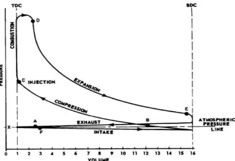
In this section, the principle of the four stroke compression ignition engine is briefly presented. Figures 1.5to 1.7 show the different phases of a classical four stroke Diesel engine cycle. In particular, figure1.5represents the physical phenomena associated with each stroke, figure1.6shows the angular extents of the different phases of the four stroke engine cycle and figure 1.7 represents on the pressure/volume (p−V) thermodynamic diagram the evolutions of the thermodynamic conditions within the cylinder, during a complete engine cycle. In the following, the different Diesel engine cycle phases are discussed more in detail.

Stroke n° 1 : intake

The piston is moving from Top Dead Center (T DC) towards Bottom Dead Center (BDC), figure 1.5. In this first phase, the intake valves are opened and allow the fresh ambient air mixture, composed in the most general case of pure air and Exhaust Gas

Figure 1.5: The Diesel four-stroke operating cycle.

Figure 1.6: Angular extents of the engine cycle phases for a Diesel four-stroke engine.

Recirculation (EGR) gases, to fill the combustion chamber. As the Intake Valve Open- ing/Closing (IV O/IV C) times are finite, in order to optimize the volumetric efficiency, the intake valve opening interval begins before TDC and ends after BDC, figure1.6. The intake phase on the pressure/volume thermodynamic diagram, figure1.7, corresponds to the evolution −−→

AB which, because of the pressure drop of the gases crossing the intake valve seats, lies at a pressure level lower than the atmospheric pressure².

Stroke n° 2 : compression

The piston is moving from BDC towards TDC, figure 1.5. In this second phase, the cylinder is filled with fresh ambient-air gases, the intake and exhaust valves are closed, and the piston compresses the gases within the combustion chamber. The compression

2The pressure/volume thermodynamic diagram shown in figure1.7 refers to a naturally aspirated Diesel engine.

Figure 1.7: Pressure-volume thermodynamic diagram for a Diesel four-stroke operating cycle.

phase begins after BDC and ends at TDC, figure1.6. During this phase, the ambient-air gases heat up and exchange heat with the cylinder walls. Consequently, the compression phase on the pressure/volume thermodynamic diagram, figure 1.7, is represented as a polytropic evolution, −−→

BC. Usually, the liquid fuel injection within the cylinder starts just before the piston reaches TDC. In fact, at this time, the thermodynamic conditions of the gases within the combustion chamber favor the liquid fuel evaporation and the formation of radicals which permits the auto-ignition of the reactive mixture (mixture of fuel and ambient-air).

Stroke n° 3 : expansion

The piston is moving from TDC towards BDC, figure 1.5. In this third phase, both the intake and exhaust valves are closed, and the reactive mixture burns and expands within the combustion chamber. The expansion phase is the major work contribution to the engine cycle. The expansion phase begins at TDC and ends before BDC, figure 1.6.

On the pressure/volume thermodynamic diagram, figure 1.7, the expansion phase is represented by−−−→

CDE. In the evolution indicated as−−→

CD, representing the reactive mixture combustion, two combustion regimes can be distinguished. The first starting around TDC, pointCin figure1.7, and taking place at a constant volume, which corresponds to the auto-ignition of the reactive mixture; the second going up to point D in figure 1.7, which corresponds to the combustion of fuel burning as a diffusion flame³. Then, during the evolution indicated as−−→

DE, the burned gases expand within the cylinder and, at the

3In a diffusion flame the fuel consumption rate is limited by the mixing process between gaseous fuel and oxidizer [91].

same time, exchange heat with the cylinder walls (heat loss). In figure1.7the expansion phase is represented as a polytropic evolution.

Stroke n° 4 : exhaust

The piston is moving from BDC towards TDC, figure 1.5. In this fourth phase, the exhaust valves are opened and the piston movement pushes out the burned gases from the cylinder. As the Exhaust Valve Opening/Closing (EV O/EV C) times are finite, in order to optimize the engine efficiency, the exhaust valve opening interval begins before BDC and ends after TDC, figure 1.6. The intake phase on the pressure/volume thermodynamic diagram, figure1.7, corresponds to the evolution−−→

EF which, because of the pressure drop of the gases crossing the exhaust valve seats, lies at a pressure level higher than the atmospheric pressure.

Diesel operating cycle analysis

Figure 1.8 shows the operation of a typical naturally aspirated Compression Ignition (CI) engine [6]. The represented Diesel engine has a compression ratio, defined as the ratio between the maximum and the minimum cylinder volumes equal to16⁴. The figure shows four plots; in the following the different plots will be indicated using the letters from (a) to (d) as going from the top to the bottom of the figure.

Figure 1.8: Sequence of events during compression, combustion, and expansion processes of a naturally aspirated compression-ignition engine operating cycle [6]. Cylinder volume/dead volume (V /Vd), liquid fuel injection rate (m˙F_l), in-cylinder pressure (p) (solid line, firing cycle;

dashed line, motored cycle), and Heat Release Rate (HRR) are plotted against crank angle.

4Classical values of Diesel engine compression ratios vary between 12 to 24, depending on the type of engine and whether the engine is naturally aspirated or turbo-charged.

Figure1.8(a) shows the evolution of the cylinder volume,V, normalized with respect to the dead volume, Vd, as a function of the crank angle. In figure 1.8 (b), the profile of the liquid fuel injection rate is shown, m˙Fl; the Start Of Injection (SOI) and the End Of Injection (EOI) crank angle values are put in evidence. As seen, the fuel is injected about 20 CAD before TDC. The liquid fuel atomizes, evaporates and mixes with ambient air. After a short delay, the gaseous mixture of fuel and ambient air auto- ignites. The auto-ignition represents the Start Of Combustion (SOC), figure 1.8 (c).

Hence, the cylinder pressure (solid line in figure1.8 (c)) rises above the motored engine level (dashed line). At the SOC, part of the injected fuel which has already mixed with sufficient air to burn, reacts very fast, figure1.8(d). As the expansion process proceeds, mixing between fuel and ambient air continues, accompanied by further combustion in which fuel burns in a diffusion flame regime.

1.1.2 The Common Rail system

The Common Rail (CR) system is one of the key devices that have allowed the strong diffusion of Diesel engines all over the world. In particular the CR system allows higher injection pressures⁵, faster switching times and greater adaptability of the injection pat- tern to engine operating conditions. All these characteristics are necessary for making the Diesel engine more efficient, cleaner and more powerful. The major advantage of the CR system is its ability to vary injection pressure and timing over a broad scale. This is made possible by separating the functions of pressure generation and fuel injection.

Figure1.9 shows a typical CR system integrated in a modern engine architecture.

The CR fuel injection system is made from three subsystems :

• the low pressure circuit charged of supplying the fuel to the high pressure circuit,

• the high pressure circuit consisting of the high pressure pump, high pressure accu- mulator (rail) and injectors,

• the electronic control system made from the sensors, control unit and actuators.

All the injectors, one for each cylinder, are fed by the common fuel rail. The injectors are the most important component of the CR system. They incorporate fast-switching solenoid valves by means of which the nozzle is opened and closed. This enables the injection pattern to be individually controlled for each cylinder.

A continuously operating high pressure pump, driven by the engine, produces the desired injection pressure. Pressure is controlled by a pressure limiter positioned on the rail, figure 1.9. As the pressure is stored in the rail, it is largely independent of

5In the next generation of CR injection systems, the injection pressure can rise up to2000bar.

Figure 1.9: Common Rail injection system [100].

the engine speed and injected fuel quantity. The injectors inject fuel directly into the combustion chamber. The fuel injection is controlled by the Electronic Control Unit (ECU), figure 1.9.

Schematics of the injector and injector tip are shown in figure 1.10.

Figure 1.10: Common Rail injector [52].

The main features of the injector are the solenoid, the control needle, the main needle, and the fuel supply and return lines. The enlargement on the top left in figure1.10can be used to describe the operation of the injector. Activation of the solenoid lifts the control

needle, opening orifice A directly above the main needle. This action allows fuel flow from the supply line through orifice B into the small chamber above the main needle, then through orificeAto the return line. Since orificeB is smaller thanA, the pressure in the small chamber is much less than the fuel line pressure, creating a force imbalance that unseats the main needle and starts the injection. When the solenoid is deactivated a closure spring reseats the control needle. The pressure in the chamber above the control needle then returns to the fuel supply pressure causing the main needle to reseat, ending the injection.

1.1.2.1 The multiple injection strategies

Multiple injection strategies, that is the introduction in the cylinder of liquid fuel mass split into several injections, have permitted a strong improvement in the combustion process in Diesel engines, in terms of performance and pollutant emissions.

Figure1.11shows a double injection pattern : on the top of the figure, is represented the injection command, while on the bottom is represented the corresponding injection rate. The engine operating conditions as well as the injection parameters are given in table 1.1.

Injection1 Injection2

Injected liquid fuel mass [mg] 5 15 Injection advance [CAD BTDC] 35 55

Engine speed [rpm] 3000

Injector opening delay [µs] 350

Injection pressure [bar] 800

Table 1.1: Engine operating conditions and injection pattern variables. The values given in the table refer to the injection pattern shown in figure1.11.

As shown in figure1.11(top), the variables commonly used for defining the injection command of the i^th fuel injection are :

• the Injection Advance (AV I_i), defining the crank angle at which the injection command starts,

• the Energizing Time (ET_i), giving the length of time of the injection command and

• the Dwell Time, (DTi−(i+1)), giving the time interval between the end of the i^th injection command and the start of the (i+ 1)^th injection command.

Looking at figure 1.11 (bottom), it is interesting to note that, for the i^th injection, the AV Ii does not correspond to the Start of Injection (SOIi) of the liquid fuel. This is due

−400 −30 −20 −10 0 10 20 0.2

0.4 0.6 0.8 1

Crank angle [CAD ATDC]

Injection command [−]

Inj1 Inj2

−400 −30 −20 −10 0 10 20

0.01 0.02 0.03 0.04 0.05 0.06

Crank angle [CAD ATDC]

Fuel injection rate [kg/s]

Inj1 Inj2

AVI₁

SOI1

ET1 ET

DT 2 1−2

AVI1 AVI

2

AVI2

SOI₂

Figure 1.11: Multiple injection pattern. The values of the variables defining the injection pattern shown in the figure are given in table1.1.

to the injector opening delay, associated with hydraulic and mechanical inertias, which depends on the injection system.

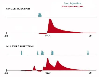
Figure 1.12 schematically represents the difference between single and multiple in- jection strategies in terms of fuel injection rates and Heat Release Rates. As shown in

Figure 1.12: Comparison of the fuel injection rates and Heat Release Rates associated with single and multiple injection strategies.

figure 1.12, the injection strategy pattern strongly influences the Heat Release Rate of

the engine cycle.

The injection pattern shown in figure 1.12contains five injections⁶ (from the left to the right) :

• pilot injection : usually performed very early respect to theSOI of the main injec- tion, it reduces the combustion noise during cold-start and idle regimes. Moreover it contributes to the reduction of soot emissions, and increases the engine volumet- ric efficiency⁷,

• pre injection : usually performed very close to the main injection, it controls the premixed combustion process which has a strong impact on the combustion noise, and on soot and NOxformation,

• main injection : it involves most of the injected fuel mass (70÷80%). Its role is to generate the performance in terms of torque/power demanded by the driver. The SOI associated to the main injection has strong effects on the NO_x formation,

• after injection: usually performed very close to the main injection, it has an impact on the end of the combustion and favors the completion of the soot oxidation process for mainly two reasons :

– it increases the gaseous mixture temperature favoring the oxidation reactions, – the kinetic energy associated to the injected mass of fuel generates turbulence in the cylinder, that favors mixing motion increasing oxygen concentration where necessary for soot oxidation,

• post injection : usually performed very late in the engine cycle, it considerably increases the exhaust gas temperature. Generally, the post injection is adopted in injection strategies performed periodically for improving the aftertreatment device performance :

– quick warm-up of the catalyst,

– regeneration of the Diesel Particulate Filter (DP F), – improvement of lean-NO_x trap efficiency.

6Up to present, the injection strategies adopted for commercial vehicles, never exceed five injections per cycle.

7This effect, commonly observed in gasoline engines, can be encountered in Diesel engines when very early injections are performed in order to obtain homogeneous mixtures burning in HCCI combustion regime. The evaporation of the liquid fuel cools the gaseous mixture in the cylinder. The intake pressure being imposed, a temperature decrease implies a volume decrease and consequently the possibility of introducing more fresh air.

1.1.3 The combustion process

In the last decades, in order to reduce the engine pollutant emissions, many efforts were made in the research domain for understanding the pollutant species formation mechanisms.

It was found that a promising way for reducing the pollutant emissions consists in acting directly on the combustion process.

In fact, the pollutant species formation is strongly related to the local thermochem- ical properties of the mixture within the cylinder. Accordingly, establishing the right in-cylinder thermochemical conditions would allow a reduction of pollutant emissions.

These studies brought to the introduction of non-conventional combustion regimes, such as Premixed Controlled Compression Ignition (P CCI), Low Temperature Combustion (LT C) and HCCI combustion processes, figure 1.13.

Figure 1.13: PCCI, LTC and HCCI concept on aΦ−T map [62].

As shown in figure1.13, the tendency is to obtain a combustion process characterized by lower temperatures and a higher level of local air-excess ratio, in order to get out of the region relative to NO_x and soot emissions. Nowadays, to reduce the combustion temperatures, it is usual to dilute the fuel-air mixture with EGR because of its high specific heat-capacity and immediate availability.

In the following, in order to put in evidence the major differences between con- ventional and non conventional combustion processes, attention will be focused on the differences between conventional Diesel and Diesel HCCI combustions.

Conventional Diesel and HCCI combustion modes are governed by different physical mechanisms.

In conventional Diesel combustion, the mixture inside the cylinder is characterized by a high fuel mass fraction stratification. The first site of auto-ignition appears inside the spray, where chemical and thermodynamic conditions are the most favourable. Heat

released by combustion at the first site, subsequently favors the multiplication of auto- ignition sites. This chain reaction leads to the sharp heat release process typical of the premixed Diesel combustion phase. The remaining fuel burns in a diffusion flame and the heat release is governed by the mixing process. In this phase, turbulence plays the most important role. The dynamics of a convention Diesel combustion are shown in figure1.14.

In figure1.14are clearly distinguished the six injection cones coming out of the injector

Figure 1.14: Dynamics of a conventional Diesel combustion [100].

nozzle, which is positioned at the center of the combustion chamber. The injected fuel penetrates within the cylinder and mixes with ambient-air. As seen, the gaseous mixture within the cylinder is strongly heterogeneous, hence, the local thermochemical properties of the gases strongly vary in terms of temperature and equivalence ratio. In the conventional Diesel regime, combustion is essentially controlled by mixing.

On the other hand, in HCCI combustion, the mixture inside the cylinder is homoge- neous. Hence, chemical kinetics play the most important role in the combustion process.

The dynamics of a Diesel HCCI combustion are shown in figure1.15.

As shown in this figure, because of the homogeneity of the mixture, all the gas auto- ignites simultaneously. As a consequence, HCCI combustion is characterized by a high Heat Release Rate (HRR).

1.2 The global engine system study

An ICE is a complex system to study for the following reasons :

• many different branches of physics are involved in the study of its fundamental principles of functioning,

-11.4 CAD ATDC -10.8 CAD ATDC -10.2 CAD ATDC -9.6 CAD ATDC

-9.0 CAD ATDC -8.4 CAD ATDC -7.8 CAD ATDC -7.2 CAD ATDC

Figure 1.15: Dynamics of a Diesel HCCI combustion [98].

• complex interactions between physical phenomena occur,

• the large number of devices integrated in the engine architecture, which are nec- essary in order to guarantee the required flexibility to the system, constitute a complex system to optimize,

• prototypes are expensive to manufacture and need time to be tested.

For these reasons, the optimisation of the entire engine system is a hard task, expensive and time consuming. In the following, two devices for optimizing the performance of global engine systems are presented :

• experimental global engine test bench,

• global engine simulation numerical models.

1.2.1 The global engine system test bench

In the past, the global engine test-bench was widely used for engine-control calibration, figure1.16. This methodology of calibration was possible essentially because :

• only a reduced number of devices were integrated in the engine architecture,

• the engine systems were less flexible,

• there were less constraints in terms of pollutant emissions,

• it was the only solution available then.

The major inconvenients associated to this methodology are :

• the cost in terms of facilities and human resources,

• the length of time needed for the experiments.

Today, the role of the engine test-bench in the engine development process has changed.

In fact, it is essentially used for :

• testing very particular engine operating points,

• testing new engine control strategies,

• validating the ICE numerical simulations,

and no longer used for optimizing engine control strategies.

Figure 1.16: Schematic of a global-engine test-bench.

1.2.2 The global engine system simulation

In recent years, consequently to the rapid progress in CPU performance and the large increase in data storage capabilities, numerous softwares for global engine system numer- ical simulation have been developed (e.g. GT-power, AMESim, GASDYN, etc...). As mainframe for the development of dual-CM, the environment of simulation AMESim has been choosen, appendix A. Compared to global engine test bench approach, the global engine system simulation presents the following advantages, figure 1.17:

• the cost in term of facilities and human resources is relatively low,

• computations are performed in a short interval of time,

• the models can be easily transported from one place to another.

On the other hand, global engine system simulation is not a stand alone device : it needs experimental data from laboratory facilities in order to validate the engine model. In industry, global engine system simulation is mainly used in the following domains :

• engine architecture conception phase,

• engine-control strategies definition,

• engine performance investigation, (e.g. engine tests on standard vehicle homolo- gation driving cycles).

Figure 1.17: Schematic of a global-engine system simulator.

1.3 Objective and methodology

The aim of this work is to develop a numerical model able to simulate the ICE com- bustion process in both conventional Diesel and Diesel HCCI regimes. The model has been conceived for global system simulation applications. In this context, the model must be able to respond properly to turbocharger pressure variations, which modify the thermodynamic conditions of the inlet gases in the cylinder in term of pressure and tem- perature, fuel injection pattern variations, Exhaust Gas Recirlculation (EGR) mass flow rate variations, etc...

The development of such models is a challenge especially because :

• the large number of physical fields that occur in ICEs (multidisciplinary compe- tences),

• the complex interaction between the different physical phenomena during the com- bustion process,

• the large magnitude ranges on spatial and temporal scales associated to the phe- nomena that must be modeled and taken into account,

• the wide range of engine conditions constituting the engine operating domain,

• the fact that global system simulation tools are limited to 0D approaches requires more modeling and parametrization than classical 3D CFD.

In the following, the dissertation focuses on the study and comprehension of the combus- tion process in Diesel HCCI engines, that is engines that are able to run using conven- tional Diesel and Diesel HCCI combustion regimes. In chapter 2, the developed model, dual Combustion Model (dual-CM), is introduced and detailed. The different submodels constituting dual-CM have been developed and validated on the base of the observations made by using experimental facilities : both published in literature or coming from the IFP laboratories. When experiments were not available, submodel validations were done on the basis of computed results obtained by using numerical solvers considered to pro- vide reliable physical results. In chapter3, the engine validation results of the dual-CM are presented. The model has been validated using engine test bench experimental re- sults when available and 3D CFD simulation results when experimental data were not available. In chapter 4, the limits of the model are investigated and precision analysis are carried out.

The dual Combustion Model (dual-CM)

In this chapter the dual Combustion Model (dual-CM) is presented. Dual-CM has been conceived following the outline of the promising approach developed by Mauviot [13] at IFP.

During this Ph.D, the original model of Mauviot [13] was improved following three major axis of development :

• introducing new features in order to extend the application domain of the combus- tion model. This aspect essentially concerns the introduction of a new formalism able to take into account multiple injection strategies : from the description of the evolutions and interactions of the different sprays within the cylinder, up to the description of the complex chemical kinetics,

• introducing more physics in the different submodels, in order to make the combus- tion model more predictive. In particular :

– a description of the liquid-gas interface during the evaporation process was introduced. This aspect is very important in the determination of the local thermochemical properties of the gaseous mixture and, consequently, on the determination of the mixture auto-ignition delay,

– a new equation for the fuel mixture fraction variance was developed. The new formula takes into account the fact that liquid fuel evaporates in ambient-air at saturated conditions and not as a pure fuel. Moreover, the new equation is adapted to be used in a multiple-injection context, in which the spray associated with the different fuel injections can interact with one another, – a new formulation of the chemical kinetic model, permitting us to have a

better description of the species evolutions during the combustion process and a better estimation of the final composition of the exhaust gases was adopted.

In particular, the new chemical kinetic model is based on a species mass fraction complex chemistry tabulation method instead of a species reaction rate complex chemistry tabulation method,

– the chemical kinetics mechanism used for generating the table is the one proposed by Anderlohr [86] for n-heptane. This mechanism, compared to the

31

one used in the original version of the model [64], permits to have a better estimate of the mixture auto-ignition delays,

• optimizing the source code in order to reduce to the bare minimum the computa- tional time, compatibly with the modeling solutions that were retained.

All these aspects will be discussed in detail in the following of this chapter.

First of all the context and the specifications of dual-CM are introduced, section 2.1.

After that, starting from the state of the art in combustion science applied to modern Diesel HCCI ICE, section 1.1, several physical topics are retained and considered as fundamental for the description of the in-cylinder combustion process and consequently studied, interpreted, modeled and integrated in dual-CM. Essentially, the physical topics retained and presented in section2.3to 2.6are the following :

• liquid fuel injection,

• composition evolution,

• turbulence,

• chemical reactions,

• thermal exchange losses,

• combustion chamber geometry variations,

• fluid thermodynamics.

A parametric study of dual-CM, section 2.7, shows the sensitivity of the model to the different modeling parameters. Finally, the dual-CM computational time is discussed, section2.8.

2.1 Context and model specifications

The dual-CM is a 0D phenomenological combustion model formulated for global engine system simulation, subsection1.1, and especially for Diesel HCCI engines, section1.2.2.

In this sense, the model must be able to provide reliable results in short computational time. The model has been conceived by reducing physical 3D CFD models to a 0D formalism. The different submodels constituting dual-CM have been developed by using as much as possible physical information and reducing to the bare minimum the use of abstract empirical/mathematical laws. This choice is a scientific challenge because reducing the number of pure modeling adjustment coefficients, reduces the possibility to tune computed results in order to fit experimental data. On the other hand, it brings the following advantages :

• using the model is intuitive because adjustment parameters are associated with physical phenomena,

• computed variables can be interpreted as representative of the real physical process and, consequently, used to study trends and limiting factors of the real system,

• once the model is tuned to a given set of engine operating points, it is expected to be able to predict the behavior of the system for different operating conditions, too,

• the model can be used in the engine architecture design process,

• the model can be used in engine-control strategy definition in which predictivity is a fundamental need.

The aim of the model is to be able to predict the in-cylinder combustion process once :

• devices such as turbochargers, EGR system, intercoolers, wastegate valve, Variable Valve Actuators (VVA) have imposed in the cylinder a mixture of air and eventually EGR at given thermodynamic conditions,

• a fuel injection strategy pattern has been defined.

Essentially, during the Ph.D, modeling efforts have focused on :

• liquid fuel evaporation,

• reactive gaseous mixture zones (spray regions),

• Auto-Ignition (AI) delays of reactive mixtures,

• Heat Release (HR),

• major pollutant species chemical-kinetics,

• Indicated Mean Effective Pressure (IMEP).

A model being able to satisfy all these requirements is suitable for the integration in a global engine system simulator. In fact, such a model is able to fully interact with the other devices integrated in the engine architecture : responding to the different system inputs and providing the necessary outputs to the system. In the following, the presentation will focus on the modeling of compression and expansion strokes of the Diesel thermodynamic cycle, which are the only phases of the engine cycle concerned with the combustion model.

2.2 Synoptical diagram of the model

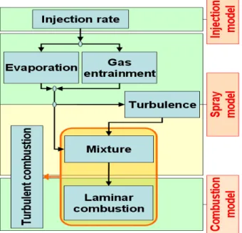
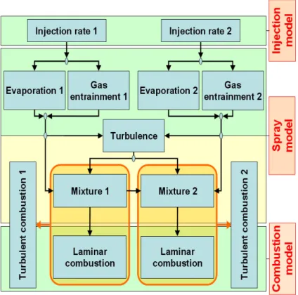
In dual-CM the different physical phenomena, taking place in the cylinder of a Diesel HCCI engine, are taken into account and described by proper submodels, figure2.1. In

Figure 2.1: Synoptical diagram of the model dual-CM in a case of single injection strategy.

the following, the investigation will focus on the interval of the engine thermodynamic cycle going from Inlet Valve Closure (IVC) crank angle, during the compression stroke, to Exhaust Valve Opening (EVO) crank angle, during the expansion stroke, considered as being the only crank angle interval in which combustion conditions occur in the cylinder.

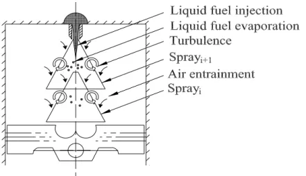
At IVC crank angle, an ambient gaseous mixture, consisting of pure air and eventually EGR, is compressed by the piston. This ambient mixture is here supposed to be a perfectly stirred mixture. As shown in figure 2.1, the event triggering the combustion computation is the injection of liquid fuel in the combustion chamber (Injection rate model, section2.3). At that point liquid fuel and ambient air coexist within the cylinder.

The region where both fuel and ambient-air are simultaneously observed is called spray region (Spray model, section 2.4), figure2.2. Two main phenomena occur in the spray region :

• the liquid fuel evaporation (Evaporation submodel, section2.4.1),

• the entrainment of ambient air in the spray (Gas entrainment submodel, sec- tion2.4.2).

As liquid fuel evaporation and ambient air entrainment go along, the spray region grows.

The injection of liquid fuel at high speed in the cylinder introduces a large quantity of

Figure 2.2: Schematic of the liquid-fuel injection phisics within the cylinder of a Direct Injection Diesel engine.

kinetic energy which is finally transformed in a strong turbulent motion (Turbulence sub- model, section2.4.3). The presence of turbulence in the combustion chamber favors the mixing between gaseous fuel and ambient gas. Consequently, a continuous distribution of mixture compositions varying from a maximum fuel mixture fraction (correspond- ing to ambient-air saturated with fuel, Z = Z_s¹) to pure ambient-air (corresponding to Z = 0) is present in the cylinder, section 2.4.4. Because of the turbulent mixing process, the mixture inside the cylinder tends to become progressively more homoge- neous. Among the wide spectrum of mixture compositions within the cylinder, the compositions contained between the fuel inflammability limits are named reactive mix- tures. Once favorable thermodynamic conditions are reached, the combustion process takes place (Combustion model, section2.5). Focusing on a given composition belonging to the reactive mixtures, the oxidation process takes place once the auto-ignition delay is reached. At that instant, combustion begins. During the combustion process, thou- sands of intermediate chemical species appear and interact with one another eventually forming products of combustion and pollutant species (Laminar combustion submodel, section2.5.1). In a Diesel HCCI combustion chamber, mixture is not homogeneous and local composition varies in time because of the turbulence action (turbulent mixing).

Those are very important aspects to be accounted for in Diesel HCCI combustion and they influence the whole combustion process from the auto-ignition delay to final mixture composition (Turbulent combustion submodel, section 2.5.3). Until now, the discussion has been limited to single injection strategy configurations. Things change slightly for multiple injection strategy configurations. A diagram representing a multiple injection strategy configuration is shown in figure 2.3 for double injection strategies. Obviously, before the start of the second injection, the diagram of the model is identical to that

1Definition and modeling ofZsare discussed in detail in section2.4.1.1.

Figure 2.3: Synoptical diagram of the model dual-CM in a case of multiple injection strategy.

of the single injection case. When the second injection starts, the diagram is modified because the two injections interact : the impact of the second injection on the first one can be summarized as an enhancement of its kinetic energy. On the other hand, the impact of the first injection on the second one is much more important :

• the velocity field within the cylinder has been modified by the first injection,

• the thermodynamic conditions within the cylinder have been modified by the com- bustion of the fuel of the first injection,

• the entrained air in the spray region of the second injection has a chemical com- position that is different from that of the ambient air, as it has been modified by the combustion of the fuel of the first injection,

• the chemical kinetics of the mixture formed by the second injection is influenced by both the different chemical composition and the different thermodynamic con- ditions of the entrained ambient-air.

Certainly, other effects associated to the interaction of different sprays exist. In a first approximation, all these are neglected.

2.3 Injection rate model

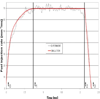
The fuel injection rate model is fundamental in order to perform an engine cycle com- putation. It simulates the response of the high pressure injection system to the inputs received from the Engine Control Unit (ECU). In particular, it computes the liquid-fuel mass introduction rate, m˙_Fl, in the cylinder. As can be seen in figures 2.1 and 2.3, it is the main input of the dual-CM spray model, section 2.4, and in particular it directly communicates with the evaporation submodel, section 2.4.1, and the gas entrainment submodel, section 2.4. In order to correctly characterize an injection rate profile (fuel flow rate versus time), the aspects that must be accounted for are, figure 2.4:

• the initial slope, describing the opening transitory of the injector needle (the needle opening transitory is mainly due to the unbalanced fluid pressures acting on the needle and the needle inertia),

• the maximum value of the injection rate, corresponding to a steady opening state,

• the final slope, describing the closing transitory of the injector needle (the needle closing transitory is mainly due to a mechanical force acting on the needle),

• the integration of the fuel injection rate curve must be equal to the injected fuel mass.

All these aspects vary with the technological parameters of the injection system :

• the injection pressure,p_inj,

• the energizing time,ET,

• the nozzle permeability,

• the injector geometry,

• the type of fuel.

In order to account for all these aspects, an injector model has been developed at IFP.

For a given fuel, injector and nozzle, the model is able to describe the fuel injection rate as function of the time. Moreover, the model is sensitive to injection pressure and energizing time variations. In this approach, an injection rate profile relative to high injection pressure (here p^ref_inj = 1600 bar) and sufficiently long energizing time² (here ET^ref = 2.25 ms) is chosen as reference injection profile, figure 2.4. Figure 2.4 shows the main features of a reference fuel introduction rate profile. In particular, the three different regions characterizing the injection profile can be clearly distinguished :

2A correct energizing time value must guarantee the complete lifting of the injector needle.

Figure 2.4: Description of the main features of a reference fuel introduction rate profile.

the initial transitory (left), the steady condition (middle) and the final transitory (right).

The first step, in order to have an analitical expression of the reference liquid fuel injection rate,m˙^ref_F

l , consists in fitting the experimental reference injection rate with appropriate equations, in each region :

• the opening period (fromt^ref₀ tot^ref₁ ) is modeled by using a sixth order polynomial :

˙ m^ref_F

l =a₀+a₁·t+a₂·t²+a₃·t³+a₄·t⁴+a₅·t⁵+a₆·t⁶ (2.1)

• the steady injection rate time (fromt^ref₁ tot^ref₂ ) is modeled by using a zeroth order polynomial (constant value) :

˙ m^ref_F

l = ˙m^st_F

l (2.2)

• the closing period (fromt^ref₂ to t^ref₃ ) is modeled by using a first order polynomial :

˙ m^ref_F

l = ˙m^st_Fl−b0·(t−t^ref₂ ) (2.3) experiments showed that the closing transitory slope is independent of the injection pressure,

where a0, a1, a2, a3, a4, a5, a6 and b0 are adjustment coefficients depending on the injection system,m˙^st_Flrepresents the mean experimental injection rate on the time interval t^ref₁ ≤t < t^ref₂ , andt^ref₂ corresponds to the beginning of the closing transitory.

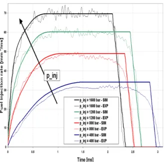
These polynomial expressions are then parametrized with the injection pressure, in order to obtain injection rate profiles for different injection conditions :