%0$503"5%&-6/7&345² -6/7&345²%&506-064& %&506-064&

(1)

%NVUEDELOBTENTIONDU

%0$503"5%&

%0$503"5%&-6/7&345² -6/7&345²%&506-064& %&506-064&

$ÏLIVRÏPAR $ISCIPLINEOUSPÏCIALITÏ

0RÏSENTÏEETSOUTENUEPAR

4ITRE

*529

%COLEDOCTORALE 5NITÏDERECHERCHE

$IRECTEURS DE4HÒSE

2APPORTEURS LE

Institut National Polytechnique de Toulouse (INP Toulouse)

Mécanique, Energétique, Génie civil et Procédés (MEGeP)

Analysis and control of self-sustained instabilities in a cavity using reduced order modelling

Analyse et contrôle des instabilités dans une cavité par modélisation d’ordre réduit

lundi 8 février 2010

Kaushik Kumar NAGARAJAN

Dynamique des fluides

Jean-Pierre RAYMOND, Professeur, Université Paul Sabatier, IMT, Toulouse, Président Christophe AIRIAU, Professeur, Université Paul Sabatier, Toulouse, Directeur Laurent CORDIER, Chargé de recherche CNRS, LEA/CEAT, Poitiers, Examinateur

Angelo IOLLO, Professeur, Université Bordeaux, IMB, Bordeaux, Rapporteur Bernd. R NOACK, Directeur de Recherche CNRS, LEA/CEAT, Poitiers, Rapporteur

Christophe AIRIAU, Professeur, Université Paul Sabatier, Toulouse Azeddine KOURTA, Professeur, Polytech Orléans, PRISME, Orléans

Institut de Mécanique des Fluides de Toulouse (IMFT)

(2)

Acknowledgments

Thomas Alva Edison once said: ”100% Success = 99% perspiration + 1% inspiration” ! for me, the ratio of perspiration to inspiration didn’t trigger my thoughts as much as the truth that inspiration is more dense, deeper and carries equal weight! Without being ‘calculative’ in expressing myself, I would still have to admit my anxiety of making understatements:

I cannot thank enough my supervisors Christophe Airiau and Azeddine Kourta who have moti- vated me to stretch my forte and my competence beyond limits and thereby helped me discover my inner strength which I was not aware of. I owe the success of my efforts and the brightness of my future to them. Christophe brought to this work the insight and rigor in many parts especially concerning ‘Control’. I am very indebted to him for having instilled in me a sense of rigor in my research, as well as in presenting this work. His concern to make his students learn the state-of-art was very well ref ected in the many workshops I attended during the three years.

Words fail to express my gratitude to Laurent Cordier from LEA Poitiers, who has for the most part of the work served as a virtual supervisor. His knowledge in POD based Reduced Order Modelling was indispensible. His rigor and never-say-die attitude has rubbed off on me for life. He has held the guiding light for me to tread this path and has encouraged me all-through. His guidance and constructive criticism have been like stepping stones in the process. Thanks for his great patience in talking to me practically everyday and advising me. Apart from this, I enjoyed the moments of long discussions I had with him on almost every topic.

I sincerely thank Bernd Noack and Angelo Iollo for accepting to be a part of the jury. Their deep knowledge of the state-of-art was ref ected in the many questions they posed and has encouraged me to pursue this f eld further in my career. I would also like to thank Jean-Pierre Raymond for agreeing to preside over the defence presentation. I would also like to remember him for the good lunches I had at his home, his lively spirit and love for Mathematics. I would also like to acknowledge Professor Pierre Comte of LEA Poitiers for providing me with a copy of his DNS code and his help during the initial days of the work.

Thanks for the support I received from the Service Informatiques during the last three years.

Special thanks to Nicolas Renon of CICT for providing me various tips on large-scale computation.

Thanks to Marie Christiani secretory of the group for coordinating the various activities of the project.

Her enthusiasm to help foreign students in many day-to-day activities is noteworthy. I would also like to thank V´eronique Cassin, the new secretory, for her help during the last days of the work.

Special thanks to the various partners of the AeroTraNet project who gave a new direction on solving a problem by combining the various aspects of work like numerical, experimental. The bi- annual meetings gave me an unique opportunity to network with various researchers working on different aspects of the same problem. I would also like to thank peers in the f eld whom I met during many conferences and workshops. Thanks to Clancy Rowley, Dietmar Rempfer, Ravindran for providing many exciting perspectives of thought. A special acknowledgment goes to John Burkardt from Florida State University for maintaining the best collection of libraries of various programs which have been used in this work. I have copied his style of programming!

Thanks to Laia and Sivam, mes amies in this long sejour of three years, who have stood by me and encouraged all along. Laia has been a great support till the last days of my thesis. Her

(3)

uncanny ability to organise things leaves me awe-struck. Sivam by sharing his treasure of Tamil songs made my days lively. Thanks to my other friends Karim, Anais, Houssam, Remi, Wafa, Marguerite, Thibaud, Benjamin, Romain, Xavier, Rudy, Mariyana, Bernard, Dirk, Yannick, Marie, Omar, Luigi, Sheetal and Aalap for their support and encouragement. I would like to acknowledge Yogesh for suggesting many improvements in the write-up. Thanks to David for giving me various tips for my f nal presentation.

I owe my heart f lled thanks to my parents; especially my mother (Smt. Girija Nagarajan), brother and sister-in-law (Ishwar & Ramya), sisters - Rani, Preethi, Gowri (Chinni included) for their encour- agements, forbearance, support and prayers and having stood by me during ‘high and low tides’, for the unfaltering faith they had in me, which was an essential base to the victorious atmosphere I’m breathing in, right now.

Thanks to my friends the Badri-boys (Dilip, Guru, JP, Kiran, Parag, Sriram, Sreenidhi, Vivek), Di- vya and Swathi for their constant encouragement and prayers for my betterment. I would like to thank Raghoothamachar for cultivating in me a sense of unbiasedness while pursuing knowledge. Thanks to Dr. Ramesh (NAL) for encouraging me in my pursuits. I would also like to thank Dr Kirti Malhotra and Dr N. Balasubramanya my undergraduate professors. Thanks to Professor A.S.Vasudevamurthy of TIFR for his words of motivation to come abroad for a PhD.

There is no greater blessing than to have the guidance of an enlightened personality. All our knowledge, inspiration and wisdom are dormant within us as seeds. The proper watering through spiritual guidance nurtures these seeds to grow into deep-rooted, majestic trees. That kind of initiation is what I have received from Shrila Prabhupada. This seed was further cultivated and enriched by Shri Bannanje Govindacharya by showing me a new light, leading to the path of Shri Madhwacharya, who is immanent in every soul, the preceptor of all the worlds and the embodiment of all virtues.

Last but not the least, all these thanks-giving would have no real meaning if I fail to recognise the Supreme Lord Shri Krishna, immanent in all of them. I humbly dedicate this work unto His lotus feet with heart-felt prayers. I would like to admit that I too am a mere instrument in this progression.

This thesis has been supported by a Marie Curie Early Stage Research Training Fellowship of the European Community’s Sixth Framework Programme under contract number MEST CT 2005 020301.

(4)

Annexes 141

A Controllability and observability of linear systems 141 B Galerkin projections for the full NS equations 143 C Specif c volume formulations of ROM 145 D Actuated POD by the method of stochastic estimation 147 E Theorem concerning actuated mode 149 F Generalized Singular Value Decomposition (GSVD) 153 G Open loop control 155 G.1 Open loop control of cavity f ows. . . 155

G.2 Resolving the optimal system . . . 156

G.3 Open loop control of cavity . . . 158 H An open loop approach to handle the acoustic terms in ROM 161

(7)

References 163

(8)

General Introduction

Motivation

Les émissions acoustiques représentent un des problèmes majeures du transport aérien qui concer- nent l’environnement. Généralement on classe les bruits émis en fonction de leur origine mécanique, aérodynamique et ceux liésaux systèmes secondaires. On s’intéresse ici au bruit émis au voisi- nage des aéroports, et il provient pour l’essentiel (voir figures 1 et 2) de l’écoulement autour du train d’atterrissage, de celui des jets de réacteurs et de différentes cavités présentes sur l’avion.

Nous allons dans la suite considéré uniquement la géométrie de la cavité dont l’écoulement est schématiquement donné sur la figure 3 et 4, en fonction du rapport d’aspect. Le travail présenté ici consiste à analyser la physique de l’écoulement et de la propagation du bruit et surtout à chercher

à réduire les émissions acoustiques.

Différents approches expérimentales par un contrôle passif ou actif de l’écoulement ont pu déjà être testées avec plus ou moins de succès, grâce en particulier aux avancées techniques dans les moyens de mesures et de de contrôle, et dans le domaine des ressources informatiques. Actuellement, en utilisant les Simulations Numériques Directes (DNS) ou les Simulations à Grandes Echelles (LES) nous sommes en mesure de mieux comprendre la physique de cet écoulement. Par contre, compte tenu de l’énorme dimension du problème, les études numériques et théoriques du contrôle acoustique doivent nécessairement passer par la réduction de modèle (ROM, voir figure5). Ici nous appliquerons la Décomposition en Valeurs Propres Orthogonales (POD), qui permettent finalement de réduire la complexicité des équations de Navier-Stokes à la résolution et donc au contrôle, d’un systèmes d’équations au dérivées ordinaires (ODE, voir figure 6), plus simple à manipuler et résoudre. En se basant sur les travaux précédents de Rowleyet al.(2003), Gloerfelt(2008), Kasnako˘glu(2007), Samimyet al.(2007) et deCordieret al.(2009), nous allons proposer un contrôle du système réduit, une fois celui-ci calibré et l’appliquer ensuite sur le système complet issu des Simulations Numériques Directes.

Ce travail a été effectué dans le cadre d’un projet Marie-Curie appelé AeroTraNet, mené en collaboration avec3universités étrangères. Le LEA de Poitiers a largement contribué aux différentes parties: L. Cordier pour ce qui concerne la réduction de modèle, P. Compte pour les DNS.

(9)

Organisation du document

La chapitre 1 introduit l’outil de simulation numérique de base (DNS). Les éléments de la théorie du contrôle utilisés plus tard sont présentés dans le chapitre 2. Le chapitre suivant est consacré à la réduction de modèle et son application sur l’écoulement de cavité. Le système dynamique obtenu est fortement instable aussi le chapitre 5 est dédié à la calibration et la stabilisation du modèle réduit.

De multiples approches sont abordées. Le contrôle du système dynamique forcé et son effet sur l’écoulement complet, sur la base de la théorie du contrôle linéaire quadratique gaussien sont finale- ment présentés dans le chapitre 5. Une conclusion suivi de quelques annexes achèvent le document.

Motivation

The recent rise in the air travel has given rise to a number of environmental concerns of which an important issue is the noise. Exposure to noise, particularly near the airports have been known to cause a number of health problems, like stress, hearing problems, hypertension, cardio-vascular problems, sleeping disorders. A constant exposure to noise levels beyond65−70dB is known to cause life term health effects.

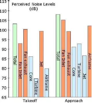
Noise emitted from an aircraft can be broadly classif ed as mechanical noise, aerodynamic noise and aircraft system noise. Mechanical noise is usually caused due to propeller, jet engines. The main source of mechanical noise in an aircraft occurs during cruise conditions, due to the high velocity of jet from the engine. The aerodynamic noise arises due to the airf ow around the different geometric conf gurations such as fuselages, high lift devices devices, landing gears, head and tail rotors of a helicopter etc. Aircraft system noise is mainly due to the cabin pressurisation as well as due to the auxiliary power units used to start the main engines, to provide power during ground conditions.

Although during cruise conditions the mechanical noise dominates, the aerodynamic noise assumes an equal proportion during landing and takeoffs. Most of the aerodynamic noise during landing and take-offs can be associated to the landing gear, the geometry of which can be modelled as a cavity.

Figure 1 shows the various components of noise sources during the landing or takeoff of aircrafts.

Typical values of perceived noise, due to various components, during take off and landing is shown in f gure2.

A similar phenomenon can also be seen in other conf gurations such as weapon bays, joints between high speed train bogies, car body openings. This brings to interest the study of cavity f ows, particularly when in search of quieter aircrafts as envisaged in the report European aeronautics: a vision for 2020 byEC(2001) .

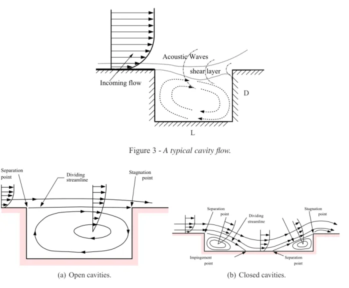
A typical cavity f ow conf guration is as shown in f gure3. The physics of the cavity can be explained by the formation of the shear layer at the upstream cavity edge. As the shear layer propagates it breaks down due to the Kelvin-Helmholtz mechanism resulting in a membrane like oscillation. The shear layer impinges the downstream edge of the cavity and splits, resulting in the formation of vorti- cal structure close to the downstream edge, and is of the size of the depth of the cavity. This results in the formation of acoustic waves which propagates into the upstream, causing the far-f eld noise. The cavity can be classif ed based upon the f ow mechanism it generates, as an open cavity or a closed

(10)

Figure 1 -Typical airframe cavities. (Picture courtesy Ben Pritchard, airliners.com)

Figure 2 -Aircraft noise sources, during approach and takeoffOwens(1979).

cavity. Open cavities are characterised by the shear layer which attaches near the downstream corner, whereas closed cavities are characterised by the shear layer attachment at the bottom of the cavity and separation downstream. The basic difference can be summarised in f gure4. Open cavities are further divided into deep cavities and shallow cavities based on the aspect ratio _D^L. Deep cavities are charecterized by an aspect ratio _D^L < 1, and shallow cavities by aspect ratio _D^L > 1. Many of the airframe structures shown in f gure 1can be treated as a shallow open cavity. The main interest of this work is then to study these f ows and to reduce the noise due to the acoustics.

There has also been numerous attempt to reduce the noise emitted from a cavity, by many heuristic

(11)

shear layer Acoustic Waves Incoming flow

L

D

Figure 3 -A typical cavity flow.

Dividing streamline Separation

point Stagnationpoint

(a) Open cavities.

Stagnation

Impingement Separation

Separation point point

Dividing streamline

point point

(b) Closed cavities.

Figure 4 -Schematic representation of open and closed cavities.

means such as modifying the geometry by means of castellations, spoilers at the upstream edge of the cavity, so as to change the turbulent scales and hence reduce acoustic emissions. Use of synthetic jets delays the re-attachment of the shear layer and has been used in many experiments. With the advent of high performance computing as well as advanced experimental techniques such as the Particle Image Velocimetry (PIV), Laser Doppler Velocimetry (LDV) deep insights into the physics of cavity f ows can be explored, with an aim to reduce the noise.

The traditional approaches like Direct Numerical Simulation (DNS) involve fully resolving the equations governing the f ow dynamicsi.e.the Navier-Stokes’ equations down to the f nest scale. Al- though this approach seems attractive it has inherent diff culties like the computational resources. An approach to reduce the computational time is the utilisation of Large Eddy Simulation (LES) where the major structures governing the f ow (large eddies as they are called) are resolved and the f ner scales are modelled. This approach also poses diff culties, particularly when used as an iterative tool for f ow control, due to their high dimensional nature. The next proposition to reduce the dimen- sionality of the problem is by restricting our interest to the ”most essential structures” which governs

(12)

the dynamics. The basic observation of f uid f ow as a cascading phenomenon gives us the hint of this ”essential” structures in terms of the energy, to obtain a low dimensional space. The reduced order model is then constructed as a projection of the high dimensional dynamics onto this lower dimensional subspace as summarised in f gure5.

Navier-Stokes DNS/LES ROM

Figure 5 -Philosophy of reduced order modelling.

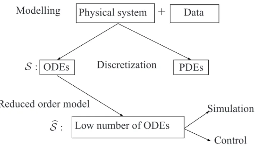
The aim of this thesis is to construct reduced order models for the cavity f ows. The basic idea is to retain the most essential features of the f ow called Proper Orthogonal Decomposition POD modes, which contain the maximum amount of information about the f ow dynamics. By performing a DNS of the compressible Navier-Stokes equations to compute the f ow of a large cavity, the POD modes are extracted. The Reduce Order Model (ROM) is then obtained by projecting the governing equation of f uid f ow i,e the Navier Stokes equations on the subspace spanned the POD modes. This results in one having to solve a system of Ordinary Differential Equations (ODE) rather than the complicated system of Partial Differential Equations (PDE) and hence the name reduced order modelling. The well developed control theory is applied on this system of ODE’s to obtain the noise reduction. Apart from being used in-lieu of the high f delity model for control studies, the reduced order model obtained can also be used as a predictive tool to save computational resources. The overall strategy of using a reduced order model (ROM) can be summarised as shown in the f gure6.

Physical system + Data

S : ODEs Discretization PDEs

Sb: Low number of ODEs

Simulation Control Modelling

Reduced order model

Figure 6 -A Schematic representation of Reduced Order Modelling.

Flow past an open cavity has been studied using ROM byRowleyet al.(2003) andGloerfelt(2008) but without any application to f ow control. More recently, ROM for controlled conf gurations has

(13)

been proposed by Kasnako˘glu(2007). In Samimyet al.(2007) the ROM for f ows issued from an experiment has been used to design a controller. The major hurdle in using the ROM for control applications is the accuracy of the model in predicting the dynamics of the system even for short periods. Also diff culty arises when the control parameters are changed as in a real time simulation.

Various numerical strategies termed as calibration techniques has been developed in the recent past to treat this problem as found inCordieret al.(2009). The major contribution of this thesis is then to complete the full development as applied to cavities, like building up the ROM, including the effect of control, calibrating the model and f nally performing control studies.

The outcome of the interest in reducing the cavity noise has resulted in the frame work of Aero- TraNet (Aerodynamic Training Network) projected which was a collaboration of4academic partners in Europe. The academic partners which included University of Leicester (U.K.), the Universit`a degli Studi Roma Tre (Rome, Italy), Politecnico di Torino (Turin, Italy) and Institut de M´ecanique des Fluides de Toulouse (Toulouse, France) were interested in various aspect of the cavity f ow, like, numerical, experimental and f ow control. This thesis was done in collaboration with LEA Poitiers, P.

Comte for the DNS and L. Cordier for reduced order modelling. The thesis can be summarized as follows.

Organisation of the thesis

In chapter1we give a brief description of the numerical tool, namely the DNS used in this study and present some validation results. In chapter2the basic tools from control theory are introduced.

Chapter3concerns the basic theory of the technique of POD based ROM. The various techniques to include the effect of actuation in the ROM are summarized, with an application to the cavity f ow.

In Chapter 4 the various def nitions of errors between the calibrated dynamics and the original temporal dynamics are introduced and the different methods of calibration summarized are applied to the cavity f ows. The methods are compared for accuracy. The calibration of the ROM is performed using a Tikhonov based regularization to obtain an accurate representation of the dynamics. We also present an improvement of the technique by introducing various type of weight matrix used in the def nition of error. In the f rst method, we use a sensitivity analysis of the ROM, to determine the weights of the relevant terms which needs to be calibrated. The second approach is to use the energy content of the POD representation in forming the weight matrix to represent the errors.

In Chapter 5a feedback control law based on the estimation of the observer dynamics has been presented. The observer matrix is constructed using a linear stochastic estimation. A sensititivity study of the actuated dynamics has been performed to determine the relevant terms in the linearisation of the model. Finally an Linear Quadratic Gaussian (LQG) controller is designed to obtain an optimal solution, which is introduced in the Direct Numerical Simulation to obtain a decrease in spectra of the cavity acoustic mode.

(14)

Chapter 1 Description and validation of the numerical tool

Description et validation de l’outil num´erique

Dans cette partie, les outils numériques utilisés pour les études de modèle réduit et du contrôle sont décrits. Le jet synthétique est introduit pour contrôler les instabilités de cavité. L’écoulement de cavité est largement étudiée dans la littérature. Il présente des instabilités auto-entretenues qui sont difficiles à prédire numériquement (sensibilité aux différents paramètres numériques). La cavité est aussi le siège d’intéractions aéroacoustiques qui nécessitent un schéma numérique d’ordre supérieur et peu dissipatif pour capter les ondes acoustiques. Le code NIGLO utilisé est développé par Pierre Comte de l’Université de Poitiers. Il est capable de résoudre les équations de Navier Stokes com- pressibles en instationnaire et en tridimensionnel. La discrétisation différences finies de quatrième ordre est faite sous forme conservative.

Param`etres de non-dimensionalisation

Le code résout les équations sous forme adimensionnelle. L’adimensionalisation dépend fortement des échelles caractéristiques pour rendre les variables adimensionnelles. La forme adimensionnelle des équations de Navier-Stokes incorpore trois nombres adimensionnel, les nombres de Reynolds, de Mach et de Prandtl.

Equations du mouvement en coordonn´ees cart´esiennes

Les ´equations de Navier Stokes compressibles sont ´ecrites sous forme conservatives. Il s’agit des

équations de continuité, de conservation de la quantité de mouvement et de l’énergie. Le tenseur des contraintes de cisaillement est exprimé sous l’hypothèse de Newton-Stokes et le flux thermique est donné à l’aide de la loi de Fourier. La viscosité en fonction de la température est exprimée avec la loi de en puissance.

(15)

1. Description and validation of the numerical tool

Avancement en temps

Le schéma temporel utilisé est un schéma explicite aux différences finies utilisant la procédure prédicteur-correcteur. Une différenciation décentrée conservative est utilisée pour les deux pas temporels du schéma en alternant la direction de discrétisation entre le pas prédicteur et correcteur.

Il en résulte globalement un schéma spatial centré de quatrième ordre pour les termes d’advection et de second ordre pour ceux de la diffusion. La discrétisation temporelle est du second ordre.

Conditions aux limites

Pour les parois, la condition d’adhérence est appliquée. La forme simplifiée de l’équation dynamique reliant la pression et le tenseur de cisaillement est aussi utilisée. Pour l’état thermodynamique on définit soit une paroi adiabatique ou soit une paroi isotherme.

Conditions aux limites non-r´ef´echissantes

Pour éviter toute réflexion sur les limites du domaine de calcul, deux types de conditions peuvent être adoptées: des conditions physiques dictées par le problème continu initial ou des conditions numériques nécessaires à la méthode discrète pour compléter l’ensemble des conditions physiques.

Les conditions aux limites basées sur les caractéristiques (NSCBC) dePoinsot & Lele(1992) est une méthode pour spécifier à la fois les conditions physiques et numériques pour les équations d’Euler et pour celles de Navier Stokes. La méthode NSCBC est basée sur une analyse monodimensionnelle locale en non-visqueux (LODI) des ondes traversant les limites du domaine. Les amplitudes des ondes caractéristiques associées à chaque vitesse caractéristique sont données (équations1.19 à1.21). On distingue les conditions aux limites non-réféchissantespour une entrée subsonique (équations1.22 à 1.27) de celles pour une sortie subsonique (équations1.28et1.29).

Validation du code num´erique pour le cas de la cavit´e

On présente les résultats pour une cavité de rapport d’aspectL/D = 2. L’écoulement est initialisé par une couche limite laminaire pour avoir une épaisseurδ/D = 0.28au coin amont de la cavité.

Le nombre de Reynolds basé sur la profondeur de la cavité est de 1500 et le nombre de Mach est de 0.6.Le domaine de calcul a une longueur de14Det une hauteur de 7D (figure1.1). Le tableau 1.1 donne la taille des différents maillages utilisés. Le maillage choisi est donné sur la figure1.2 et correspond au maillage M. La figure 1.4 montre les niveaux de pression sonore (SPL) pour le champ acoustique au-dessus de la cavité et le spectre de vitesse normal en un point de la couche cisaillée. Le niveau de pression sonore maximal est de 170 dB qui est inférieur à celui obtenu par Rowleyet al.(2002) (180 db). Ceci peut s’expliquer par la différence de précision des schémas (4ême ici et6êmepour eux). Les niveaux SPL sont cependant en accord avec les résultats expérimentaux de Krishnamurthi(1956) (168 dB). Le spectre montre la valeur typique correspondant au second mode de Rossiter (avec deux tourbillons en moyenne entre les deux coins de la cavité). Les oscillations auto-entretenues sont quasi-périodiques, avec un spectre présentant une fréquence dominante.

(16)

Introduction au contrˆole

Le contrôle de la cavité résonante est réalisé à l’aide d’un jet synthétique en modifiant la condition au limite convenablement. Le contrôle par jet synthétique a été réalisé auparavant numériquement et expérimentalement. L’objectif du contôle est de dévier la couche cisaillée pour qu’elle n’impacte pas sur le coin aval et éviter le phénomène du retour (feedback). Comme on peut le voir sur la figure 1.6, sous l’effet du jet, la couche cisaillée peut impacter totalement, partiellement ou pas du tout.

Plusieurs positions ont été testées avant le coin amont pour améliorer l’efficacité. Ceci peut être fait en mesurant la sensibilité de l’écoulement au coin amont. Il a été montrée que c’est le point le plus sensible aux perturbations externes. Le forçage est typiquement de la formeAsin(ωt)et l’actionneur est introduit juste avant le coin de cavité(x ∈ [−0.15;−0.05]et y = 0). Le spectre de vitesse pour un forçage de la formeAsin(wt)(figure1.7) conduistant à la diminution du mode de Rossiter. Il y a une redistribution de l’énergie sur d’autres pics. L’actionnement est cependant non optimal. Un des objectifs de ce travail est de déterminer la fréquence et l’amplitude optimales en utilisant le contrôle dans le le modèle d’ordre réduit.

Conclusion

Dans ce chapitre nous utilisées introduit l’outil numérique, les équations, la discrétisation et les conditions aux limites utilisé. Le code a été validé sur le cas de la cavité. L’introduction du contrôle avec un jet synthétique placé avant le coin amont est décrite. On note la diminution du mode de Rossiter et la distribution de l’énergie sur d’autres pics. Les outils pour réaliser un contrôle optimal seront décrits dans la suite.

(17)

1.1 Introduction

In this chapter the basic numerical tool used in this work is described. We perform a DNS resolving of a 2D cavity f ow. Regarding the introduction of actuation a synthetic jet is introduced at the upstream boundary to control the instabilities. There has been a large body of literature on physics of the cavity f ow as can be found inRowleyet al.(2002),Larchevˆequeet al.(2004),Bres & Colonius(2008), Rowley & Williams(2006). Flows with self sustained oscillations are diff cult to model as they are very sensitive to the disturbances, due to shear layer amplif cation. Even a small error in the numerical discretisation at the cavity leading edge can result in a large amplif cation of the errors downstream of the cavity. Problems can also arise due to the artif cial ref ections at the computational boundary, and may sometimes be indistinguishable from the physical disturbances, causing the appearance of non-physical frequencies. Also in the case of cavity f ows the feedback mechanism is acoustic and of many orders smaller than the hydrodynamic disturbances, which necessitates the utilisation of a high order, low-dissipative numerical method to resolve them. The code NIGLO used in this study is capable of solving three dimensional unsteady compressible Navier-Stokes equations on multi-block curvilinear grid. The discretisation is through a fourth order f nite difference scheme for the advective f uxes and second order scheme for the diffusive f uxes. The temporal discretisation is second order accurate. The code was initially developed by Professor Pierre Comte at the University of Poitiers.

1.2 Non-dimensionalisation parameters

Non-dimensionalising the f ow-f eld parameters removes the necessity of converting from one system to another within the code. The process of non-dimensionalisation depends on the choice of the parameter for the problem. In the code all the parameters of the simulation are non-dimensionalised by the reference values, which are the characteristics of the f ow namely the Reynolds number, Mach number & Prandtl number. The Reynolds number is used to quantify the convective effects to the viscous effects, whereas Mach number gives the ratio between the reference velocity and the speed of the sound, f nally the Prandtl number gives the ratio between the heat transfer by viscous diffusion and heat transfer by thermal conduction.

x^∗=_L^x₀ y^∗=_L^y₀ z^∗=_L^z₀ u^∗=_U^u₀ v^∗=_U^v₀

w^∗=_L^w₀ P^∗=_P^P₀ ρ^∗=_ρ^ρ₀ T^∗=_T^T₀ t^∗=^U_L⁰₀^t

Where all the quantities with (⋆) are the non-dimensionalised scales used in the code, and values with (0) are reference values of the f ow-f eld. In the following we use only non dimensional variables without∗

(18)

1.3. Governing equations in cartesian coordinate system

1.3 Governing equations in cartesian coordinate system

The fully compressible Navier-Stokes equation in a conservative form can be written for the non dimensionalised variables as

∂U

∂t −divF = 0 (1.1)

withF = (E, F, G)andU = (ρ, ρu, ρv, ρw, ρe).

In Cartesian coordinates we have,

∂U

∂t +∂E

∂x + ∂F

∂y +∂G

∂z = 0 (1.2)

where E, F, G are the non-dimensionalised f uxes def ned by:

E =







−ρu

−ρu²− 1

γM²p+ µ Reτ_xx

−ρuv+ µ Reτxy

−ρuw+ µ Reτxz

−u(ρe+p) +γM² µ

Re(uτxx+vτxy+wτxz) + γ γ−1

µ ReP rqx







F =







−ρv

−ρuv− 1

γM²p+ µ Reτ_xy

−ρv²− 1

γM²p+ µ Reτyy

−ρuw+ µ Reτyz

−v(ρe+P) +γM² µ

Re(uτxy +vτyy+wτyz) + γ γ−1

µ ReP rqy







G=







−ρw

−ρuw− 1

γM²p+ µ Reτxz

−ρvw+ µ Reτyy

−ρw²− 1

γM²p+ µ Reτzz

−w(ρe+p) +γM² µ

Re(uτxz+vτyz+wτzz) + γ γ−1

µ ReP rqz







The Reynolds number is based on the characteristic lengthL0 of the cavity, and velocityU0, which represents the characteristics of the f ow can be def ned by:

Re= ρ₀U₀L₀

µ0 (1.3)

(19)

Withµ0 is the dynamic viscosity calculated at the same point of reference chosen for the velocityU0

and for the densityρ0. In the same manner, the Mach number based on a reference temperatureT0

M = U0

√RγT0 (1.4)

The Prandtl number which corresponds to the ratio of the kinematic viscosity and thermal diffusivi- ties:

P r= µ0Cp

λ0 (1.5)

The total energyEis given by the equation of state as:

ρE = 1

γ−1p+ γM²

2 ρ(u²+v²+w²) (1.6)

With the Stokes hypothesis the viscous stress tensor is proportional to the trace free part of the strain rate tensor.

τ_ij = ∂ui

∂xj

+∂uj

∂xi − 2 3

∂ul

∂xl

δ_ij

(1.7) With the above non-dimensionalisation, the Fourier law reads as

q_i =−k∂T

∂xi (1.8)

For taking into account the variation of dynamic viscosity with temperature a power law has been used and is given by

µ(T) =

µ(T0) T

T0

0.7

(1.9)

1.4 Time advancement

The time advancement scheme employed in NIGLO is an explicit f nite difference scheme of predictor-corrector type as proposed by Gottlieb & Turkel(1975). Conservative decentered differ- encing is utilised for two steps of time advancement scheme which alters the discretisation between the predictor and corrector steps, resulting in a globally centered scheme which is4^th order for the advection term and2^nd order for the diffusion term in space respectively. The discretisation is given byPredictor step:

U_i^n+1/2 =U_iⁿ+







∆t

∆x[−7

6E_iⁿ+8

6E_i+1ⁿ − 1 6E_i+2ⁿ ]

∆t

∆y[−7

6F_iⁿ+8

6F_i+1ⁿ −1 6F_i+2ⁿ ]

∆t

∆z[−7

6Gⁿ_i + 8

6Gⁿ_i+1− 1 6Gⁿ_i+2]







(1.10)

(20)

1.5. Boundary conditions

Corrector step:

U_iⁿ⁺¹ = 1

2(U_i^n+1/2+U_iⁿ) +







∆t

∆x[ 7

12E_i^n+1/2+ 8

12E_i+1^n+1/2− 1

12E_i+2^n+1/2]

∆t

∆y[ 7

12F_i^n+1/2+ 8

12F_i+1^n+1/2− 1

12F_i+2^n+1/2]

∆t

∆z[−7

6G^n+1/2_i + 8

12G^n+1/2_i+1 − 1

12G^n+1/2_i+2 ]







(1.11)

The predictor-corrector scheme described above is valid for uniform mesh. In our case when we use mesh ref nement to resolve the boundary layer, corners of cavity the mesh spacing is not constant.

In that case we use a transformation of the physical variables into a new coordinates of constant length and perform the discretisation. The derivatives are then transformed back onto the physical coordinates by the inverse transform.

1.5 Boundary conditions

1.5.1 Wall boundary condition

No slip condition at the wall is applied, so that all the velocity components at the wall are zeroi.e.

u_wall = 0 v_wall = 0

w_wall = 0 (1.12)

The conservation of momentum equation is reduced to the following form

− 1 γM²

∂p

∂x_n + ( µ Re)(∂τij

∂x_j) = 0 (1.13)

It only remains to determine the thermodynamic state at the wall, which is chosen as isothermal for the case of the cavity f ow.

1.5.2 Non-ref ective boundary conditions

The accuracy of unsteady f ow calculations relies on accurate treatment of boundary conditions. Due to the limit of computational resource, usually only a limited computational domain is considered for an unsteady f ow calculations. This means that we have to ”cut off” the domain that is not of our primary interest. However, the cut boundaries may cause artif cial wave ref ections which may include both physical and numerical waves. Such waves may bounce back and forth within the computational domain and may seriously contaminate the solutions.

Two types of conditions have to be provided to solve numerically the fully compressible Euler or Navier-Stokes equations

(21)

• Physical conditions which are the boundary conditions dictated by the original non-discretised problem.

• Soft conditions which are numerical conditions required by the discrete method to complete the set of physical conditions.

As described in Poinsot & Lele(1992), the Navier-Stokes characteristic boundary condition (NSCBC) specif es both the physical and soft boundary conditions for Euler and for Navier- Stokes equations. In this method physical conditions are specif ed according to the well-posedness of Navier-Stokes equation.

Viscous condition for Navier-Stokes are added to the inviscid Euler equations to obtain the right number of boundary conditions for Navier-Stokes. The viscous conditions are used only to compute the viscous terms in the conservation equations at the boundary and, therefore are not strictly enforced.

The method relaxes smoothly to the Euler boundary condition when the viscosity goes to zero.

Soft conditions are constructed without any extrapolation. The NSCBC method is based on a local one dimensional inviscid (termed LODI) analysis of the waves crossing the boundary. The amplitude variation of the waves entering the domain are estimated from an analysis of the local one dimensional inviscid equations. To explain further consider the quasi-linear form of the Euler equation

∂V

∂t +A∂V

∂x +B∂V

∂y +C∂V

∂z = 0 (1.14)

Which can also be written in the following compact form:

∂V

∂t + (A.~~ ∇)V = 0 (1.15)

WhereV = (u, v, w, T, p)^tis the vector of primitive variables and the matrices A, B, C are def ned as:

A=







u ρ 0 0 0 0 u 0 0 1/ρ 0 0 u 0 0 0 0 0 u 0 0 γp 0 0 u





 B =







v 0 ρ 0 0 0 v 0 0 0 0 0 v 0 1/ρ 0 0 0 v 0 0 0 γp 0 v





 C =







w 0 0 ρ 0

0 w 0 0 0

0 0 w 0 0

0 0 0 w 1/ρ 0 0 0 γp w







In our case , we are interested in the propagation of the vectorV normal to the boundary. So we introduce the matrixEnsuch that

En=Anx+Bny+Cnz (1.16)

or

En=A.~n~ (1.17)

(22)

1.5. Boundary conditions

wheren = (nx, ny, nz)^tis the unit normal. The matrix of the eigenvalues obtained by diagonalizing Enis

λn =LnEnL⁻¹n =diag(λ1, λ2, λ3, λ4, λ5) =diag(u1−c, u1, u1, u1, u1+c) (1.18) Here c is the speed of sound. The amplitudes of the characteristics wavesL^′_is associated with each characteristic velocity are given by:

L1 = λ1( ∂p

∂x₁ −ρc∂u1

∂x₁) L2 = λ2(c² ∂ρ

∂x1 − ∂p

∂x1

) L3 = λ3

∂u2

∂x1

L4 = λ4

∂u3

∂x1

L₅ = λ₅( ∂p

∂x1

+ρc∂u1

∂x1

) (1.19)

The LODI system can be cast in many different forms depending on the choice of variables. In terms of the primitive variable, this system can be written as

∂ρ

∂t + 1

c²[L2 +1

2(L5+L1)] = 0

∂p

∂t + 1

2(L5+L1) = 0

∂u1

∂t + 1

2ρc(L5−L1) = 0

∂u2

∂t +L3 = 0

∂u3

∂t +L4 = 0 (1.20)

The LODI relations are used to obtain the relations on theL^′_iswhich will be used later in the system of conservation equation. Using the LODI relation alone may also provide a simple but approximate method to derive boundary conditions. For example assuming non-ref ection at the outlet is equivalent to imposingL1 = 0.

∂p

∂t −ρc∂u1

∂t = 0 (1.21)

1.5.3 Subsonic inf ow boundary condition

For the case of inf ow we consider the case where all components of velocityu1, u2, andu3 as well as the temperature T are imposed. At the inletu1is imposed, the LODI relation suggest the following

(23)

expression forL5:

L5 =L1−2ρc∂U

∂t (1.22)

L2 = 1

2(γ−1)(L5+L1) + ρc² T

dT

dt (1.23)

Also we have

L3 =−∂V

∂t (1.24)

and

L4 =−∂W

∂t (1.25)

The density can now be obtained by using the equation

∂ρ

∂t +d1 = 0 (1.26)

Whered1 is given by

d1 = 1

c²[L2 +1

2(γ−1)(L5+L1] (1.27)

In this caseL1 is computed using the interior points from (1.19).

1.5.4 Subsonic non-ref ecting outf ow boundary condition

For subsonic f ow at exit, the eigenvalueλ1 = u−cis negative and the disturbance propagates into the domain from outside. L2 to L5 can be still calculated from the interior points. However, L1

corresponding to the eigenvalue of u−c must be treated differently. The conventional method to provide a well posed boundary condition is to imposep=p∞at the outf ow boundary.

This treatment however will create acoustic wave ref ections, which may be diffused and even- tually disappear at the steady state. In case of unsteady f ows, the wave ref ection may contaminate the f ow solutions. To avoid wave ref ections, the following soft boundary condition as suggested by Poinsot & Lele(1992) is used.

L1 =K(p−p∞) (1.28)

whereK is a constant and is determined by

K =σ(1−M²)c/L (1.29)

M is the maximum Mach number in the f ow, L is a characteristic size of the domain, and σ is a constant. The preffered range for constantσ is0.2−0.5. Whenσ = 0(1.29) imposes the amplitude of ref ected waves to 0as suggested byThompson(1987) and termed as ”perfectly non-ref ecting”.

In this study we choose the value ofσ= 0.25.

(24)

1.6. Modelling cavity f ows using NIGLO

1.6 Modelling cavity f ows using NIGLO

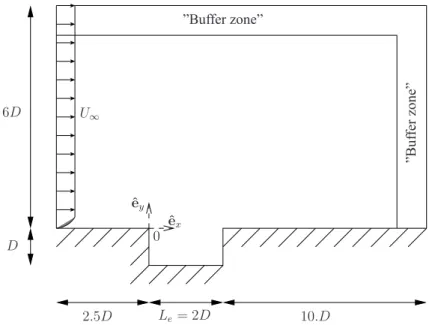
In this section we present the results of validation for the cavity of Le/D ratio of 2. The f ow is initialised by a laminar boundary layer so as to have a thickness ofδ/D = 0.28at the leading edge of the cavity. The Reynolds number of the f ow based on the cavity depth is1500and the f ow Mach number is0.6 as inRowleyet al.(2002). The representative f ow in our case is laminar due to the restriction of computational resources for a real time turbulent simulations. Also it is worthwhile to use scale down the problem to laminar regions to test the basic developments. The computational domain consists of14Din the stream-wise direction and7Din the vertical direction. The cavity f ow conf guration is as shown in f gure1.1. For the mesh a double hyperbolic tangent distribution is used in both the stream-wise and vertical directions, with a stretch ratio of 5%. The inf uence of mesh

ˆ e_x ˆ e_y

0

Le= 2D D

U∞

”Buffer zone”

”Bufferzone”

6D

2.5D 10.D

Figure 1.1 -Schematic diagram of cavity configuration and computational domain.

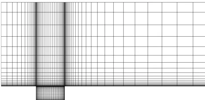
resolution on numerical results is measured by performing a mesh convergence studies to obtain grid independent results. The different mesh sizes used in the studies is given in table 1.1. The typical mesh used in this study is shown in f gure1.2and corresponds to mesh M.

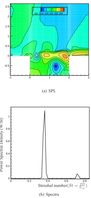
Figure1.3 shows the instantaneous contours of vorticity, the size of the recirculation zone being the same order as the depth. Figure 1.4(a) shows the overall sound pressure level (SPL) for the acoustic f eld above the cavity. The maximum SPL is about 170dB at a point near the downstream edge.

This is lower than the value reported inRowleyet al.(2002) where a value of180dB is reported.

This may be due to the artifact of the numerical scheme used in computation which is 4^th order accurate in the present study whereas it is6^thorder accurate in the case ofRowleyet al.(2002). The SPL levels is however is in agreement with the experimental results ofKrishnamurthi(1956) where a typical value of around168dB is reported.

(25)

Mesh Type Block 1 Block 2 (cavity) CFL

Coarse (C) 185×80 60×40 0.75

Medium (M) 260×80 102×80 0.6

Fine (F) 335×108 120×100 0.6

Table 1.1 -Mesh sizes used in computation.

The spectra corresponding to the normal component of velocity at a point in the shear layer is shown in Figure1.4(b) and shows a single frequency. The value of Strouhal number isSt2 = ^f_U²_∞^L = 0.72in good agreement with the value of0.74determined by the Rossiter’s formulaDelprat(2006)

St= (n−0.25)

(M+ 1/0.57) for n= 2

Figure 1.2 -Typical mesh used in cavity corresponding to M in table1.1. One in every fourth cell is plotted.

(26)

1.6. Modelling cavity f ows using NIGLO

0 1 2 3

-1 -0.5 0 0.5 1 1.5 2

vort: -5 -1.665 1.67

(a)

0 1 2 3

-1 -0.5 0 0.5 1 1.5 2

vort: -5 -1.665 1.67

(b)

0 1 2 3

-1 -0.5 0 0.5 1 1.5 2

vort: -5 -1.665 1.67

(c)

0 1 2 3

-1 -0.5 0 0.5 1 1.5 2

vort: -5 -1.665 1.67

(d)

Figure 1.3 -Instantaneous snapshots of vorticity.15contours in the range ^ωD_U ∈[−5,1.67]are plotted. Only a small portion of the computational domain near the cavity is shown.

(27)

-1 0 1 2 3

-0.5 0 0.5 1 1.5 2 2.5

spl: 152 156 160 164 168

(a) SPL

0 0.2 0.4 0.6 0.8

0 0.2 0.4 0.6 0.8 1

PowerSpectralDensity(W/St)

Strouhal number(St= _U^{f D}_∞) (b) Spectra

Figure 1.4 -SPL and spectra of the normal component of velocity aty= 0andx= 1.8Din the shear layer.

(28)

1.7. Introduction of control

Jet upstream

Jet Cavity upstream

Jet Cavity Downstream

(a)

Full Impact Partial Impact No Impact

(b)

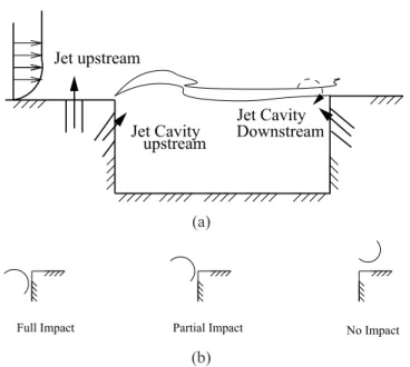
Figure 1.5 -Schematic representation of the action of jet and its effect on the impingement of the shear layer.

1.7 Introduction of control

The control of the cavity is achieved by means of a synthetic jet, which is achieved by modifying the boundary condition in a suitable way. The introduction of control by means of the synthetic jet has been previously performed byShutianet al.(2007) for the case of f ow separation around an airfoil, Kestens(1999) and Samimyet al.(2007) for the case of the cavity. for the experimental control of cavity.

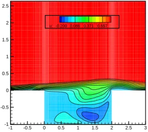
The basic physics behind the control of cavity resonance is to def ect the shear layer from imping- ing on the downstream edge of the cavity thereby arresting the feedback mechanism. As a result of the jet the shear layer can impinge on the downstream edge either fully, partially or can just pass over without any impingement as shown in f gure1.5. Different positions of the jet has been tried, and the position just before the upstream edge of the cavity proves to be more effective. This can be explained by measuring the sensitivity of the f ow, where the upstream edge is more sensitive to external f ow disturbances as shown inMoret-Gabarro(2009). The forcing is typically of the formAsin(ωt), and the actuation is introduced just before the leading edge of the cavity (x∈[−0.15;−0.05]andy= 0), the length of actuation is dependent on cost factors, such as the cost of the actuator in case of experiments or the computational cost in case of numerical simulation. The snapshots of the stream wise component of velocity is shown in f gure1.6, showing the case of no impact and partial impact of the shear layer on the trailing edge.

(29)

-1 -0.5 0 0.5 1 1.5 2 2.5 3

-1 -0.5 0 0.5 1 1.5 2 2.5

u: -0.200 0.086 0.371 0.657

(a) No impact of shear layer on the downstream edge.

-1 -0.5 0 0.5 1 1.5 2 2.5 3

-1 -0.5 0 0.5 1 1.5 2 2.5

u: -0.200 0.086 0.371 0.657

(b) Partial impact of the shear layer on the downstream edge.

Figure 1.6 -Instantaneous snapshots of the stream wise component of velocity depicting the effect of actuation. The forcing is introduced atx∈[−0.15;−0.05]andy= 0and is of the form0.2 sin(0.4t).

(30)

1.8. Conclusion

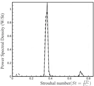
The spectra for a typical forcing of the formAsin(ωt)is shown in the f gure 1.7, Here the peak

0 0.2 0.4 0.6 0.8

0 0.2 0.4 0.6 0.8 1

PowerSpectralDensity(W/St)

Strouhal number(St= _U^{f D}

∞)

Figure 1.7 -Spectra aty= 0andx= 1.8Din the shear layer for the normal component of velocity for the actuated flow (dashed line). The forcing is of the form0.2 sin(0.4t). The spectra is compared for flow without

any actuation (solid line).

corresponding to the Rossiter mode is reduced. One of the objects of the current work is to determine the optimal forcing frequency and amplitude by utilising a reduced order model and check its effect by introducing it in the DNS code.

1.8 Conclusion

In this chapter we have introduced the basic numerical tool used in this study with respect to the governing equations, numerical discretisation and the various boundary conditions used. The code has been validated for the cavity f ow conf guration and will be used through in this study. Introduction of control by means of a synthetic jet at the upstream edge of the cavity, where the f ow is more sensitive to perturbations is performed. The associated spectra shows a decrease at the peak Rossiter mode followed by the appearance of new peaks suggesting the need for optimal criteria for injection.

Various tools to perform the optimal control using ROM will be developed in the subsequent chapters.

(31)

(32)

Chapter 2 Basic tools from control theory

Introduction

Ce chapitre présente brièvement les différentes théories du contrôle actifBewley & Agarwal(1996), Bewley & Liu(1998),Kim & Bewley(2007),Bagheriet al.(2009b) qui ont trouvé des applications en mécanique des fluides lors de ces 15 dernières années, et qui sont utilisées en partie dans ce travail.

On qualifie en premier lieu le type de contrˆole en fonction de la loi de contrˆole et de son action.

On parle de contrôle en boucle ouverte (open loop) lorsque la loi de contrôle est déterminée opti- malement pour stabiliser un système initialement instable. La loi n’est pas modifiable au cours du processus de contrôle. A l’opposé, dans le contrôle en boucle fermée (close-loop), une loi de re- tour (feedback) lie le contrôle à l’état réel et réactualisé du système, assurant une stabilisation plus efficace.

Avant de chercher une loi de contrôle, on doit aussi regarder les aspects de contrôlabilité (ou com- mandabilité) et d’observabilité. La contrôlabilité qualifie la capacité du système à atteindre un état souhaité à partir d’une certaine loi de contrôle et d’une bonne condition initiale. La stabilisabilité, associée à la contrôlabilité, assure qu’il existe une loi de retour capable de stabiliser le système.

Cela revient à dire que les modes non commandables sont tous stables. Enfin l’observabilité, qui mathématiquement est une notion duale à la notion de contrôlabilité, indique que l’observation des entrées et sorties du système, pendant un intervalle de temps fini, permet de retrouver l’état initial et donc l’état complet.

Contrˆole des ´ecoulements en boucle ouvert et optimisation sous contrainte

Un problème de contrôle est bien posé si on peut clairement définir :

• la variable d’´etat du syst`emeφ.

• la variable de contrˆolec.

(33)

2. Basic tools from control theory

• une fonctionnelle coût à minimiserJ(φ, c), associée à la recherche d’une réduction de traˆınée ou de bruit, par example.

• des contraintesF(φ, c) = 0, qui sont les équations d’état avec les conditions aux limites ou initiales éventuellement.

Pour minimiser la fonctionnelle coût, on introduit une fonctionnelle Lagrangienne qui, à la fonc- tionnelle coût, ajoute les contraintes multipliées scalairement par des multiplicateurs de Lagrange ξ, qui sont en réalité des variables d’un problème adjoint restant à définir. La minimisation de la fonctionnelle Lagrangienne se fait en calculant les dérivées de Fréchet par rapport à une variation de l’étatφ, qu’on annule par la suite. Une fois les gradients de la fonctionnelle calculés, on utilise une méthode itérative pour aboutir au contrôle optimal, solution de notre problème. Le calcul des gradients peut aussi être effectué en appliquant la méthode des sensibilités. Il s’agit alors de dériver les contraintes par rapport à la variable de contrôle pour aboutir à la résolution directe d’un système où les dérivées sont les variables principales. Finalement, une discussion sur les intérêts et les in- convénients entre les deux approches conclut cette section :

• différentiation puis discrétisation : en différentiant le système et ses contraintes, on obtient les gradients continus. Ensuite on discrétise l’ensemble du problème pour obtenir la solution numérique.

• discrétisation puis différentiation : on discrétise l’ensemble du problème (contrainte, fonction- nelle), puis on cherche les gradients des grandeurs discrètes par différentiation des équations discrètes.

Contrˆole en boucle ferm´ee

Dans cette partie est développée l’approche classique du contrôle optimal avec loi de retour. A partir de mesure des sorties du système, on estime l’état du système optimalement. C’est l’observation et l’estimation. Ensuite, on suppose que l’état estimé est l’état réel, et on bâtit la loi de contrôle, c’est l’étape de contrôle.

Contrôle linéaire quadratique régulier (LQR)

On considère dans un premier temps un système dans le cadre d’information complète, c’est-à-dire, qu’on peut connaˆıtre à tout instant l’état du système. Par l’approche adjointe on obtient facilement une loi de contrôle de retour (rétroaction) fonction linéairement de l’état, en minimisant une fonc- tionnelle basée sur l’état et le coût du contrôle. La solution est en fait obtenue en résolvant une

équation de Riccati stationnaire, ce qui signifie qu’on cherche à stabiliser le système sur un horizon infini (t → ∞).

Dans une second étape, sur la base des mesures en sortie, on cherche à reconstruire l’état. Pour cela on applique la théorie du filtre de Kalman-Bucy qui suppose que statistiquement le système est soumis à des bruits gaussiens qui engendrent une erreur dans les mesures. Cette erreur se traduit