Combining measured sites, soilscapes map and soil sensing for mapping soil properties of a region

HAL Id: hal-01510132

https://hal.archives-ouvertes.fr/hal-01510132

Submitted on 26 Sep 2017

HAL is a multi-disciplinary open access

archive for the deposit and dissemination of

sci-L’archive ouverte pluridisciplinaire HAL, est destinée au dépôt et à la diffusion de documents

Combining measured sites, soilscapes map and soil

sensing for mapping soil properties of a region

Emily Walker, Pascal Monestiez, Cécile Gomez, Philippe Lagacherie

To cite this version:

Emily Walker, Pascal Monestiez, Cécile Gomez, Philippe Lagacherie. Combining measured sites, soilscapes map and soil sensing for mapping soil properties of a region. Geoderma, Elsevier, 2017, 300, pp.64-73. �10.1016/j.geoderma.2016.12.011�. �hal-01510132�

Version preprint

Combining measured sites, soilscapes map and soil

1

sensing for mapping soil properties of a region

2

W ALKERa _{E., MONEST IEZ}a _{P., GOMEZ}c _{C., LAGACHERIE}b _P. 3

a BioSP, INRA, 84000, Avignon, France

4

b INRA Laboratoire d’étude des Interactions Sol Agrosystème Hydrosystème (LISAH),

5

Campus de la Gaillarde, 2 place Viala, 34060, Montpellier, France

6

c IRD Laboratoire d’étude des Interactions Sol Agrosystème Hydrosystème (LISAH),

7

Campus de la Gaillarde, 2 place Viala, 34060, Montpellier, France

8

Abstract

9

The limited availability of soil information has been recognized as a main

10

limiting factor in Digital Soil mapping (DSM) studies. It is therefore

impor-11

tant to optimize the joint use of the three sources of soil data that can be

12

used as inputs of DSM models, namely spatial sets of measured sites, soil

13

maps and soil sensing products.

14

In this paper, we propose to combine these three inputs, through a

cok-15

riging with a categorical external drift (CKCED). This new interpolation

16

technique was applied for mapping seven soil properties over a 24.6 km2 17

area located in the vineyard plain of Languedoc (Southern France), using

18

an hyperspectral imagery product as example of a soil sensing data.

Cross-19

validation results of CKCED were compared with those of five spatial and

20

non-spatial techniques using one of these inputs or a combination of two of

21

them.

22

The results obtained in the La Peyne Catchment showed i) the utility of

23

soil map and hyperspectral imagery products as auxiliary data for improving

24

soil property predictions ii) the greater added-value of the latter against the

25

former in most situations and iii) the feasibility and the interest of CKCED in

26

a limited number of soil properties and data configurations. Testing CKCED

27

in case study with soil maps of better quality and soil sensing techniques

28

covering more area and depths should be necessary to better evaluate the

29

benefits of this new technique.

30

Keywords:

31

Digital Soil Mapping, remote sensing, hyperspectral data, kriging, cross

32

*Manuscript

Version preprint

validation, soil map, soil properties

33

1. Introduction

34

Given the relative lack of, and the huge demand for, quantitative spatial

35

soil information to be used in environmental managing and modelling, digital

36

soil mapping (DSM) has been proposed as an alternative to the classical soil

37

surveys for the quantitative mapping of soil properties over regions at

inter-38

mediate (20-200m) spatial resolutions (McBratney et al., 2003). McBratney

39

et al. (2003) proposed the equation S = f(s,c,o,r,p,a,n) for summarizing the

40

general principle of DSM. According to this equation, a soil property (S) can

41

be predicted by a spatial inference function (f) using, as input, the existing

42

soil information (s), the spatial covariates that map the different factors of

43

soil formation early defined by Jenny (1941) (c,o,r,p,a,) and the

geograph-44

ical location (n) that can highlight any spatial trends missed by the other

45

covariates.

46

It has been early stressed that the limited availability of the soil

infor-47

mation (the s component) was a severe limiting factor in DSM applications

48

(Lagacherie, 2008). Up to now, most of the soil information used as input in

49

DSM for mapping soil properties has been either soil maps or spatial

sam-50

pling of sites with measured soil properties. When available under the form

51

of soil databases (Rossiter, 2004), the former may provide estimates of soil

52

properties over larger areas with however limited spatial resolutions and

ac-53

curacy (Marsman and de Gruijter, 1986, Leenhardt et al., 1995, Odgers et

54

al., 2012). Pedometricians have developed a large range of algorithms for

ex-55

ploiting spatial sampling of sites for mapping soil properties, using sites with

56

measured soil properties combined with spatial covariates (Oliver and

Web-57

ster, 1989). Recent operational applications of DSM are converging toward

58

the use of regression kriging (Malone et al., 2009; Hengl et al., 2015) in which

59

the two sources of soil data are used together, soil map as a soil covariate

60

among others and spatial sampling with measured soil properties as input

61

data for calibration of the regression model and for spatial interpolation of

62

the regression residuals. However, in situations of sparse spatial sampling

63

that often occurs in operational DSM, the performances of the regression

64

kriging remain severely limited (Vaysse and Lagacherie, 2015).

65

The spatial estimations of soil properties produced by Soil Sensing are a

66

third type of soil information that may be considered also as a DSM input

Version preprint

that may mitigate the dearth in soil data. A growing number of sensors is

68

now available for producing very high resolution (< 5 m) images of estimated

69

soil properties, either by field-based (or proximal) soil sensing techniques

70

(Adamchuk and Rossel, 2011, Mouazen et al, 2007) or by airborne sensing

71

techniques (Selige, 2006; Stevens et al, 2008; Gomez et al, 2008). However,

72

these soil sensing products are most often available over uncompleted and

73

scattered areas because of their high costs and of their limited conditions of

74

application. This prevents from using them as soil covariates in a classical

75

regression kriging approach. As an alternative for mapping soil properties

76

over a region with soil sensing products, we proposed a co-kriging approach

77

(Lagacherie et al, 2012) that combined such input with a spatial sampling of

78

measured sites. By taking hyperspectral-based estimations of clay content

79

over a limited set of fields with bare surfaces as an example of soil sensing

in-80

put, we showed that soil sensing could bring a significant increase of accuracy

81

of clay content predictions over a whole region.

82

In this paper, we went a step further by developing and testing a new

krig-83

ing approach, namely cokriging with a categorical external drift (CKCED),

84

which combines the three possible soil inputs - soil map, spatial sampling

85

of measured sites and soil sensing products -. This approach was compared

86

with spatial and non-spatial techniques using one of these inputs or a

com-87

bination of two of them. The comparisons were performed for seven soil

88

properties (Clay, silt, sand, Calcium Carbonate, pH, Total Iron and CEC)

89

mapped over a 24.6 km2

area located in the vineyard plain of Languedoc

90 (Southern France). 91 2. Case study 92 2.1. Study area 93

The study was carried out in the La Peyne catchment (Figure 1) in the

94

South of France 43o₉′₀′′_{N and 3}o₂′₀′′ _{E. Vineyards form the primary land} 95

use in the area. Marl, limestone and calcareous sandstones from Miocene

96

marine and lacustrine sediments formed the parent material of several soil

97

types observed in this area, including Lithic Leptosols, Calcaric Regosols and

98

Calcaric Cambisols (WRB soil classification, ISSS-ISRIC-FAO, 1998). These

99

sediments were partly covered by successive alluvial deposits ranging from the

100

Pliocene to Holocene and differed in their initial nature and in the duration

101

of weathering conditions. These sediments have produced an intricate soil

102

pattern that includes a large range of soil types, such as Calcaric, Chromic

Version preprint

and Eutric Cambisols, Chromic and Eutric Luvisols and Eutric Fluvisols

104

(Coulouma et al 2008). The local transport of colluvial material along the

105

slopes has added to the complexity of the soil patterns. An earlier ground

106

sampling made in the study region (Lagacherie et al., 2008) showed that these

107

complex soil patterns correspond to a great variability of clay content at the

108

soil surface (from 65 g.kg−1_{to 452 g.kg}−1_{). A study area of 24.6km}2

(Figure

109

1) was defined by intersecting this region of interest with the hyperspectral

110

image used in this study.

111

2.2. Data

112

2.2.1. Spatial sampling of measured sites

113

143 sites (average sampling density of 1 site / 17 ha) were sampled in the

114

study area for measurements of soil properties. All of these samples were

115

composed of five sub-samples collected to a depth of 5 cm for representing a

116

5 meters x 5 meters square. The geographical position at the centre of this

117

square was recorded by a decimetric GPS instrument. After homogenization

118

of the sample, and removal of plant debris and stones, sieving and air

dry-119

ing, about 20 g was devoted to soil properties laboratory analysis. Seven

120

soil properties for which previous estimations from hyperspectral data were

121

attempted (Gomez et al, 2012a) were determined using classical

physico-122

chemical soil analysis (Baize, 1988): calcium carbonate content (CaCO3),

123

clay content (granulometric fraction ≺ 2 µm), silt content (granulometric

124

fraction between 2 to 50 µm), sand content (granulometric fraction between

125

0,05 and 2mm), free iron content, cation-exchange capacity (CEC) and pH.

126

Two subsets of sites can be distinguished among the set of 143 sites. 95

127

sampled sites were located in the bare soil fields. Both soil properties

mea-128

surements and hyperspectral data suitable for estimation of soil properties

129

were available for these 95 sites (Figure 1 left). The remaining 48 sites had

130

soil content measurements but unsuitable hyperspectral data because they

131

were located in vineyard fields covered by vegetation. Both subsets were

132

sampled for obtaining an even spatial distribution of sites while respecting

133

the relative importance of the soil mapping units delineated by Coulouma et

134

al (2008). It must be noted that the criteria of selection of the two subsets of

135

sites (bare soil vs vegetated fields) was totally independent from the spatial

136

distribution of soils, which therefore did not generate any sampling bias.

Version preprint

2.2.2. Soil map

138

The soil map was derived from a very detailed soil map of the study

139

area (Coulouma et al, 2008) by an expert-based grouping of the initial soil

140

units into seven soilscapes as homogeneous as possible regarding the topsoil

141

properties focused in this study. These soilscapes were described in details

142

in Gomez et al. (2012a). The grouping into soilscapes was necessary for

143

obtaining soil mapping units that included a number of sites large enough

144

for applying the tested geostatistical procedures.

145

2.2.3. Airborne HYMAP image and its derivative

146

The HYMAP airborne imaging spectrometer measured reflected radiance

147

in 126 non-contiguous bands covering the 400 – 2500 nm spectral range with

148

around 19 nm bandwidths and average sampling intervals of 17 nm in the

149

400 – 2500 nm domain (http://www.intspec.com/). The HYMAP image

150

was acquired on 13 July 2003 from a 3000 m altitude, providing a 5 x 5 m

151

spatial resolution. Radiometric calibration was performed inflight (Richter,

152

1996) using nadir ground measurements (Beisl, 2001). The ATCOR4 code

153

for airborne sensors was used for atmospheric corrections (Richter and Schl

154

¨

apfer, 2000). Topographic corrections were performed with a high-resolution

155

digital elevation model from the Institut Géographique National (www.ign.fr)

156

and DGPS ground control points.

157

The image was masked by using NDVI to remove living vegetation

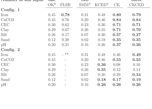
(es-158

sentially vineyards). The cellulose absorption band (2010 nm) was used to

159

remove dry vegetation. Small areas of bare soils located at the parcel margins

160

or along roads and pathway were also removed since they were not judged as

161

representative of the neighbouring soil surfaces. Finally, the image provided

162

usable data over 33 690 pixels covering 3.5% of the total area only, that is

163

the 192 bare soil fields that were randomly scattered over the region at the

164 date of measurement. 165 3. Methods 166 3.1. Experimental set-up 167

We present hereafter the general workflow of our testing (Figure 2). The

168

details on methods are presented further.

169

The new algorithm combining the three possible types of soil

informa-170

tion (CKCED) was compared with five non spatial and spatial methods

171

that involved less types of soil information (Figure 2). Ordinary Kriging

Version preprint

(OK) and Partial-Least-square-Regression (PLSR) were applied for

provid-173

ing estimations of soil properties (denoted products in figure 2) from the

174

spatial sampling of measured sites and from hyperspectral data respectively.

175

Soil Map and spatial sampling of measured sites were combined twice, first

176

by a baseline method that consists in computing a mean per soil mapping

177

units (SMM), second by a more sophisticated Kriging with Categorical Drift

178

(KCED, Monestiez et al, 2001). Finally the product derived from

Hyperspec-179

tral (PLSR on figure 2) was combined with the spatial sampling of measured

180

sites using a previously developed co-kriging procedure (CK, Lagacherie et

181

al, 2012)

182

3.2. Non spatial methods

183

Two non spatial methods were applied, namely ’soil mapping unit mean’

184

(SMM) and Partial least Square Regression (PLSR). The former is a trivial

185

method for combining a soil map and a spatial sampling of measured sites.

186

The latter is a well-known regression technique that is widely used in imaging

187

spectrometry (Ben-Dor et al, 2008). We provide a brief description of this

188

method and its application on our case study hereafter. More details can be

189

found in Gomez et al, (2012a).

190

Partial Least Square Regression (PLSR)(Tenenhaus, 1998) is a

regres-191

sion method that allows the management of 1) co-linearity between the

re-192

flectance values at different wavelengths and 2) a number of predictors (here

193

wavelengths) that is larger than the number of samples used for calibration

194

(here measured sites). The principle of PLSR is to project the variables in an

195

area of reduced size defined by a set of orthogonal vectors, called latent

vari-196

ables, that maximize the covariance between the descriptive variables (here

197

the reflectance values at different wavelengths) and the dependent variables

198

(here the soil properties).

199

PLSR was applied to estimate the seven topsoil properties from the 126

200

reflectance bands provided by the Hymap image for all pixels covered with

201

hyperspectral data. The PLSRs were calibrated using data from the

above-202

evoked 95 sites located in the bare soil fields and then applied to the bare soil

203

pixels for estimating the soil properties, including the 95 pixels with measured

204

sites. At this stage the spatial dependences between locations were ignored.

205

It must be also noted that this approach can only be applied for bare soil

206

fields with collocated hyperspectral data.

Version preprint

3.3. Spatial methods

208

The spatial method applied in this study was a bivariate Cokriging with

209

categorical external drift (CKCED). It combines data of soil properties

mea-210

sured on sampling sites (primary variable), hyperspectral data from soil

211

data predicted from hyperspectral imagery with PLSR (the secondary

vari-212

able) and the soilscapes map (categorical external drift known everywhere).

213

CKCED was compared with other spatial methods that only use one -Ordinary

214

Kriging (OK)- or two - Kriging with a Categorical External Drift (KCED),

215

cokriging (CK)- inputs. CKCED, KCED and CK are presented hereafter.

216

3.3.1. Variographic analyses

217

For each soil property, a linear co-regionalization model (Wackernagel

218

1995) was built for the pair "measured value of soil property" and "PLSR

219

HYMAP estimated value of soil property". A difficulty was to take into

220

account the huge difference between the number of these two data. So the

221

cross-variograms were calculated and fitted on the set of 95 bare-soil field sites

222

at which the two variables were available. The two direct semi-variograms

223

were first modelled as linear combinations of two graphically selected basic

224

structures (spherical 300 m and spherical 2300 m) that were found suitable

225

for all the properties. The same basic structures were then fitted to the

226

cross-semi-variograms under the positive semi-definite constraint(Goovaerts,

227

1997). The fits were checked on simple variograms computed on full hymap

228

dataset (see Figure 3).

229

3.3.2. Neighbourhood selection

230

To limit the size of the cokriging system and its unbalanced block

struc-231

ture (33690 vs 95), it was necessary to sample the hymap sites in a

neighbour-232

hood of the kriged site x0. To preserve short and longer range effects, and 233

due to patchy structure of hymap data, a trial-and-error approach produced

234

the following trade off: all hymap sites were kept within a distance of 50 m

235

from x0 (grid lag = 5 m), one over four within a distance of 500 m (grid lag 236

= 10 m) and finally, one over sixteen within a distance of 1500 m (grid lag =

237

20m). The resulting number of selected neighbours was in most case lower

238

than one thousand and at least greater than two hundred. Considering soil

239

sample sites (95), all sites were kept for cokriging in a unique neighbourhood

240

mode (see Figure 4).

Version preprint

3.3.3. Statistical modelling for kriging

242

The variable of interest, i.e. one of the above soil properties, is modelled

243

by a random function Z(x) where x denotes the location index (vector of

244

coordinates). Z(x) is decomposed into a deterministic unknown drift m(x)

245

and a stationary zero-mean random function ZR(x) assumed to be Gaussian 246

distributed. In the kriging with external drift approach, m(x) is modelled as

247

a linear function of a deterministic external variable. In the kriging with

cate-248

gorical external drift (KCED) proposed by Monestiez et al. (1999; 2001) and

249

used here, m(x) is modelled as a set of values ek, k = 1, . . . , p, correspond-250

ing to the five soilscape classes (p = 5). The values ek may be unknown, 251

but the spatial partition of the domain in soilscape classes must be known

252

everywhere. The model can be written as

253 Z(x) = p X k=1 1{k}(x) ek + ZR(x) (1)

where ek is a mean effect for class k to be estimated and 1{k}(x) is the 254

indicator function of the class k: it is equal to one if x is in class k, and it

255

is equal to zero otherwise. The variable Z was sampled at ni sites xi, for 256

i= 1, . . . , ni. (ni = 95). The second variable Y (x), i.e. the covariate of the 257

bivariate cokriging, denoted further CK, which is here the predicted property

258

by PLSR, is modelled on the same way.

259 Y(x) = p X k=1 1{k}(x) ek+ YR(x) (2)

By construction of the PLSR estimates, the mean ek is the same for Y 260

and Z. The variable Y was sampled at nj sites xj, for j = 1, . . . , nj and 261

where nj is the number of neighbours selected among the 33690 HYMAP 262

pixels.

263

To simplify notation in the following, the covariance function of Z for a

264

pair of points CZZ(xi−xi′) is noted C_i,i(ZZ)′ and the cross-covariance between 265

Z and Y , CZY(xi−xj) is noted Ci,j(ZY). 266

Covariances and cross-covariances are directly derived from fitted

vari-267

ograms and co-variograms. Similarly, Z(xi) and Y (xj) are respectively noted 268

Zi and Yj. 269

Version preprint

3.3.4. Kriging with external drift

270

Following Monestiez et al. (1999), the KCED predictor is given by :

271 Z∗(x0) = ni X i=1 λiZi (3)

where the λi’s solve the following kriging system with ni+ p equations to 272

ensure unbiasedness and minimisation of the MSE:

273            ni X i′=1 λi′C_i,i(ZZ)′ − p X k=1 µk1{k}(xi) = Ci,0(ZZ) for i = 1, . . . , ni ni X i=1 λi1{k}(xi) = 1{k}(x0) for k = 1, . . . , p (4) 3.3.5. Cokriging 274 The cokriging CK 275 Z∗(x0) = ni X i=1 λi Zi+ nj X j=1 λ′_j Yj, (5)

where the λi’s and λ′j’s solve the following cokriging system with ni+nj+2 276

equations to ensure unbiasedness and minimisation of the MSE:

277                        ni X i′=1 λi′C_i,i(ZZ)_′ + nj X j=1 λ′_jC_i,j(ZY)− p X k=1 µk = Ci,0(ZZ) for i = 1, . . . , ni nj X j′=1 λ′_j′C (YY) j,j′ + ni X i=1 λiCi,j(ZY)− p X k=1 µk = Cj,0(ZY) for j = 1, . . . , nj ni X i=1 λi = 1 and nj X j=1 λ′_j = 0 (6)

3.3.6. Cokriging with categorical external drift

278

The cokriging with categorical external drift (CKCED) predictor is

for-279

mally the same as an Universal Cokriging, and the has the same Z∗_(x 0) 280

Version preprint

expression where the λi’s and λ′j’s solve the following cokriging system with 281

ni+ nj+ p equations to ensure unbiasedness and minimisation of the MSE: 282                        ni X i′=1 λi′C_i,i(ZZ)′ + nj X j=1 λ′_jC(ZY) i,j − p X k=1 µk1{k}(xi) = Ci,0(ZZ) for i = 1, . . . , ni nj X j′=1 λ′_j′C (YY) j,j′ + ni X i=1 λiC (ZY) i,j − p X k=1 µk1{k}(xj) = C (ZY) j,0 for j = 1, . . . , nj ni X i=1 λi1{k}(xi) + nj X j=1 λ′_j1{k}(xj) = 1{k}(x0) for k = 1, . . . , p (7)

Compared to the previous bivariate cokriging system, the constraints on

283

λ’s and λ′_{’s are summed up considering Z and Y have same theoritical mean} 284

ek for each class k. To get a kriging prediction free from class effects ek, p 285

constraints are necessary so that the sum of weights for the class to whom x0 286

belongs must be one, and the sum of weights in all other classes must be 0.

287

As a consequence, the unit sum on all λ’s : Pni i=1λi+

Pnj

j=1λ′j = 1 is directly 288

obtained by summing the p constraints.

289

There are p Lagrange parameters µ1 to µ_p. Only one term µ, the one 290

corresponding to the class at x0, remains in the kriging variance whose ex-291 pression is : 292 σ_K2(x0) = C0(ZZ),0 − ni X i=1 λiCi,0(ZZ)− nj X j=1 λ′_jC(ZY) j,0 + p X k=1 µk1{k}(x0). (8) 3.4. Validation 293

To assess the performance of spatial predictions, a leave-one-out cross

294

validation R2

CV was calculated. Two distinct data configurations were con-295

sidered for the comparisons of these methods, whether the predicted site was

296

located in a bare soil field with collocated hyperspectral data or not. In the

297

available data set of measured sites, these two configurations corresponded

298

to 95 and 48 sites respectively. Because the aim of this paper was to compare

299

DSM models that used different combinations of input data it was however

300

preferable to validate each model with the same dataset. Furthermore,

be-301

cause of the low number of the latter, the specific locations of the sites could

302

have hampered the comparisons between methods and data configurations.

Version preprint

which would have made comparisons less effective. Therefore we tested the

304

methods in the two data configurations from the same set of 95 sites. For

305

these sites we obtained the absence of collocated hyperspectral data by

re-306

moving all hymap data of the bare soil plot to whom belongs the prediction

307

point. We however kept the whole set of sites (143) for testing the Ordinary

308 kriging. 309 4. Results 310 4.1. Co-regionalization models 311

The fitted models are composed of two spherical models for ranges of

312

300 m and 2300 m. The sills for both models were estimated for simple

313

variograms and crossed variograms, as described in the table ??.

314

As shown by the examples of fitted variograms for three representative

315

soil properties (Figure 3) acceptable fits were obtained. As expected, smaller

316

sills were obtained from PLSR HYMAP data than from measured values, the

317

former being unable to capture the whole soil variability. Table ?? exhibited

318

also contrasted 300 m sill / 2300 m sill ratio across soil properties. The

319

largest ones, i.e. the largest proportions of "local" variability, were observed

320

for CaCO3 and Iron whereas textural properties and CEC had the smallest

321

ones. pH represented an intermediate situation.

322

4.2. Performance of estimation techniques

323

Table 2 shows the performances of the six estimation techniques using

324

various number of soil inputs, for the seven soil properties of interest and for

325

two data configurations, namely collocated HYMAP data vs no collocated

326

HYMAP data but with hymap data in the neighbourhood. All the results

327

are expressed in R2 _{calculated by cross-validation over the subset of 95 sites} 328

for which all the estimation techniques can be tested (see section ??).

329

Spatial estimation techniques that combined soil inputs (KCED, CK or

330

CKCED) generally outperformed estimation techniques using a single

in-331

put (OK, PLSR) or non-spatial combination of measured sites with a soil

332

map (SMM). However, in the case of collocated hymap data, the

improve-333

ment was only moderate for iron, which had already good performances with

334

PLSR. Moreover, in the case of no collocated hymap data, combining

mea-335

sured sites and hymap outputs (CK) even produced a decrease in prediction

336

performances for Clay and CEC.

Version preprint

Combining measured sites with either the soil map (KCED) or the hymap

338

data (CK) had contrasted interests across soil properties and data

configura-339

tions. In the case of collocated hymap data, CK clearly outperformed KCED

340

whatever the soil properties, with however greater differences for soil

prop-341

erties having already good results with the Hymap data alone (PLSR). In

342

the case of no collocated hymap data, KCED and CK gave similar results

343

for most of the soil properties (iron, silt, sand and pH). However KCED

344

outperformed CK for CEC and Clay whereas CK outperformed KCED for

345

CaCO3. It must be noted that neither the individual performances of the

346

added inputs (PLSR and SMM, table ??) nor the spatial structures of the

347

soil properties (table ??) could explain these differences.

348

The newly developed estimation technique that combined the three soil

349

inputs (CKCED) provided an improvement for only three properties (Iron,

350

silt and sand) in the case of no-collocated hymap data. In all other cases,

351

the performances of CKCED was similar to those of CK. Here again, it was

352

not possible to relate the differences of results across soil properties with the

353

individual performances of the added inputs and the spatial structures of the

354

soil properties.

355

4.3. Mapping

356

Figure 4 shows images of clay, sand and iron obtained from the cokriging

357

with categorical external drift (CKCED) interpolation . The image of clay

358

showed a global increase of clay content from the north to the south of the

359

area. This is probably the effect of the parent materials, the old (Pliocene)

360

fluvial deposits located in the southern part of the area, being more clayey

361

than any other parent materials. The image of sand showed the converse

362

spatial distribution, apart from the south West of the study area where soils

363

formed on limestone out crops had both low clay and low sand contents. The

364

Iron image exhibited a significantly different soil pattern from the previous

365

ones with two distinct iron-rich areas that corresponded to soil formed on

366

Wurm (North) and Pliocene (south) fluviatile deposits. This last image was

367

also the one in which the delineations of the soil map were the most visible.

368

5. Discussion

369

5.1. Case study representativeness

370

Bivariate cokriging and the other interpolation techniques were tested

371

in a Mediterranean area that has been used as a case study for digital soil

Version preprint

mapping and remote sensing for a long time (e.g. Leenhardt et al, 1994

373

; Lagacherie and Voltz, 2000, Lagacherie et al, 2008, Gomez et al, 2012).

374

In spite of its moderate size, it includes a great variety of parent materials

375

and landscape positions that yield complex patterns of soil variations. This

376

was confirmed by the study of variograms of seven soil properties that all

377

exhibited bi-scaled spatial structures and contrasted ratio of short and

large-378

scale variations with properties.

379

In this study, seven soil properties were considered. This allowed

ob-380

serving contrasted situations with regard to the quality of the auxiliary

spa-381

tial data used as input of the interpolation techniques. The proportion of

382

variances captured by the hyperspectral-based estimations of soil properties

383

ranged between R2

= 0.20 for sand to R2

= 0.78 for iron, which corresponds

384

to the range of performances shown in the literature (e.g. Selige et al., 2006;

385

Gomez et al., 2008; Ben-Dor et al, 2008, Stevens et al., 2010). As already

386

observed by Ben Dor et al (2002),the soil properties that corresponded to

387

a chromophore (here Clay, Iron, CEC and Calcium Carbonate) were

pre-388

dicted with more accuracy than the other soil properties (sand, silt and pH).

389

The range of proportions of variances captured by the soil map was smaller

390

(R2

< 0.31). From the soilmap assessments performed in the same

pedolog-391

ical area (Lennhardt et al, 1994; Vaysse and Lagacherie, 2015), this results

392

correspond to a medium to short scale soil map, that cover substancial

pro-393

portions of land, e.g. 39% in Europe (King and Montanarella, 2012) and

394

11% in Africa (Nachtergaele and van Ranst, 2002).

395

In conclusion, the case study can be considered as matching well the

396

level of availability and quality of DSM soil inputs that can be currently

397

encountered nowadays. However, many regions in the world may include

398

hyperspectral data that cover a larger proportion of the study area and more

399

accurate soil maps. For these regions, better and more contrasted results

400

than those presented in this paper could certainly be expected.

401

5.2. Interest of hyperspectral products as DSM soil input

402

Up to now, the use in DSM of hyperspectral products that may provide

403

soil property estimations at both high resolutions and large extents has been

404

rarely experimented (Schwangart and Jammer, 2011, Lagacherie et al, 2012,

405

Gomez et al, 2012b,), and have never been compared with the more common

406

use of a soil map as a DSM input combined with measured sites (Mc Bratney

407

et al, 2003, Kempen et al, 2011[1]).

Version preprint

The results we obtained showed that hyperspectral products used as an

409

auxiliary input in cokriging generally provided better improvements of soil

410

property predictions than a soil map used as an auxiliary input in

Krig-411

ing with a Categorical external Drift. The only exceptions were for Clay and

412

CEC in locations with no collocated hyperspectral data, for which the

combi-413

nations with the hyperspectral products surprisingly decreased the precisions

414

obtained by simply interpolating the measured sites by Ordinary Kriging.

415

However, the seemingly greater interest of hyperspectral products must

416

be nuanced since we did not have in this case study examples of very

well-417

predicted soil properties by a soil map ( R2 < 0.31). Furthermore, one may

418

remember that hyperspectral products can only deliver estimations of surface

419

soil properties because the effective penetration depths of optical sensors do

420

not exceed several millimetres (Liang, 1997[2]), which limits, at best (i.e.

421

cultivated areas), the soil property predictions to the topsoil horizons only.

422

5.3. Interest of combining three DSM soil inputs

423

We proposed a cokriging with a categorical external drift that allowed

424

combining the two available auxiliary variables - the soil map and the

hyper-425

spectral estimations of soil properties- with the set of measured sites. This

426

new interpolation technique was found interesting in situations with no

collo-427

cated hyperspectral-based estimations and for a limited number of properties

428

(Table 2). These properties were characterized either by the worst

perfor-429

mances of the soilscapes map (silt and sand) or by the best performances

430

of the hyperspectral based predictions (iron). It must be noted that the

431

amount of local variation of the soil properties (table 1) that was expected

432

to decrease the interest of using non-collocated hyperspectral-based soil

esti-433

mations as auxiliary variable did not explain any difference in performances

434

between soil properties. Here again, we did not explore enough variability

435

of soil map precisions and distances to neighbouring hyperspectral situations

436

for identifying clearly the area of interest of CKCED.

437

5.4. Future work

438

The performances of the interpolation techniques tested in this paper

439

could be improved either by better auxiliary spatial variables or by better

440

spatial models.

441

Concerning the former, two ways could be explored. A better accuracy of

442

the soil map can be obtained by increasing its spatial resolution for obtaining

443

a more detailed soil map. However the number of sampled sites can become

Version preprint

a limiting factor since KCED requires a good estimate of the mean value

445

of the property within each soil mapping units, which cannot be obtained

446

without a denser spatial sampling of sites than the one used in this study.

447

Beside, since we observed that much better results were obtained within the

448

bare soil area where hyperspectral estimates of soil property were available

449

without interpolation, it would be worth extending this area. This can be

450

straightforwardly done by a better selection of the date of the fly (Gomez et

451

al, 2012b). Furthermore, the remaining vegetated area can be processed with

452

spectral unmixing (Bartholomeus et al, 2010) or source separation algorithms

453

(Ouerghemmi et al, 2016) for filtering the vegetation signal that may perturb

454

the estimations of soil properties. Finally, other soil sensing techniques than

455

hyperspectral imagery can be used as soil input to enlarge both the area and

456

the exploration depth of the targeted soil properties.

457

The spatial models underlying the interpolations could be improved first

458

by taking into account additional soil covariables like e.g. Digital

Eleva-459

tion Model and its derivatives e.g. slope, aspect, curvature, that have been

460

largely used in Digital Soil Mapping (McBratney et al, 2003). Another way

461

of improvement is to take into account the non stationarity of soil

prop-462

erty variations by applying interpolations based on local (Sun, 2012) and/or

463

anisotropic spatial models (Schwangart and Jammer, 2011).

464

6. Conclusion

465

This study tested the use of the three possible soil inputs for DSM models

466

– spatial set of measured sites, soil map and soil sensing products. A new

467

spatial interpolation technique – cokriging with a categorical external drift –

468

was developed for combining these three inputs. The results obtained in the

469

La Peyne Catchment demonstrated the utility of auxiliary variables such as

470

soil map or hyperspectral imagery products for predicting soil properties and

471

the greater added-value of the latter against the former in most situations.

472

The combination of soilmap and hyperspectral–based estimations of soil

473

property allowed by the novel cokriging with categorical external drift

pro-474

cedure (CKCED) brought improvements for a limited number of soil

proper-475

ties and data configurations. However, to better evaluate its utility, this new

476

combination needs to be tested in other case study with soil maps of better

477

quality and soil sensing techniques covering more area and depths.

Version preprint

7. Acknowledgements

479

This research was granted by INRA, IRD and the French National

re-480

search agency (ANR) (ANR-08-BLAN-0284-01). We are indebted to Dr.

481

Steven M. de Jong, Utrecht University in The Netherlands and to Dr.

An-482

dreas Mueller of the German Aerospace Establishment (DLR) in Wessling,

483

Germany for providing the 2003 HyMap images for this study. We warmly

484

thank the two anonymous reviewers for their constructive and useful

com-485

ments.

486

8. References

487

Adamchuk, V.I., Viscarra Rossel, R.A. 2010. Development of on–the–go

488

Proximal Sensing

489

Systems. In: Proximal Soil Sensing , eds: R.A. Viscarra.Rossel, A.B.,

490

McBratney, B. Minasny, pp 15–28. Progress in Soil Science 1, Springer

491

Dordrecht, Heidelberg, London New York.

492

Bartholomeus, H., Kooistra, L., Stevens, A., Van Leeuwen, M., Van

Wese-493

mael, B., Ben-Dor, E. 2011. Soil organic carbon mapping of partially

494

vegetated agricultural fields with imaging spectroscopy. International

495

Journal of Applied Earth Observation and Geoinformation, 13, 81–88.

496

Beisl U. 2001. Correction of bidirectional effects in imaging spectrometer

497

data. Zurich University, Zurich (Switzerland).

498

Ben-Dor E., Patkin K., Banin A. and Karnieli A. (2002). Mapping of

sev-499

eral soil properties using DAIS-7915 hyperspectral scanner data-a case

500

study over clayey soils in Israel. International Journal of Remote

Sens-501

ing, 23 (6), p. 1043-1062.

502

Ben-Dor, E., Taylor, R.G., Hill, J., Dematte, J.A.M., Whiting, M.L.,

Chabril-503

lat, S. 2008. Imaging spectrometry for soil applications. Advances in

504

Agronomy, 97, 321–392.

505

Ciampalini, R., Lagacherie, P., Monestiez, P., Walker, E., Gomez, C. 2012.

506

Cokriging of soil properties with VisNIR hyperspectral covariates in the

507

Cap Bon region (Tunisia). In: Minasny, B., Malone, B., McBratney,

508

A.B. (Eds.), Digital Soil Assessments and Beyond (). CRC Press. pp.

509

393–398

Version preprint

Coulouma, G., Barthes, J. P., Robbez-Masson, J. M. 2008. Carte des sols

511

de la Basse Vallee de la Peyne. Report and map UMR LISAH (INRA).

512

Gomez, C., Lagacherie, P., Coulouma, G. 2008. Continuum removal versus

513

PLSR method for clay and calcium carbonate content estimation from

514

laboratory and airborne hyperspectral measurements. Geoderma, 148

515

(2), 141–148.

516

Gomez, C., Lagacherie, P., Coulouma, G., 2012a. Regional predictions of

517

eight common soil properties and their spatial structures from

hyper-518

spectral Vis-NIR data. Geoderma 189-190:176–185.

519

Gomez, C., Lagacherie, P., Bacha, S., 2012b. Using Vis-NIR hyperspectral

520

data to map topsoil properties over bare soils in the Cap-Bon Region,

521

Tunisia, in: Minasny, B., Malone, B., McBratney, A.B. (Eds.), Digital

522

Soil Assessment and Beyond. CRC Press, pp. 387?392.

523

Goovaerts, P. 1997. Geostatistics for Natural ResourcesEvaluation. Oxford

524

University Press.

525

Grunwald, S. 2009. Multi–criteria characterization of recent digital soil

526

mapping and modeling approaches. Geoderma 152:195–207.

527

Henderson, B. L., Bui, E. N., Moran, C. J., Simon, D. A. P. 2005.

Australia-528

wide predictions of soil properties using decision trees. Geoderma,

529

124(3–4), 383–398.

530

Hengl, T., de Jesus, J.M., MacMillan, R.A., Batjes, N.H., Heuvelink, G.B.M.,

531

Ribeiro, E., Samuel-Rosa, A., Kempen, B., Leenaars, J.G.B., Walsh,

532

M.G., Gonzalez, M.R., 2014. SoilGrids1km Ñ Global Soil Information

533

Based on Automated Mapping. PLoS One 9, e105992.

534

Jenny, H. 1941. Factors of soil formation (p. 281). New York, NY:

McGraw-535

Hill Book Company.

536

Kempen, B., Brus, D.J., Stoorvogel, J.J., 2011. Three-dimensional mapping

537

of soil organic matter content unsig soil type-specific depth functions.

538

Geoderma 162(1-2), 107-123.

539

King D. and Montanarella L. 2002. Inventaire et surveillance des sols en

540

Europe. Etude et Gestion des Sols, 9: 137–148.

Version preprint

Lagacherie, P., Voltz, M. 2000. Predicting soil properties over a region using

542

sample information from a mapped reference area and digital elevation

543

data: a conditional probability approach. Geoderma, 187–208.

544

Lagacherie, P. 2008. Digital soil mapping: a state of the art. In A. E.

545

Hartemink, A. B. McBratney, M. L. Mendonca Santos (Eds.), Digital

546

soil mapping with limited data (pp. 3–14). Springer science.

547

Lagacherie, P., Baret, F., Feret, J-B, Madeira Netto, J., Robbez-Masson,

548

J.M. 2008. Estimation of soil clay and calcium carbonate using

labora-549

tory, field and airborne hyperspectral measurements. Remote Sensing

550

of Environment, 112 (3), 825–835.

551

Lagacherie, P., Bailly, J.S., Monestiez, P., Gomez, C. 2012. Using scattered

552

hyperspectral imagery data tomap the soil properties of a region. Eur.J.

553

Soil Science; 63:110–119.

554

Leenhardt, D., Voltz, M., Bornand, M., Webster, R. 1994. Evaluating soil

555

maps for prediction of soil water properties. European Journal of Soil

556

Science, 45(3), 293–301.

557

Liang, S., 1997. An investigation of remotely-sensed soil depth in the optical

558

region. International Journal of Remote Sensing 18, 3395Ð3408

559

Malone, B.P., McBratney, A.B., Minasny, B., 2011. Empirical estimates of

560

uncertainty for mapping continuous depth functions of soil attributes.

561

Geoderma 160, 614Ð626.

562

Marsman, B. A., Gruijter, J. J. de. 1986. Quality of soil maps: a comparison

563

of survey methods in a sandy area. Soil Survey Papers, Netherland Soil

564

Survey Institute, Wageningen.

565

McBratney, A. B., Mendonca Santos, M. L., Minasny, B. 2003. On digital

566

soil mapping. Geoderma, 117(1–2), 3–52.

567

Monestiez, P., Allard, D., Navarro Sanchez, I., Courault, D. 1999. Kriging

568

with categorical external drift: Use of thematic maps in spatial

pre-569

diction and application to local climate interpolation for agriculture,

570

in geoENV II: Geostatistics for Environmental Applications ,

Gomez-571

Hernandez J., Soares A. and Froidevaux R. Eds, Kluwer Academic

572

Publishers, Dordrecht, 163–174.

Version preprint

Monestiez, P., Courault, D., Allard, D., Ruget, F., 2001. Spatial

interpo-574

lation of air temperature using environmental context: application to

575

crop model. Environmental and Ecological Statistics. 8: 297–309.

576

Mouazen, A. M., Maleki, M. R., De Baerdemaeker, J., Ramon, H. 2007.

577

Online measurement of some selected soil properties using a VIS–NIR

578

sensor. Soil and Tillage Research, 93(1), 13–27.

579

Mulder, V.L., De Bruin, S., Schaepman, M.E., and Mayr, T.R., 2011. The

580

use of remote sensing in soil and terrain mapping – A review. Geoderma

581

162, 1–19.

582

Nachtergaele, F. O., Van Ranst, E. 2002. Qualitative and Quantitative

583

Aspects of Soil Databases in Tropical Countries. In G. Stoops (Ed.),

584

Evolution of Tropical Soil Science: Past and Future (pp. 107–126).

585

Brussel: Koninklijke Academie voor Overzee Wetenschappen.

586

Odgers, N. P., Libohova, Z., Thompson, J. A. 2012. Equal–area spline

587

functions applied to a legacy soil database to create weighted-means

588

maps of soil organic carbon at a continental scale. Geoderma, 189,

589

153–163.

590

Oliver, M. A., Webster, R. 1989. A geostatistical basis for spatial weighting

591

in multivariate classification. Mathematical Geology, 21(1), 15–35.

592

Ouerghemmi, W., Gomez, C., Naceur, S., Lagacherie, P., 2016. Semi-blind

593

source separation for the estimation of the clay content over

semi-594

vegetated areas using VNIR/SWIR hyperspectral airborne data.

Re-595

mote Sens. Environ. 181, 251–263.

596

Richter, R. 1996. Atmospheric correction of DAIS hyperspectral image data.

597

Computers and Geosciences 22, 785–793.

598

Richter, R., Schlapfer, D.A., 2000. A unified approach to parametric

geocod-599

ing and atmospheric/topographic correction for wide FOV airborne

600

imagery. Part 2: atmospheric Correction. Proc. 2nd Intl. EARSeL

601

Workshop on Imaging Spectroscopy, Enschede, July 11–13, 2000.

602

Rossiter, D. G. 2004. Digital soil resource inventories: status and prospects.

603

Soil use and management, 20(3), 296–301.

Version preprint

Schwanghart, W., Jarmer, T. 2011. Linking spatial patterns of soil organic

605

carbon to topography – a case study from south–eastern Spain.

Geo-606

morphology, 126, 252-263. DOI: 10.1016/j.geomorph.2010.11.008.

607

Selige, T., Bohner, J., Schmidhalter, U. 2006. High resolution topsoil

map-608

ping using hyperspectral image and field data in multivariate regression

609

modeling procedures. Geoderma, 136, no1–2, pp. 235–244.

610

Stevens, A., Udelhoven, T., Denis, A., Tychon, B., Lioy, R., Hoffmann,

611

L., Wesemael, B. 2010. Measuring soil organic carbon in croplands

612

at regional scale using airborne imaging spectroscopy, Geoderma, 158,

613

1–2.

614

Sun, W., Minasny, B., McBratney, A. 2012. Analysis and prediction of soil

615

properties using local regression kriging. Geoderma, 171–172, 16–23.

616

doi:10.1016/j.geoderma.2011.02.010.

617

Tenenhaus M. 1998. La regression PLS. Theorie et Pratique. Editions T,

618

Paris.

619

Vaysse, K., Lagacherie, P. 2015. Evaluating Digital Soil Mapping

ap-620

proaches for mapping GlobalSoilMap soil properties from legacy data

621

in Languedoc Roussillon (France). Geoderma Regional, 4, 20–30.

622

doi:10.1016/j.geodrs.2014.11.003.

623

Wackernagel, H., 1995. Multivariate geostatistics. Springer Verlag Editions.

624

255 pp.

Version preprint

Table 1: Fitted sill and range parameters of direct (samples and hymap) and cross

vari-ograms. *in g2_/kg2_{for clay, CaCO3, Iron, Sand and Silt; no unit for pH; M eq}2_/100g2_for

CEC

Soil property range (m) samples sill* crossed sill* Hymap sill*

Clay 300 3578 1886 1600 2300 1387 1691 2062 CaCO3 300 7522 4819 4658 2300 13412 12871 12352 CEC 300 6.94 4.59 4.51 2300 1.79 1.56 2.03 Iron 300 0.169 0.129 0.141 2300 0.314 0.274 0.245 pH 300 0.338 0.028 0.023 2300 0.366 0.178 0.096 Sand 300 11146 1516 1270 2300 3715 2969 2373 Silt 300 7910 1586 1081 2300 249 504 1021 Table

Version preprint

Table 2: Performances (cross validation R2) of the different methods for two data con-figurations: with collocated hymap data (Config. 1) and with no collocated hymap data

but with hymap data in the neighbourhood(Config. 2). OK: Ordinary Kriging, PLSR: Partial least square Regression, SMM : mean per Soil mapping unit, KCED: Kriging with categorical external drift, CKCED: Cokriging with categorical external drift. *insensitive to data configuration (results are repeated for enabling comparisons). ** "-" means "not feasible with this data configuration"

Number of soil input one two three

OK* PLSR SMM* KCED* CK CKCED

Config. 1 Iron 0.45 0.78 0.31 0.48 0.80 0.79 CaCO3 0.45 0.76 0.20 0.46 0.84 0.84 CEC 0.30 0.62 0.23 0.36 0.71 0.71 Clay 0.29 0.67 0.26 0.35 0.71 0.70 Silt 0.26 0.17 0.07 0.30 0.37 0.37 Sand 0.12 0.20 0.02 0.18 0.35 0.35 pH 0.20 0.31 0.16 0.26 0.37 0.36 Config. 2 Iron 0.45 - ** 0.31 0.48 0.46 0.49 CaCO3 0.45 - 0.20 0.46 0.55 0.55 CEC 0.30 - 0.23 0.36 0.08 0.10 Clay 0.29 - 0.26 0.35 0.12 0.14 Silt 0.26 - 0.07 0.30 0.29 0.34 Sand 0.12 - 0.02 0.18 0.17 0.19 pH 0.20 - 0.16 0.26 0.26 0.26

Version preprint

Figure 1

Version preprint

!

!

"

!

!

"

Version preprint ● ● ● ● ● ● ● ● ● ● ●

0

500

1000

1500

2000

0

1000

2000

3000

4000

5000

distance (m)

gamma (samples)

Clay

0

500

1000

1500

2000

−3000

−2000

−1000

0

1000

2000

3000

gamma samples − h

ymap

0

500

1000

1500

2000

0

500

1000

1500

2000

2500

3000

3500

gamma h

ymap

Version preprint ● ● ● ● ● ● ● ● ● ● ●

0

500

1000

1500

2000

0

2

4

6

8

distance (m)

gamma (samples)

CEC

0

500

1000

1500

2000

−6

−4

−2

0

2

4

6

gamma samples − h

ymap

0

500

1000

1500

2000

0

1

2

3

4

5

6

gamma h

ymap

Version preprint ● ● ● ● ● ● ● ● ● ● ● ● ● ● ●

0

500

1000

1500

2000

0.0

0.1

0.2

0.3

0.4

0.5

distance (m)

gamma (samples)

Iron

0

500

1000

1500

2000

−0.4

−0.2

0.0

0.2

0.4

gamma samples − h

ymap

0

500

1000

1500

2000

0.0

0.1

0.2

0.3

0.4

gamma h

ymap

Version preprint

Figure 4