The adaptive Kalman filter and micromechanical inertial instrument performance

THE ADAPTIVE KALMAN FILTER

AND

MICROMECHANICAL INERTIAL INSTRUMENT PERFORMANCE

by

Jonathan Andrew Kossuth

S.B., Massachusetts Institute of Technology (1993) Submitted to the Department of Aeronautics and Astronautics

in Partial Fulfillment of the Requirements for the Degee of

MASTER OF SCIENCE in AERONAUTICS AND ASTRONAUTICS at the

MASSACHUSETTS INSTITUTE OF TECHNOLOGY May 1993

© Jonathan Andrew Kossuth, 1993. All Rights Reserved

Signature of Author

Dep ent of Aeronautics and Astronautics May 7, 1993

Approved by

Paul Steranka Principal Member Technical Staff, Charles Stark Draper Laboratory Thesis Supervisor

Certified by

Accepted by

'

Professor Wallace E. Vander Velde Department of Aeronautics and Astronautics

-.. /a Thesis Advisor

"oL,

L/ Professor Harold Y. Wachman Chairman, Department Graduate Committee

AerO

08

1993

1

At 1,

THE ADAPTIVE KALMAN FILTER AND

MICROMECHANICAL INERTIAL INSTRUMENT PERFORMANCE by

Jonathan Andrew Kossuth

Submitted to the Department of Aeronautics and Astronautics on May 7, 1993

in Partial Fulfillment of the Requirements for the Degree of Master of Science in Aeronautics and Astronautics

ABSTRACT

As newer technologies in inertial instruments emerge, the need for more powerful data analysis techniques is increasing because both unmodeled errors and unknown factors may exist, and must be accounted for, in the instrument data. An online adaptive Kalman filter has been developed for analysis of these inertial instruments using the innovation sequence of the Kalman filter in order to determine the optimal filter parameters.

Performance of the filter is improved by determining the proper system model, by identifying any unknown parameters in the system matrices, or by identifying any periodic noise in the signal. A fault tolerant algorithm is included in the filter. Maximum likelihood techniques are used to estimate the parameters of the filter matrices by choosing those parameter values that maximize the likelihood function of the parameters. Correlation methods are used to determine the proper system model by comparing the innovation sequence to a known signal. Power spectral density analysis is used to identify periodic signals by examining the PSD of the innovation sequence.

Simulations to verify the filter performance have been run successfully for a number of cases. In each of these simulations, the adaptive Kalman filter was able to modify the filter matrices to achieve optimality. The adaptive Kalman filter has been applied to data from various micromechanical gyroscope tests, including a stationary drift test and a commanded rate test. These filters have been used for both raw data reduction and reduced data analysis. By applying these adaptive Kalman filters to micromechanical gyroscope data, real improvements in data analysis have been shown. The raw data reduction adaptive filter improved data decimation by up to 50 percent over a triangular filter. The reduced data analysis adaptive filter produced filter estimates twice as accurate as the traditional Kalman filter, and has identified a pressure sensitivity and a rate squared sensitivity in the micromechanical gyroscope.

Thesis Supervisor: Paul Steranka

Principal Member Technical Staff, C. S. Draper Laboratory Thesis Advisor: Professor Wallace E. Vander Velde

Acknowledgments

I would like to thank Charles Kochakian for his support over the past three years. My sincerest gratitude is extended to my thesis supervisor, Paul Steranka, for his guidance and assistance for the past year. I would like to thank my thesis advisor, Professor Vander Velde, for his insightful comments that helped this thesis come together. I would also like to thank Anthony Kourepenis and Thomas Farnkoff for their assistance in acquiring data, as well as their explanations of micromechanical inertial instrument technology.

I thank my friends at MIT for the help and support that they have given me and for making the past five years at MIT enjoyable. I also thank the people at Draper Lab that made my day to day life interesting. My family, especially my parents, George and Elizabeth Kossuth, deserves tremendous thanks for encouraging me to do my best over the past 23 years. I give special thanks to Kimberly Santagate for her love and friendship over the past five years.

This thesis was researched and written at the Charles Stark Draper Laboratory under Contract IR&D 93-1-357-1.

Publication of this thesis does not constitute approval by the Laboratory of the findings or conclusions contained herein. It is published for the exchange and stimulation of ideas.

I hereby assign my copyright of this thesis to the Charles Stark Draper Laboratory, Inc., of Cambridge, Massachusetts.

Jon an Andrew Kossuth May 7, 1993

Permission is hereby granted by the Charles Stark Draper Laboratory, Inc. to the Massachusetts Institute of Technology to reproduce and to distribute copies of this thesis document in whole or in part.

Table of Contents

1.2 Adaptive Filter Concepts ... 14

1.2.1 Kalman Filter ... 14

1.2.2 Maximum Likelihood Estimator ... 14

1.2.3 Model Adaptive Filter ... ... 15

1.2.4 Periodic Signal Identification... ... 15

1.2.5 Data Analysis Filters ... ... 15

1.3 Data Analysis ... 16

1.3.1 Micromechanical Inertial Instruments ... 16

1.3.2 Data Analysis ... 16

1.3.3 Future Work ... 16

Chapter 2 Kalman Filter Theory ... 17

2.1 History of Estimators ... 17

2.2 Kalman Filter Theory ... 17

2.3 The Innovation Property of an Optimal Filter ... . 19

2.3.1 Innovation Sequence as White Noise in an Optimal Filter ... 19

2.3.2 White Noise Test for Optimality of Kalman Filter ... 21

2.4 Limitations of Kalman Filter... 23

Chapter 3 Maximum Likelihood Estimator ... ... 25

3.1 Motivation for Maximum Likelihood Estimator ... 25

3.2 Maximum Likelihood Estimator ... 25

3.3 Maximum Likelihood Estimator Theory ... 26

3.4 Derivation of the Maximum Likelihood Kalman Filter... 31

3.5 Equations for Maximum Likelihood Kalman Filter ... 34

3.5.1 Approximations for Online Operation ... 40

3.6 Verification of Maximum Likelihood Estimator ... 41

3.6.1 Generation of Simulated Data... ... 42

3.6.1.1 Generation of White Noise Sequences... 42

3.6.1.2 Generation of Random Walk Sequences ... 42

3.7 Results of Simulated Data Analysis ... ... 43

3.8 Conclusions ... 45

Chapter 4 Model Adaptive Filter Using Correlation Methods ... 47

4.1 Model Adaptive Filter ... 47

4.2 Theory of Correlation Functions ... ... 47

4.3 Derivation of Model Adaptive Filter ... ... 48

4.3.1 Implementation of Model Adaptive Filter ... 50

4.4 Verification of Model Adaptive Filter ... ... 51

4.6 Conclusions ... 59

Chapter 5 Power Spectral Density Analysis ... ... 61

5.1 Motivation for PSD Analysis ... ... 61

5.2 Power Spectral Density Theory ... ... 61

5.2.1 Fourier Transforms ... ... ... 62

5.2.2 Power Spectral Density Function for Finite Data Sets ... 63

5.2.3 Discrete Fourier Transforms ... ... 65

5.2.4 Nyquist Criterion and Aliasing ... .... 65

5.3 Filter D esign... ... 67

5.4 Filter Verification... 67

5.4.1 Single and Multiple Frequency Noise... 67

5.4.2 Distributed Frequency Noise ... .... .71

5.4.2.1 Motivation ... 71

5.4.2.2 Approach ... ... 72

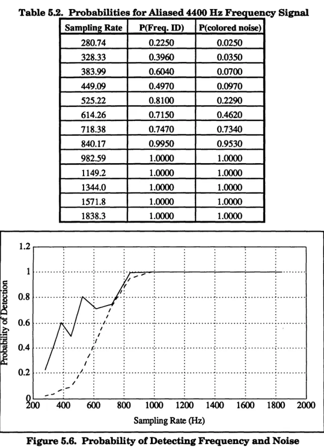
5.4.2.3 Results ... ... 72

5.5 Conclusions ... 77

Chapter 6 Adaptive Data Analysis Filter Development... ... 79

6.1 Introduction ... 79

6.2 Raw Data Reduction Adaptive Filter ... 79

6.2.1 Verification of Raw Data Reduction Filter ... 79

6.2.2 Raw Data Reduction Adaptive Filter vs. Triangular Filter ... 83

6.3 Reduced Data Analysis Adaptive Filter... ... 85

6.4 Conclusions on Adaptive Filters ... 91

Chapter 7 Micromechanical Inertial Instruments... 93

7.1 Introduction ... 93

7.2 Micromechanical Gyroscopes ... ... 93

7.2.1 Vibratory Gyroscope ... 93

7.2.2 Noise Sources ... 96

7.2.3 Inverted Gyroscope ... 96

7.2.4 Tuning Fork Gyroscope ... ... 97

7.3 Conclusions ... 98

Chapter 8 Micromechanical Gyroscope Data Analysis ... 99

8.1 A pproach ... ... 99

8.2 Stationary Drift Test with Original Gyro Design, Test 8A... 99

8.2.1 Raw Data Reduction of 3 Hz Stationary Drift Test ... 99

8.2.2 Reduced Data Analysis of 3 Hz Stationary Drift Test ... 101

8.3 Scale Factor Test with Inverted Gyroscope Design, Test 8B ... 102

8.3.1 Reduced Data Analysis of Commanded Rate Test ... 103

8.4 Stationary Drift Test with Inverted Design, Test 8C ... 106

8.4.1 Raw Data Reduction of 1500 Hz Stationary Drift Test ... 107

8.4.2 Reduced Data Analysis of 1500 Hz Stationary Drift Test ... 107

8.5 Pressure Variation Test for Inverted Design ... ... 109

8.6 Commanded Rate Test for Original Design... 111

8.7 Conclusions ... 112

Chapter 9 Conclusions ... 113

9.1 Results ... 113

9.2 Implementation of Adaptive Filters ... 114

9.3 Recommendations for Future Work... 114

References ... 115

List of Figures

Figure 2.1. Descriptions of White Noise Properties ... 21

Figure 3.1a. Estimate Intervals at Every Sample Time... 26

Figure 3. lb. Estimate Intervals at Every N Sample Times ... 26

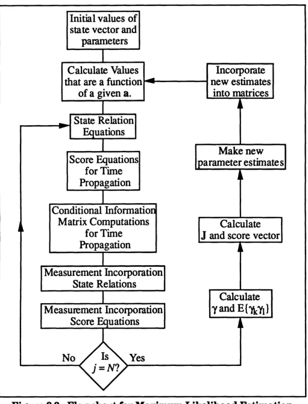
Figure 3.2. Flowchart for Maximum Likelihood Estimation... 35

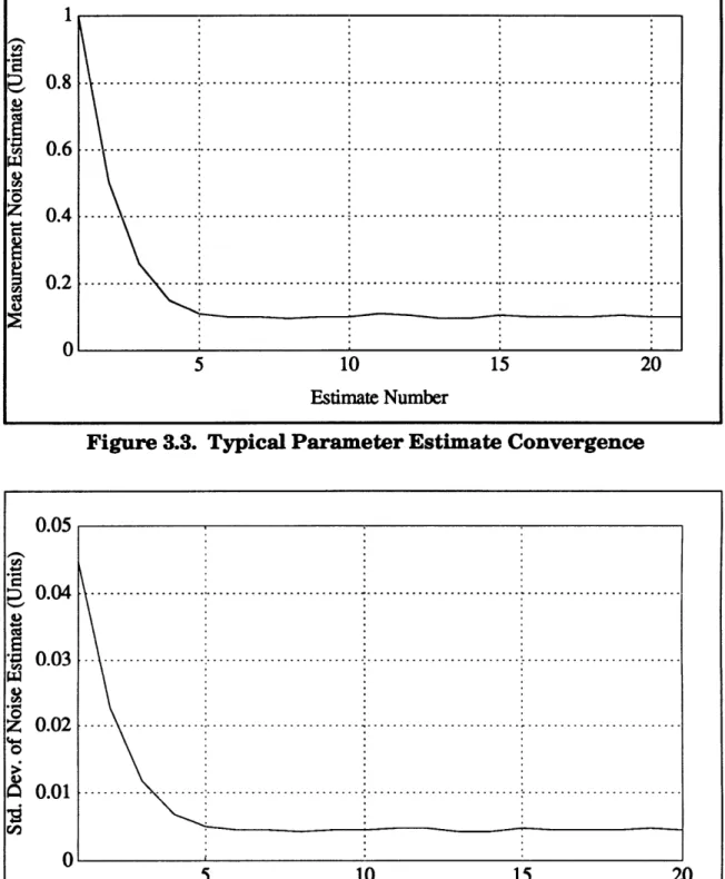
Figure 3.3. Typical Parameter Estimate Convergence... . 44

Figure 3.4. Typical Parameter Estimate Standard Deviation ... 44

Figure 3.5. Convergence of Measurement Noise Estimate... 45

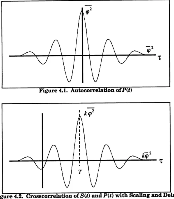
Figure 4.1. Autocorrelation of P(t) ... ... 49

Figure 4.2. Crosscorrelation of S(t) and P(t) with Scaling and Delay ... 49

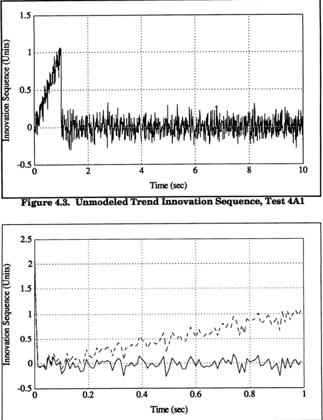
Figure 4.3. Unmodeled Trend Innovation Sequence, Test 4A1 ... 53

Figure 4.4. Modified Innovation Sequence, Test 4A1 ... 53

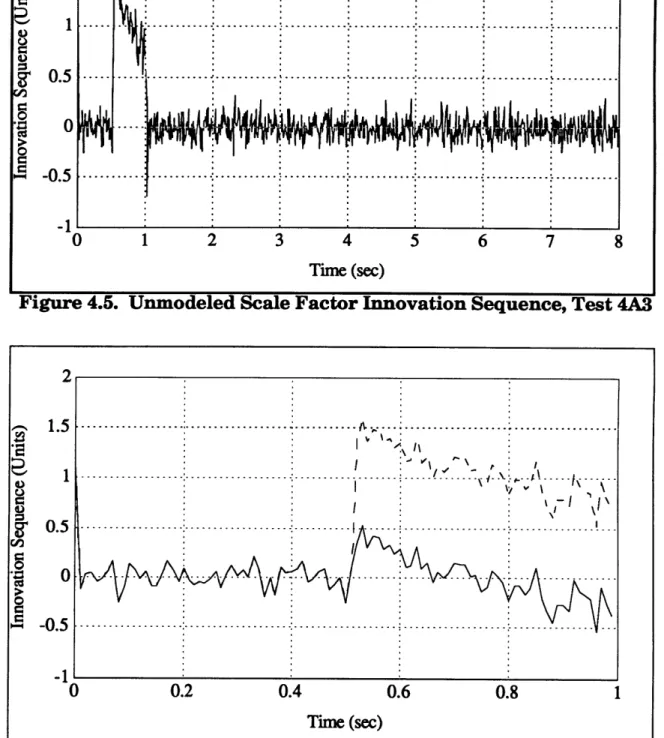
Figure 4.5. Unmodeled Scale Factor Innovation Sequence, Test 4A3 ... 54

Figure 4.6. Modified Innovation Sequence, Test 4A3 ... 54

Figure 4.7. Unmodeled Rate2 Term Innovation Sequence, Test 4A5... 55

Figure 4.8. Modified Innovation Sequence, Test 4A5 ... 55

Figure 4.9. Gas Bearing Gyro Output from Shaker Test, Test 4B ... 56

Figure 4.10. DIS System Model Innovation Sequence, Test 4B 1 ... 58

Figure 4.11. Model Adaptive Filter Innovation Sequence, Test 4B2 ... 58

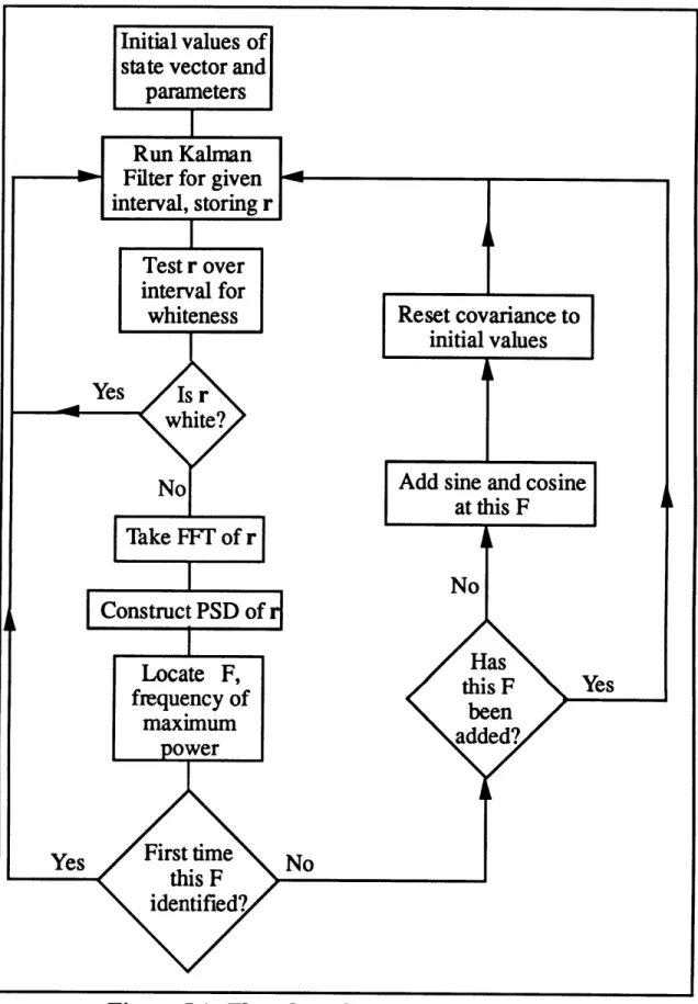
Figure 5.1. Flowchart for PSD Adaptive Filter... ... 66

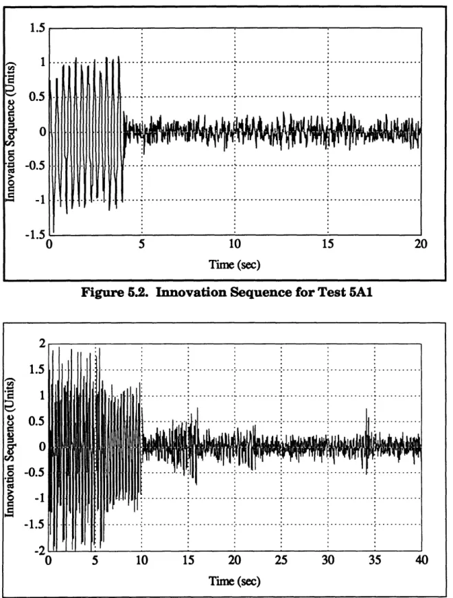
Figure 5.2. Innovation Sequence for Test 5A1 ... 69

Figure 5.3. Innovation Sequence for Test 5A3 ... 69

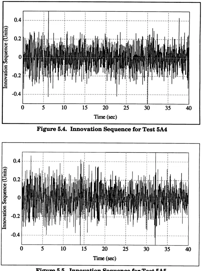
Figure 5.4. Innovation Sequence for Test 5A4 ... 70

Figure 5.5. Innovation Sequence for Test 5A5 ... 70

Figure 5.6. Probability of Detecting Frequency and Noise... 73

Figure 5.7. Aliased Frequency vs. Sampling Rate for 4400 Hz Signal ... 74

Figure 5.8. Probabilities for 2200 Hz Signal ... .... 75

Figure 5.9. Probabilities for 6600 Hz Signal ... 76

Figure 6.1. Innovation Sequence for Test 6A1 ... 81

Figure 6.2. Innovation Sequence for Test 6A2 ... 81

Figure 6.3. PSD of Original Raw Data for Test 6A2 ... 82

Figure 6.4. PSD of Innovation Sequence for Test 6A2 ... 82

Figure 7.1. Vibratory Micromechanical Gyroscope ... 94

Figure 7.3. Schematic of Tuning Fork Gyroscope ... .97

Figure 7.4. Tuning Fork Gyro Operation ... ... 98

Figure 8.1. Power Spectral Density for Test 8A ... ... 100

Figure 8.2. Standard Deviation vs. Bandwidth for Test 8A1 ... 100

Figure 8.3. Commanded Rate Profile for Test 8B ... ... 102

Figure 8.4. Inverted Gyro Output for Test 8B ... 103

Figure 8.5. Innovation Sequence of Kalman Filter for Test 8B 1 ... 104

Figure 8.6. Innovation Sequence of Adaptive Filter for Test 8B2... 104

Figure 8.7. Bias Estimate of Kalman Filter for Test 8B 1 ... 105

Figure 8.8. Bias Estimate of Adaptive Filter for Test 8B2 ... 105

Figure 8.9. PSD of Gyro Output for Stationary Drift Test, Test 8C ... 106

Figure 8.10. Standard Deviation vs. Bandwidth for Test 8C1 ... 107

Figure 8.11. Gyroscope Output for Test 8D ... 109

List of Tables

Table 3.1. Results of Maximum Likelihood Estimator Verification ... 43

Table 4.1. Results of Model Adaptive Filter Verification ... 51

Table 4.2. Model Adaptive Filter Analysis of Gas Bearing Gyro Data... 59

Table 5.1. Results of Periodic Noise Identification ... 68

Table 5.2. Probabilities for Aliased 4400 Hz Frequency Signal ... 73

Table 5.3. Probabilities for Aliased 2200 Hz Frequency Signal... 75

Table 5.4. Probabilities for Aliased 6600 Hz Frequency Signal ... 76

Table 6.1. Results of Raw Data Reduction Filter Verification ... 80

Table 6.2. Results of Reduced Data Analysis Filter Verification ... 87

Table 6.3. Kalman Filter versus Reduced Data Analysis Filter... 89

Table 8.1. Data Analysis on Stationary Drift Data, Test 8A2 ... 101

Table 8.2. Data Analysis on Stationary Drift Data, Test 8A3 ... 101

Table 8.3. Data Analysis on Stationary Drift Data, Test 8A4 ... 101

Table 8.4. Results for Commanded Rate Test, Test 8B ... 103

Table 8.5. Data Analysis on High Frequency Drift Data, Test 8C2 ... 108

Table 8.6. Data Analysis on High Frequency Drift Data, Test 8C3 ... 108

Table 8.7. Data Analysis on High Frequency Drift Data, Test 8C4 ... 108

Table 8.8. Results for Pressure Variation Test, Test 8D ... 110

Chapter 1

Introduction

1.1 Motivation

As newer inertial instrument technologies emerge, better data processing is needed for characterizing these instruments. These newer instruments are more sophisticated and their behavior challenges traditional data processing techniques. Traditional data processing has commonly used a triangular filter for reducing raw data and a Kalman filter for analyzing this reduced data according to a prescribed instrument model. These filters, however, can result in a less-than-optimum indication of instrument quality because both unmodeled error sources in the original signal, such as high frequency noise, and unknown factors in the instrument performance, such as temperature effects, are not accounted for in either aspect of the data processing. Because it gives more flexibility to data analysis, the need for adaptive filters has become significant. Instead of using fixed values, the adaptive filter seeks out the true values of the system so that both filter performance and instrument characterization are optimized.

Adaptive filter concepts can be used to develop filters for two aspects of data analysis. Raw data reduction is an important aspect of data processing. By decimating data, the computing time of the filter is reduced without sacrificing information on instrument performance. The traditional triangular filters create a weighted average of the raw data, but if noise in the signal can be eliminated before decimation of the data, then this analysis can be improved.

Analysis of this decimated data is crucial to determining instrument performance. To obtain optimal instrument performance, an adequate model of both the state vector and all noise sources is necessary. Often, though, the noise model is poorly understood, and unmodeled terms may exist in the system. A Kalman filter only analyzes the data with

respect to given parameters and a given state vector. With an adaptive filter, both the state vector and noise parameters can be adequately determined during data processing.

1.2 Adaptive Filter Concepts

In the next four chapters, adaptive Kalman filter concepts are developed and verified independently. First, the Kalman filter is reviewed. Next, a maximum likelihood estimator is developed. Correlation methods are then used to identify unmodeled state terms. Finally, power spectral density analysis is used to locate periodic noise sources.

1.2.1 Kalman Filter

Chapter 2 presents the Kalman filter. The innovation sequence (also known as the residual) is discussed, and its importance in adaptive filters is shown. In an optimal filter, the innovation sequence is a Gaussian white noise process. However, if the innovation sequence is not white noise, then information can be extracted from the sequence to optimize the filter. A white noise test procedure using correlation methods is presented. Some limits of the Kalman filter are discussed, including its inability to change parameters to reflect the data more accurately, and its inability to adapt the state model to achieve an optimal model.

1.2.2 Maximum Likelihood Estimator

In Chapter 3, maximum likelihood estimation of system parameters is presented. With this technique, unknown parameters in the Kalman filter matrices, such as the measurement noise standard deviation, can be estimated by maximizing the likelihood function of these parameters. By assuming that parameter values are slowly changing with respect to the state estimates, an online estimator is developed.

The maximum likelihood estimator was chosen for several reasons. It is capable of obtaining an unbiased efficient estimate, and it converges to the true values of the parameters as the number of samples grows without bound. This estimator is capable of

estimating the true values of both constant and slowly varying parameter values.

The scoring method is used for the maximum likelihood estimator, because this method has advantages over both a Newton-Raphson method and a conventional gradient method. The scoring method converges over a wider range than the Newton-Raphson method, and it converges more rapidly than a gradient method. The error in the scoring method is of order 1/N, where N is the number of samples. Verification of this approach is given with several analyses of simulated data.

1.23 Model Adaptive Filter

Chapter 4 discusses a model adaptive filter using correlation methods. By examining the relationship between the autocorrelation function of a random process, such as the instrument temperature, and the crosscorrelation function between that process and another random process, in this case the innovation sequence, a relationship between the two processes can be identified. A random process that is a function of another random process will have a crosscorrelation function that is equivalent to the autocorrelation function of the original signal, except for scaling and a time delay. If such a relationship does exist, the state vector of the Kalman filter is modified to account for this previously unmodeled term. The theory for this approach is derived, and verification of this filter using simulated data is shown. Real data is then used to show the effectiveness of the this filter in identifying a component of gyro drift error of an electromechanical gyroscope model due to g2 terms, DOS. This accomplishment is then placed in an historical context.

1.2.4 Periodic Signal Identification

Chapter 5 develops an approach for identifying unmodeled periodic signals in the innovation sequence. By using the Fast Fourier Transform, power spectral density analysis can identify any periodic signals in the innovation sequence. These unmodeled periodic signals can be included in the state model either as noise or as state terms; in both cases the filter performance will be improved. Although a periodic signal may be aliased, it can still be removed from the data. Once again, the theory behind this filter is given; verification of its effectiveness is demonstrated using simulated data for multiple frequency noise signals and also for variations in the frequency of the noise.

1.2.5 Data Analysis Filters

In Chapter 6, the three adaptive filter concepts are combined into two filters. The first adaptive filter, used for raw data reduction, is a combination of the maximum likelihood estimator and the PSD filter. By optimizing the filter parameters and by eliminating periodic noise, the best estimates of the data can be used for data decimation. Verification of the operation of this filter is given, and the performance of this filter is compared with that of a triangular filter for data decimation.

The second filter developed in Chapter 6 is a combination of all three adaptive filter concepts. This filter is used for reduced data analysis. By using all three techniques, the optimal estimates of the matrix parameters, as well as an accurate state model, can be

obtained. Verification of this filter is shown, and the improvements of this filter over a traditional Kalman filter are shown for simulated typical gyro outputs.

1.3 Data Analysis

After developing these two adaptive filters, micromechanical inertial instrument technology is discussed, and potential areas for the use of these filters are identified. Data files are then analyzed from several test runs, and improvements in instrument performance are shown.

1.3.1 Micromechanical Inertial Instruments

In Chapter 7, micromechanical inertial instrument technology is introduced, and micromechanical gyroscopes are briefly surveyed. The advantages and disadvantages of different gyroscope designs are presented. Also, the limitations and noise sources of these instruments are discussed, and possible solutions using adaptive filters are presented.

1.3.2 Data Analysis

In Chapter 8, adaptive filters are applied to outputs from various micromechanical gyroscopes. Comparisons between the adaptive filters and the traditional triangular and Kalman filter approach are made for all data analyzed. Various tests, including stationary drift tests and commanded rate tests, were run on different micromechanical gyroscopes, both the original micromechanical gyro design and the inverted gyro design. Improvements in data analysis were shown in both raw data reduction and reduced data analysis. The raw data reduction filter improvement ranged from 10 percent to 50 percent better than a triangular filter. The reduced data analysis filter is capable of reducing the RMS of the innovation sequence to half the RMS of the Kalman filter. A

pressure sensitivity and a rate squared sensitivity were identified by the adaptive filter.

1.3.3 Future Work

Chapter 9 presents the conclusions of this thesis, as well as some recommendations for future work. The algorithm used to compute the correlation functions can become computationally burdensome. A more efficient algorithm would increase online capabilities. This filter, if implemented on parallel processors, would easily be capable of real-time processing. By assigning the model adaptive and frequency location tests to secondary processors, the main processor could continue forward with data analysis, and the state model can be adjusted as necessary.

Chapter 2

Kalman Filter Theory

2.1 History of Estimators

The motivation to develop an effective estimator has existed for hundreds of years. In 1795, at the age of 18, Karl Friedrich Gauss developed the least squares method. His motivation was to find a method to determine the motion of the planets around the sun. In his work, Theoria Motus Corporum Coelestium, Gauss realized that single measurements were not accurate, but, by taking multiple measurements, the error of these measurements could be minimized. In the 1940s, Wiener and Kolmogorov both developed linear minimum mean-square estimators that spurred the development of the Kalman filter. Wiener developed an algorithm that minimized the mean-square error by choosing appropriate filter gains. Kalman then developed both the discrete and continuous versions of the Kalman filter in the early 1960s. The Kalman filter is basically a recursive solution to Gauss' original problem: the least squares estimator. Because of its computational efficiency and simplicity, the Kalman filter is an ideal choice for inertial instrument evaluation [45].

2.2 Kalman Filter Theory

A linear system can be expressed by the following stochastic difference equation,

x(ti+,) = 1(ti+lti )x(ti) + B(ti )u(ti)+ G(ti )w(ti) (2.1)

with available discrete-time measurements modeled by the linear relation,

z(ti)

=

H(ti )x(ti)

+

v(ti)

(2.2)

x = the state vector = n x 1 vector

= state transition matrix = n x n matrix u = deterministic input vector = r x 1 vector B = deterministic input matrix = n x r matrix G = system plant noise input matrix = n x q matrix z = the measurement vector = m x 1 vector

H = observability matrix = m x n matrix

ti = a discrete measurement time and,

w and v are independent, zero mean, white Gaussian noise processes with covariances

E{w(t i )w(t )T

}

E{v(ti)v(t )T} = R(ti )ij (2.4)

where Q is positive semidefinite and R is positive definite for all discrete time ti, E { ) is the expectation function, and Bij is the Kroneker delta. The initial conditions of the state vector are described by a Gaussian random vector with mean equal to Equation 2.5,

E{x(to)} = i(t ) (2.5)

and covariance equal to Equation 2.6,

E{[x(to) - i(to)][x(to) - (to )]T = P(to) (2.6)

The measurements, z, are processed to produce the state estimates, i. The state

transition equations are

i(t- ) = Q(t i, ti-1)i(tl I) + B(ti 1 )u(ti_) (2.7)

P(t- ) = (ti,ti-1 )P(t+_l )(t i,ti_1)T + G(ti-_l )Q(ti-_ )G(ti_ )T (2.8)

K(t) = [P(t )H(ti )T ]S(ti )-1 (2.9)

S(t

)

=

H(t

)P(t- )H(ti

+ R(ti)

(2.10)

The measurement incorporation equations introduce the new measurement into the state

ri = zi -H(t )i(t ) (2.11) i(t

(

i = the estimate of x based upon the most recent measurement

r = innovation sequence

S = covariance of innovation sequence and,

K = the Kalman gain matrix = n x m matrix.

The (+) and (-) superscripts on ti indicate whether the value at a particular ti is immediately before or immediately after the measurement incorporation at time ti. The notation (ti+l, ti) on 4 means that the matrix 4 is the transition between the state vector at sample times ti and ti+1. In these recursive equations, (D, H, B, and G may be time varying.

2.3 The Innovation Property of an Optimal Filter

In an optimal Kalman filter, the innovation sequence r (also known as the one step ahead predictor or residual shown in Equation 2.11) is a Gaussian white noise sequence with covariance S (Equation 2.10) [33, 34]. The innovation sequence is used to update i(t[~) by incorporating the information from the newest measurement, as shown in Equation 2.12. By proving that r is white noise in an optimal filter, this property of r can

then be used for filter optimization.

2.3.1 Innovation Sequence as White Noise in an Optimal Filter

First, define the error e(ti) as the difference between the true value of x(ti) and its estimate i(t,-):

e(t )= x(t

-

i(t)

(2.14)

This leads to a new definition of the innovation sequence,

ri

E{rir

}

= E(He(ti) + v(t))(He(t) + v(t ))T

E{rirT } = E{He(t

)(He(t

,)+

v(tj))T

= E{He(ti)(zj - Hi(ti ))T (2.17)

Also, the orthogonality principle [33] states that e(ti) is orthogonal to zk, for k < i. Since i(t) depends only on zk, for k <j, Equation 2.17 becomes

E{rir

=

A similar exercise shows that this is true for all i < j. For i = j,

E{r

R(ti)

This can also be proved by examining Equation 2.11. The measurement zi is a Gaussian random process, as is the state estimate i(t ). Therefore, the innovation sequence is also a Gaussian random process because it is a linear sum of Gaussian random variables. The innovation sequence is also a stationary process, as demonstrated by Mehra [33].

When the innovation sequence is white noise, then the filter is optimal. However, if the innovation sequence is not Gaussian white noise, then information required to optimize the filter can be extracted from the innovation sequence. For example, suppose a system is modeled with the following state vector

XZ

=X[

But the measurements fit the model,

zi=[1 1]X + v(ti) (2.21)

Because of the inadequate model for the state vector, the H matrix that is implemented in the Kalman filter is the 1 by 1 matrix [1], not the 1 by 2 matrix [1 1] that would be

expected from the measurement model. It is obvious that the state vector is an inadequate model for this measurement. This mismodeling will be stored in the innovation

sequence,

ri = z, - H(t i)i (t ) (2.11) which, in this example, becomes,

ri = x2(ti)+[Xl(ti)- A,(ti)]+ V(ti) (2.22)

In Equation 2.22, the difference term in xl is an unbiased Gaussian process. The innovation sequence r will contain the unmodeled term x2, and r will no longer be a Gaussian white noise sequence. However, the information needed to optimize the filter can be extracted from the innovation sequence. By adapting the matrices H and x to include the x2 term, the filter will be optimized.

2.3.2 White Noise Test for Optimality of Kalman Filter

A test is needed in order to exploit the innovation sequence for adaptive filtering. The white noise property of the innovation sequence in an optimal filter discussed in Section 2.3.1 will be used to develop an effective test. White noise has unique behavior for both the autocorrelation function and power spectral density analysis, as shown in Figure 2.1 [9]. Because a white noise process is independent, the autocorrelation sequence of white noise is an impulse at the zeroth lag term. Also, a white noise sequence is evenly distributed throughout the frequency domain, so that the power spectral density of white noise is a horizontal line. Either of these two properties of white noise could be used in a white noise test.

Autocorrelation Function Power Spectral Density Figure 2.1. Descriptions of White Noise Properties

The autocorrelation function was chosen for identification of the innovation sequence as white noise for two reasons. First, Mehra [33] shows that this function can be used to determine the whiteness of a sequence. Second, a test using the autocorrelation function

can be implemented easily. After calculating the autocorrelation function, confidence limits for this process can be established. The standard deviation of the measurement of autocorrelation is 1/ 4W, where N is the length of the innovation sequence. The confidence limits would be a given value times this standard deviation. For 95% confidence limits, the value is 1.96; for 99% confidence limits, the value is 2.58. Next, the number of points in the autocorrelation function that exceed these limits must be determined. If the percentage of points that exceed the confidence limits is greater than the confidence limit percentage, then the innovation sequence is not white noise. This test procedure is outlined in Equation 2.23 through Equation 2.25.

First, define Ck, the autocorrelation matrix of r, as shown in Equation 2.23.

Ck = E{rirTk (2.23)

A biased estimate of Ck may be obtained using Equation 2.24. For a scalar measurement, the estimate of Ck will be a scalar value. Mehra argues that the biased estimate should be used for this white noise test [33].

N

Ck = ri r i-k (2.24)

i=k

From this point, Mehra [33] shows that the test for optimality uses the normalized autocorrelation coefficients of the autocorrelation sequence, Pk. The normalized autocorrelation matrix can be estimated from Equation 2.25.

At IA 1 (2.25)

The diagonals of p k are compared with the confidence limits, and if the required percentage of the diagonal values are within this region, then the innovation sequence is white noise.

This test for optimality was implemented on MatlabTM _{for the Macintosh. The}

command xcorr calculates the normalized autocorrelation sequence [30, 42]. A comparison test is then run to determine the percentage of the sequence outside the 95% confidence limits.

2.4 Limitations of Kalman Filter

Although the Kalman filter is a very efficient estimator, it has certain limitations that arise when the state vector cannot be fully described. The Kalman filter works with a given state vector; if this description of the state vector is not adequate, then errors will result. These errors will affect the state estimates, because the filter cannot improve the state model on its own. For example, a trend error may exist in the data, but the Kalman filter cannot compensate for this term.

Also, the Kalman filter operates with fixed parameters. For example, the measurement noise covariance R is constant throughout data analysis. The Kalman filter then makes the best possible state estimates based on this R; if this value of R is wrong, then the Kalman filter estimates may not be optimal. These limitations of the Kalman filter are the driving forces in developing adaptive filters that are capable of compensating for unknown errors.

The following chapters will explore different methods of exploiting the information contained in the innovation sequence. The three methods used are maximum likelihood techniques, to enhance the estimates of the system parameters; correlation functions, to improve the state model; and power spectral density, to isolate periodic noise signals. Each of these methods seeks different information from the innovation sequence, and all three methods can be used simultaneously, as will be shown later.

Chapter 3

Maximum Likelihood Estimator

3.1 Motivation for Maximum Likelihood Estimator

Often, there is inadequate information about certain parameters in the Kalman filter matrices (D, B, G, Q, and R. For example, R, the measurement noise covariance matrix, may have uncertainty in its values. In order to obtain the optimal state estimates i, an accurate description of these parameter matrices is necessary. One way to do this is to use a priori statistical information in order to describe the parameter behavior for a particular system. However, it is usually not feasible to develop a probability density function model for the unknown variables, because the a priori estimates require previous information about the system. Therefore, another technique must be developed to determine these unknown parameters without previous data. The ideal approach would be able to adjust the unknown values based on the present data, and it would be able to do it with an efficient online method.

3.2 Maximum Likelihood Estimator

The maximum likelihood technique has been chosen for parameter estimation. This method will find an efficient estimate, if such an estimate exists. The efficient estimate is the unbiased (or at least negligibly biased) estimate with the lowest finite covariance of all unbiased estimates. Also, if an efficient estimate exists, the maximum likelihood estimator will have a unique solution that is equal to the efficient estimate. The maximum likelihood estimator is also consistent; it converges to the true value of the parameters as the number of sample elements grows without bound. This solution is both asymptotically Gaussian and asymptotically efficient. Also, given a single sufficient statistic for the estimated variable, the maximum likelihood estimate will be sufficient, and it will also be at least asymptotically efficient and unbiased [31].

To develop an online maximum likelihood estimator, an assumption is made that the parameters are essentially constant over a given interval of N sample periods, where N is arbitrary. This assumption can be implemented in one of two ways. At every sample time ti, the estimates can be based on the previous N measurements (tl, t2, t3, ... ), as

shown in Figure 3.1a. Or, at every N points, parameter estimates can be based on the previous N data points (tN, t2N, t3N, ... ), as shown in Figure 3.1b. However, in order to implement either maximum likelihood estimator, a likelihood function for the parameters must be chosen.

N

N

I

I

I

i

I

i

I

i-N

i

i+1

Figure 3.1a. Estimate Intervals at Every Sample Time

N

N

i-N

i

i+N

Figure 3.1b. Estimate Intervals at Every NSample Times

3.3 Maximum Likelihood Estimator Theory

For a given likelihood function L[O(t), i], where O(t) is the p length vector of variables (unknown parameters) and £ is the set of realized values of the measurements to be used as data, the objective of the maximum likelihood estimator is to find a value of O'(t,) that maximizes L[O(ti),fi] as a function of O(t,). This value can be found by solving Equation 3.1:

dL[ (ti

),fi

d (t)=

Peter S. Maybeck, in Chapter 10 of Stochastic Models, Estimation, and Control Volume 2, argues that the preferred likelihood function is [31]

which can also be expressed as

L = In fx(t),z,(t. Z(t,_N,a (4 , iiN+1 i-N, ,) (3.2a)

where,

x(ti) = state vector at time ti a = the parameter vector

Z(ti ) = _{measurement history z(tl), z(t2), z(t3}), ..., z(ti)

ZN(ti ) = _{most recent N measurements z(ti-N+1), z(ti-N+2), z(ti-N+3), ..., z(ti)}

Z(ti-N) = measurement history z(tl), z(t2), z(t3), ..., z(ti-N)

f = probability density function

This likelihood function exploits all a priori information and yields an effective and computationally feasible estimator. Equation 3.2a is similar to Equation 3.2, but it provides a fixed-length memory parameter estimator.

Applying Bayes' rule

fAlj

f Bjf

to Equation 3.2 yields the following relation of probability densities:

f₁ x(t z a = f1xt, Izt,),afz(t)fX

= fx(t )zi(t,),afz(t)Iz(t., ),afz(t_1 )ia

(3.4)

fx(t

iII

j=1

Each of these densities can then be written as

(2;))ll,

I(ti

exp{})

(3.5)

} = I- - x(t+ )j P(t, ) 4 - x(t+;)

where i(t+) and P(t+) are implicitly dependent upon the parameters (i.e. a) upon which the density is conditioned, and n is the length of i. Also, the probability densities in the product of Equation 3.4 are

(2 )= S(t

exp{.}

(2r)x _{S(t )1'}

(3.6)

where S(t;) is defined in Equation 2.1; i(t) P(t-), and S(t) are again implicitly dependent upon the parameters, and m is the length of the measurement vector z.

If Equations 3.5 and 3.6 are substituted into Equation 3.4, the likelihood function L then becomes

In

x(ti

zt,,).. (41E£,a)

n +im ln(2r)- In jP(

_'

_)'l

_1

2

±

j=1

where n and m are the lengths of the vectors x and z, respectively.

Inserting Equation 3.2 into Equation 3.1 yields the following pair of simultaneous equations:

= O _(3.8)

(3.9)

[n

f(,

.z,

£4

a) 4=x*(t) =

Substituting Equation 3.7 into Equation 3.8 leads to

4- )]T P(+ ) 4=x(ti) = OT ct=a 0 ) (3.10)

(j ini-'

(t;)]

fro ,).ze, a (,4 9f

{}= {- [j - H(tj

For which the solution is

x (ti) = (t0 )1a= (t)

Equation 3.11 demonstrates that the maximum likelihood estimate of the state vector is given by the Kalman filter equations when the unknown parameters are replaced by the best estimates of these parameters at time ti.

However, when Equation 3.7 is substituted into Equation 3.9, considerably more work is necessary to find a solution. The derivative of L with respect to the parameter a is given in Equation 3.12 [31].

-2

d

In

f(o

z(t),a

(R

£|

Ia)}

-

dad

S(t))

-[+ -

p(t

P(t:)-l [5 _

t(t)

=1 f

kt T

datr

(3.13)

-aj

- H(tja )(t(t

a

ak

)

(tk )-X[l

H(tj)i(tk)]

j=1 dGaa

Some important definitions of matrix differentiation that were needed for this problem are given in Equations 3.13 and 3.14.

dtnXll

_

dtnlXl dlXl_ 1 dlxl -

-1

dIXI

(3.13)

X- 1 ₌

_X-1 X - _(3.14)

da,

_dak

where X is a square matrix and ak is the kth component of a.

But, as shown in Equation 3.11, is equal to (tr+), so that the term 4- i(t~) is equal to 0. Also, for two vectors f and g, Frg = tr(fgT) = tr(gfT). Making these substitutions into Equation 3.12, the derivative of the likelihood function becomes

tr {P(t ). k

-

jl

H(tJ

)i(t)]

+ tr{[S(t)-1 - S(t)- [z - H(t )x(tj )][zj - H(tj )i(t )]T S(tj )-1

j=1

X dak at=a (ti ) (3.15)

The optimal solution for a solves this equation. However, there is no closed form solution to this problem; an iterative procedure must be used to find the optimal parameter vector, a*(t).

Using Equation 3.2a, a fixed-length memory parameter estimator can be developed with arguments similar to those shown in Equation 3.4. First, write the probability densities for the likelihood function,

fx(,ZN )IZ(ti-N ).a = fX(ti ZN (t ),z(ti-N),afZN(tA )IZ(ti-N ),a

fZN(ti)ti|N a

(ti z(ti),a ft (3.16)

fZ(ti-Nja

= fx(ti)jAz(ti).,

fz(t) z(t,_),a

j=i-N+1

In Equation 3.4, the lower limit on the product is 1. In Equation 3.16, the lower limit is i-N+1. Once again, the estimator yields the same state vector estimate as shown in Equation 3.11. However, in this case, the parameter equation is

tr

P(t)

d(t+

-2

da

H(tj

S(tj)-

rj

(3.17)

+

tr

[S(t)-'

-

S(tj)-1rr

]

,

)a=.*

j=i-N+1 I

where r is the innovation sequence defined in Equation 2.11 and S is the covariance of r.

3.4 Derivation of the Maximum Likelihood Kalman Filter

Using the ideas presented in the Section 3.3 and Chapter 2, a Kalman filter with maximum likelihood estimation of the parameters can now be developed [31]. The recursive formula for Equation 3.1 can be written using the Newton-Raphson method,

L[,(i),Zi -l dL[ ,(i),Zi]T

O

(ti)

= 0

(ti)

-

dt0

d

(3.18)

where 0*(ti) is the new estimate of the parameters at ti and .(ti) is the previous estimate of the parameters. The first derivative matrix in Equation 3.18 can also be

written as

L[O.

(ti

),Z

L[OZ, ]T

d

doO

and is called the gradient or score vector. The second derivative matrix is named the Hessian matrix, and it must be of full rank in order to be inverted. It is computationally

burdensome to use the Hessian, so the following approximation to the Hessian is used

d2L[* - J[ti (ti) _(3.20)

d02

In Equation 3.20, J is defined as

S0 L[,(t)]T

(ti)]

dL[Z(ti)]O

ill

,

dt,)

t

do

=

(ti)1

t A

_0*

_(ti)]

₌

_E

₁₀₌

_(ti)

_(3.22)

This approximation states that the second derivative matrix, the Hessian, for a particular realization of Zi , can be adequately represented by its ensemble average over all possible measurement time histories. With this approximation, only first order information about the likelihood function is required, and Equation 3.18 can then be expressed as

dL _{(t), Z(323)}

The scoring approximation, Maybeck argues, is a superior algorithm to both the Newton-Raphson method, which uses the Hessian matrix, and the conventional gradient algorithm [31]. With the conditional information matrix approximation, the error is of the order 1/N for large N. Also for large N, the rate of convergence approaches that of the Newton-Raphson method. Although scoring converges less rapidly near the solution than Newton-Raphson, it does converge over a larger region. The computational advantages over Newton-Raphson are also quite considerable. Scoring converges more rapidly than a gradient algorithm, but it requires slightly more computation to do so.

There are some problems with the scoring method, however. The initial J entries may be small, so that its inverse has large entries; this problem can be corrected by using a precomputed J value based on simulations or previous analysis. Also, J and J-1 must be constantly recomputed. However, after an initial transient, these values may be computed infrequently since J does not vary much after this transient has vanished. In this thesis, no problems with inverting J were encountered.

To generate parameter estimates, the score vector, (dL[i.(t),a.(t),Zi]/da)T_{, and the}

conditional information matrix J[ti,i.(t),A.(t)] must be computed. The score is equal to Equation 3.17 times -1, and the equation is evaluated with the actual estimate i.(t), not with the maximum likelihood estimate a' (t). The score is composed of the most recent N measurements. The score can be broken down into the sum of the N most recent single measurement scores, s [Z ,i.(t,)], and a final term y[Z,,i.(ti)]:

a

X(ti),'*(ti),Z,]= yk[Zi,*(ti)]+

A j=i-N+1

oak H()T S(tj)-lrj

(3.25a)

--

tr[S(t

)(t)

yk[Zi,a] =-

-1tr

P(t+)-1

dP(t

)}

The conditional information matrix can similarly be expressed in terms of a sum over the N most recent terms and a final term, if the parameter value is allowed to assume a

true, but unknown value, at:

Jk[ti,, (t ),at ]= E{ yk[Z(ti ),a]y[Z(ti),a]la = at

+

E

[Z(t

[Z(t),a]

a

= at

j=i-N+1

where

E{sk1 _{[Z(tj ),a]sll[Z(t ),a]la =}

_at)

S1

dtrS(t)

S(t)

dS(tj

=

S(t

)

S(t

d

a,

E{yk [Z(t),a]y[Z(ti),a]la = a

)

1

[PP(t)

)P(

=

2

dak;

a(t+

la =

d

a a

Equations 3.1 through 3.17 were derived without approximations. For Equations 3.18 through 3.27, the approximation has been made that the conditional information matrix J is equal to the Hessian; an approximation will also be made that these equations hold for values other than at.

3.5 Equations for Maximum Likelihood Kalman Filter

The maximum likelihood parameter estimator assumes that the parameters are constant over a period of N sample times [31]. At a sample time ti, the quantities at time

ti-N are unchangeable because nothing done in the present can affect a past estimate.

Therefore, the initial conditions of the N-step recursion for parameter estimation are:

X(tN )= previously computed (3.28a)

P(tN ) = previously computed (3.28b)

di(t-N ) = 0 _{(for all k) (3.28c)}

dak

P(t+-N)= 0 _{(for all k) (3.28d)}

dak

E

d

Ia

=

0

To solve for the parameter estimates, the score vector s1 and conditional information matrix J must be calculated. Both of these matrices depend on the derivatives of both the state vector and its covariance with respect to the parameter vector. In turn, these derivatives depend upon how the matrices of the system vary with the parameters. In order to determine this dependence, the derivatives of the Kalman filter equations are taken with respect to the parameter vector a. The Kalman filter is implemented as discussed in Chapter 2, but between each of the updates of the state vector, the derivatives of these vectors are also calculated. The procedure, then, for maximum likelihood estimation in a Kalman filter follows the flowchart in Figure 3.2. In this flowchart, the estimates of the parameters are made at every N points based on the previous N points, as shown in Figure 3.lb.

Initial values of

state vector and

parameters

Calculate Values

Incorporate

that are a function i

new estimates

of a given a. I

into matrices

i

Equations

Score Equations

for Time

Propagation

I

Conditional Information

Matrix Computations

for Time

Propagation

Measurement Incorporation

State Relations

Measurement Incorporation

Score Equations

Make new

parameter estimate s

Calculate

J and score vector

Calculate

y and E {Tyl }

Figure 3.2. Flowchart for Maximum Likelihood Estimation Before the filter can be implemented, certain values must be given. For example, the initial values of x and P, as well as the general form of the dependence of 4, B, Q, G and R on the parameter vector a, such as D/'Dak, R/~ak, etc., must be given. These matrices must be reevaluated for every new estimate of the parameters, I'(t). Once these functions of a are given, the following equations govern the filter.

No

Is

First, the state relation equations from Chapter 2 are processed using the most recent parameter estimate i'(t) to evaluate 0, B, Q, G and R as required:

f (tf ) = *(tp t-

+

)u(tj_

)

(2.7)

P(tJ )= 4(tj

)P(t_)(t ,tj_-

) +

G(tjl )Q(tj-

)G(tj-

(2.8)

K(tj) = [P(t )H(j )T ]S(tj )-1

(2.9)

S(t

)

=

H(tj )P(t7 )H(tj

+ R(tj )

(2.10)

The score equations for the time propagation are given by the p set of "sensitivity

system" equations. These equations, as well as all following equations, must be evaluated for k = 1, 2, ..., p, when the subscript k appears, (p is the length of the parameter vector a). First, the state vector estimate derivative is updated:

dr(t ) _ tj °(tf-1 ) °Q(tJt_ dB(tj_ )

a

'j-1

a

a

dak dak dak dak

Next, the derivative of the covariance matrix P is calculated:

dP(t

+G(t

)

t-1 ) G(tjl)T

+

Q(tj-)G(tj_

(3.30)

+ G ( t yj

)

Q

( t

dak

For the innovation sequence covariance matrix, S, the derivative update equation is:

aS (t,)

_(t

_H(tj)

P(t )

_P(t

_H(tj

)r aR(t )

_(3.31)

Also needed are the conditional information matrix computations for forward time

propagation (with time arguments tj-1 removed and a = i.(ti) reduced to a.). These

equations are used to solve E(sksl), and they are given in Equation 3.32 through 3.37. The expectation needed to calculate E(sksl) is shown in Equation 3.32.

adi

(tI) d.(ti

E

dak

da

.a

=

E

+

aj

A

dak daI

+(OE{

dax

= a(ti)

Ei++T

d

'

B

+

E{uuT'}

a

da,

d1

dBT

dak

daI

+4E

u adi*TIs}

dB'

+

_-a,

_dB

L

.T} a,

u ak

I

_.

Equation 3.32 requires the following expectations in order to be solved:

= QE{I+i+T A. QT +

BEuuT

I. }BT

+E{i+ul

}B + BE

ui+T

A

E ai

)

(tj

+E

dak

la

=

i.(ti)

=

I*

+d__

kJ

A

.}B

+

E{uu'TIa }BT

+o

_Eja T.B +B

Euif" a

ak

x}

ak

da

Ia

=

a (ti)}

--

_Ija

_laI

da,

E@(t- )-(t )

If u is precomputed, then E(u(T I .) can be written as uE(()T I .}) With this assumption, Equation 3.35 and Equation 3.36 can be evaluated and used to solve Equation 3.32 through Equation 3.34.

E(i(t

)I

}

=

Q(E( + a

+

Bu

(3.35)

And finally,

E a = D(t)

(ODE

I+

dak k k

k

where D(ti) is defined in Equation 3.38.

After these calculations are complete, E(skSl) can be solved with Equation 3.37.

E{sk

_{[Z(tj ),a]s'}

_{[Z(ty ), a]la}

₌

_{a, (t}

i

))

1 rS(j) S(tj ) S)- S(tj)

S2 )- t S(t)- _(3.37)

(t)

d

+2S(t)

H(tj

Next, the measurement incorporation state relations at time t are:

S= z - H(t )i(tj) (2.11)

D(tj)= I - K(tj )H(tj) (3.38)

i(tj) = i(t i)

)rj

(2.12)

P(tf) = [1

-

K(tj )H(tj )]P(t )

(2.13)

The measurement update score equations are then be processed using these definitions:

nj = S(tj )-1rj

(3.39)

C(tj)= S(tj)-' - njnT (3.40)

I

adi(t

)T

1

[Z

_{ig A*001}

2t

dak(C~f

)

dak

t

(3.41)

The second equation of the measurement update score equations can be developed by taking the derivative of Equation 2.10, as shown in Equation 3.42.

di(t)

dak

di(t

)

dK(tj)

dr

+

_{r + K(tj )}

)

dak

+ P(t- )H(tj

-dak

dr

dak

-H(tj)

Substituting Equations 3.43 and 3.44 into Equation 3.42 leads to the second measurement update score equation:

di(t+)

di(t

)

dP(t )

+

_,t,

i

[H(tj) nj]

A similar exercise with the derivative of Equation 2.13 gives the third measurement update score equation:

dP(tt )

dak

D(t)

P )

D(t)T

dak

dR(t. )

R(t)

K(tj)

) a,

The measurement update conditional information matrix equations are E E

da

i(t

da

la

A

= D(tj)E

di(tj

) di(tj )

T

dak

da

a

dP(tj

)

+D(tj)

_{ak H(t,}

₎

0K(tj )

dak

D(t )T

dP(t?)

S(tj )-1 H(tj)

) D(t)T