Learning a Markov Logic network for supervised gene regulatory network inference

The main objective of this research is to improve estimates of biomass by combining ALOS-2 SAR, Landsat 8, and field plots data in a tropical forest with high biomass values.. First,

Type C vessels - The database contains only two damage events for Type C vessels, both caused by the contact with MY ice.. Damage to Type D vessels was caused in ice regimes with

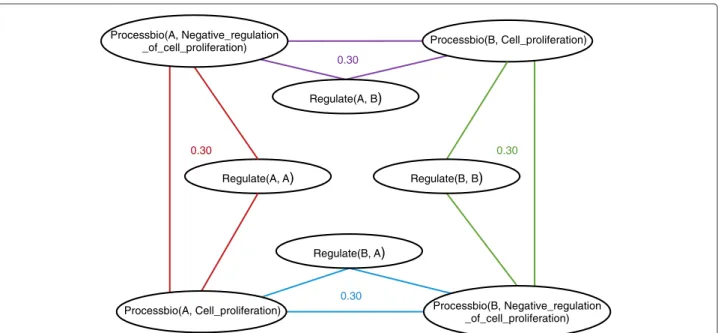
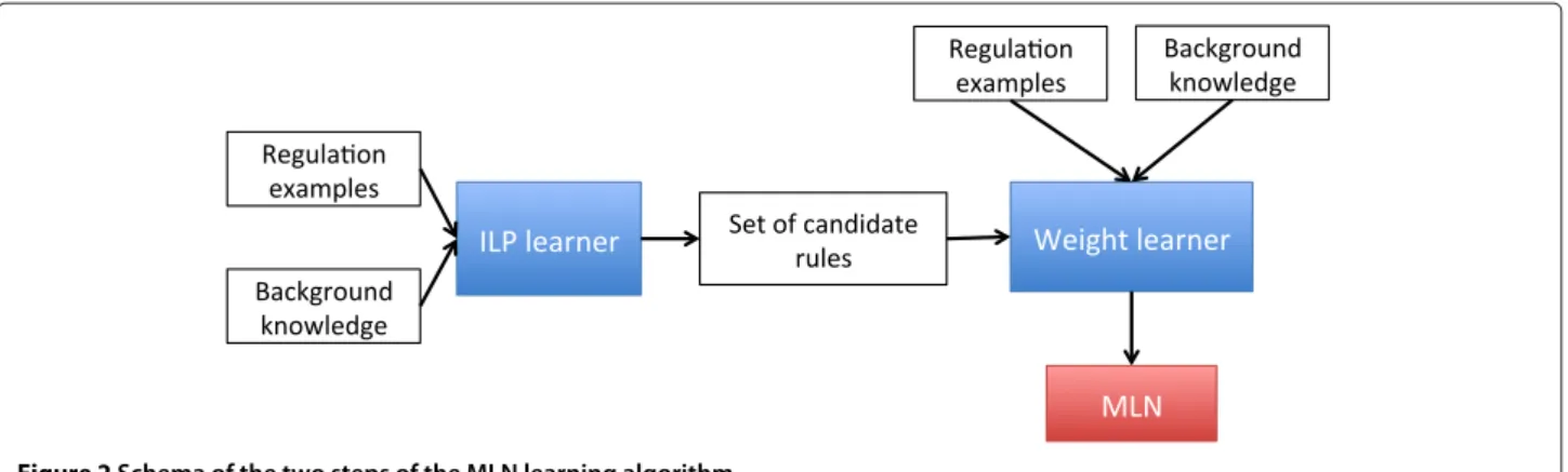
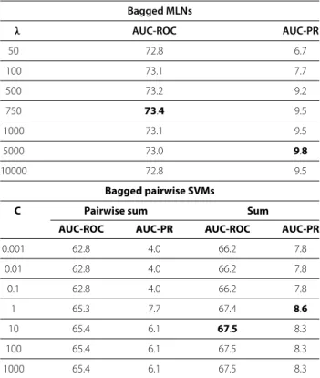
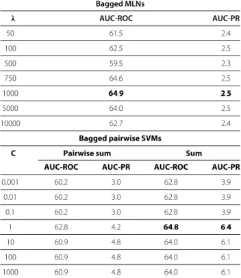
Despite the large number of available Gene Regulatory Network inference methods, the problem remains challenging: the underdetermination in the space of possible solutions

Durante i negoziati internazionali riguardanti il finan- ziamento dello sviluppo e l’agenda post-2015 sono emerse visioni assai diverse in merito alla responsa- bilità che i Paesi

• As we believe that floating-point on FPGA should exploit the flexibility of the target and therefore not be limited to IEEE single and double precision, the algorithm

/ La version de cette publication peut être l’une des suivantes : la version prépublication de l’auteur, la version acceptée du manuscrit ou la version de l’éditeur.. Access

L’objectif est ici d’apporter des éléments de réponse à la question du devenir des éléments traces dans un sol contaminé en comprenant mieux les interactions

The reactor performance was predicted to lie between the convection model where only the laminar flow profile is considered and the dispersion model which includes

References

1. Levine M, Davidson EH: Gene regulatory networks for development. PNAS2005, 102(14):4936–4942.
2. Lawrence N, Girolami M, Rattray M, Sanguinetti G (Eds): Learning and Inference in Computational Systems Biology, Cambridge: MIT Press; 2010. 3. Sima C, Hua J, Jung S: Inference of gene regulatory networks using
time-series data: a survey. Curr Genomics2009, 10(6):416–429. 4. Qian J, Lin J, Luscombe NM, Yu H, Gerstein M: Prediction of regulatory
networks: genome-wide identification of transcription factor targets from gene expression data. Bioinformatics2003, 19(15):1917–1926. 5. Mordelet F, Vert JP: SIRENE: supervised inference of regulatory
networks. Bioinformatics2008, 24(16):i76—i82.
6. Mordelet F, Vert JP: A bagging SVM to learn from positive and
unlabeled examples. ArXiv e-prints2010.
7. Cerulo L, Elkan C, Ceccarelli M: Learning gene regulatory networks
from only positive and unlabeled data. BMC Bioinformatics2010,
11:228.
8. Margolin A, Nemenman I, Basso K, Wiggins C, Stolovitzky G, Favera R, Califano A: ARACNE: an algorithm for the reconstruction of gene
regulatory networks in a mammalian cellular context. BMC
Bioinformatics2006, 7(Suppl 1):S7.
9. Faith JJ, Hayete B, Thaden JT, Mogno I, Wierzbowski, Cottarel G, Kasif S, Collins J, Gardner TS: Large-scale mapping and validation of
escherichia coli transcriptional regulation from a compendium of expression profiles. PLOS Biol2007, 5:e8.
10. Zoppoli P, Morganella S, Ceccarelli M: TimeDelay-ARACNE: reverse
engineering of gene networks from time-course data by an information theoretic approach. BMC Bioinformatics2010, 11:154. 11. Schafer J, Strimmer K: A shrinkage approach to large-scale covariance
matrix estimation and implications for functional genomics. Stat
Appl Genet Mol Biol2005, 4:Article 32.
12. de la Fuente A, Bing N, Hoeschele I, Mendes P: Discovery of meaningful
associations in genomic data using partial correlation coefficients.
Bioinformatics2004, 20(18):3565–3574.
13. Huynh-Thu VA, Irrthum A, Wehenkel L, Geurts P: Inferring regulatory
networks from expression data using tree-based methods. Plos ONE
2010, 5:e12776.
14. Friedman N, Linial M, Nachman I, Pe’er D: Using bayesian networks to
analyze expression data. J Comput Biol2000, 7:601–620. 15. Gardner TS, di Bernardo D, Lorenz D, Collins JJ: Inferring genetic
networks and identifying compound mode of action via expression profiling. Science2003, 301(5629):102–105.
16. Chen KC, Wang TY, Tseng HH, Huang CYF, Kao CY: A stochastic
differential equation model for quantifying transcriptional regulatory network in Saccharomyces cerevisiae. Bioinformatics2005,
21(12):2883–2890.
17. Bansal M, Gatta GD, di Bernardo D: Inference of gene regulatory
networks and compound mode of action from time course gene expression profiles. Bioinformatics2006, 22(7):815–822.
18. Yamanishi Y, Vert JP, Kanehisa M: Protein network inference from
multiple genomic data: a supervised approach. Bioinformatics2004,
20:i363—i370.
19. Kato T, Tsuda K, Asai K: Selective integration of multiple biological
data for supervised network inference. Bioinformatics2005,
21(10):2488–2495.
20. Ben-Hur A, Noble WS: Kernel methods for predicting protein-protein
interactions. Bioinformatics2005, 21(suppl 1):i38–i46.
21. Martin S, Roe D, Faulon JL: Predicting protein-protein interactions
using signature products. Bioinformatics2005, 21:218–226. 22. Hue M, Vert JP: On learning with kernels for unordered pairs. In
Proceedings of the 27th International Conference on Machine Learning; Haifa, Israel. Edited by Furnkranz J, Joachims T: Omnipress; 2010:463–470. 23. Bleakley K, Biau G, Vert JP: Supervised reconstruction of biological
networks with local models. Bioinformatics2007, 23(13):i57–i65. 24. Ceccarelli M, Cerulo L: Selection of negative examples in learning
gene regulatory networks.In Proceedings of the IEEE Interactional Conference on Bioinformatics and Biomedecine Workshop. Washington: IEEE Computer Society; 2009:56–61.
25. Cerulo L, Paduano V, Zoppoli P, Ceccarelli M: A negative selection
heuristic to predict new transcriptional targets. BMC Bioinformatics
2013, 14(Suppl 1):S3.
26. Elkan C, Noto K: Learning classifiers from only positive and unlabeled
data.In Proceedings of the 14th ACM SIGKDD International Conference on Knowledge Discovery and Data Mining, KDD ’08. Las Vegas, NV, USA. New York: ACM; 2008:213–220.
27. Giordana A, Saitta L: Phase transitions in relational learning. Mach Learn2000, 41(2):217–251.
28. Richardson M, Domingos P: Markov Logic: a unifying framework for
statistical relational learning.In Introduction to Statistical Relational Learning. Edited by Getoor L, Taskar B. Cambridge: the MIT Press; 2007:339–371.
29. Richardson M, Domingos P: Markov Logic networks. Mach Learn 2006,
62(1–2):107–136.
30. Kubat M, Matwin S: Addressing the Curse of Imbalanced Training
Sets: One-Sided Selection.In Proceedings of the 14th International Conference on Machine Learning; Nashville, Tennessee, USA. Edited by Douglas HF. San Francisco: Morgan Kaufmann; 1997:179–186.
31. Tao D, Tang X, Li X, Wu X: Asymmetric bagging and random subspace
for support vector machines-based relevance feedback in image retrieval. IEEE Trans Pattern Anal Mach Intell2006, 28(7):1088–1099.
(15)
32. Langlands K, Down GA, Kealey T: Id proteins are dynamically
expressed in normal epidermis and dysregulated in squamous cell carcinoma. Cancer Res2000, 60:5929–5933.
33. De Raedt L: Logical and Relational Learning. Berlin, Heidelberg: Springer; 2008.
34. Consortium TGO: Gene ontology: tool for the unification of biology. Nat Genet2000, 25:25–29.
35. Srinivasan A: The Aleph manual. 2007. http://www.comlab.ox.ac.uk/ activities/machinelearning/Aleph/aleph.html.
36. Muggleton S, De Raedt L: Inductive logic programming: theory and
methods. J Logic Program1994, 19(20):629–679.
37. Singla P, Domingos P: Discriminative training of Markov Logic
Networks.In Proceedings of the 20th national conference on Artificial intelligence - Volume 2; Pittsburgh. Menlo Park: The AAAI Press; 2005:868–873.
38. Lowd D, Domingos P: Efficient weight learning for Markov Logic
Networks.In Proceedings of the 11th European conference on Principles and Practice of Knowledge Discovery in Databases; Warsaw, Poland. Berlin Heidelberg: Springer; 2007:200–211.
39. Huynh T, Mooney R: Discriminative structure and parameter learning
for Markov Logic Networks.In Proceedings of the 25th International Conference on Machine Learning. Helsinki: Omnipress; 2008:416–423. 40. Huynh TN, Mooney RJ: Max-margin weight learning for Markov logic
networks.In Proceedings of the European Conference on Machine Learning and Knowledge Discovery in Databases: Part I, Bled, Slovenia. Berlin Heidelberg: Springer; 2009:564–579.
41. Liu DC, Nocedal J: On the limited memory BFGS method for large
scale optimization. Math Program1989, 45(3):503–528. 42. Kok S, Sumner M, Richardson M, Singla P, Poon H, Lowd D, Wang J,
Domingos P: The Alchemy system for statistical relational AI. Tech. rep., Department of Computer Science and Engineering, University of Washington, Seattle, WA; 2009. http://alchemy.cs.washington.edu. 43. Benjamini Y, Hochberg Y: Controlling the false discovery rate: a
practical and powerful approach to multiple testing. J R Stat Soc Ser B
(Methodol)1995, 57:289–300.
44. Li Y, Liu L, Bai X, Cai H, Ji W, Guo D, Zhu Y: Comparative study of
discretization methods of microarray data for inferring
transcriptional regulatory networks. BMC Bioinformatics2010, 11:520. 45. Aranda B, Achuthan P, Alam-Faruque Y, Armean I, Bridge1 A, Derow C, M Feuermann ATG, Kerrien S, Khadake J, Kerssemakers J, Leroy C, Menden M, Michaut M, L Montecchi-Palazzi S, Neuhauser N, Orchard S, Perreau V, Roechert B, van Eijk K, Hermjakob H: The IntAct molecular interaction
database in 2010. Nucleic Acids Res2010, 38(Database issue):525–531. 46. Maglott D, Ostell J, Pruitt KD, Tatusova T: Entrez Gene: gene-centered
information at NCBI. Nucleic Acids Res2011, 39(suppl 1):D52–D57. 47. Vert JP, Qiu J, Noble W: A new pairwise kernel for biological network
inference with support vector machines. BMC Bioinformatics2007,
8(Suppl 10):S8.
48. Kashima H, Kato T, Yamanishi Y, Sugiyama M, Tsuda K: Link propagation:
a fast semi-supervised learning algorithm for link prediction.In Proceedings of the 9th SIAM International Conference on Data Mining; Sparks, Nevada, USA: SIAM; 2009:1099–1110.
49. Kashima H, Oyama S, Yamanishi Y, Tsuda K: Cartesian kernel: an
efficient alternative to the pairwise kernel. IEICE Trans Inf Syst2010,
E93-D(10):2672–2679.
50. Davis J, Goadrich M: The relationship between precision-recall and
ROC curves.In Proceedings of the 23rd International Conference on Machine Learning, Pittsburgh. OmniPress; 2006:233–240.
51. DeLong ER, DeLong DM, Clarke-Pearson DL: Comparing the areas
under two or more correlated receiver operating characteristic curves: a nonparametric approach. Biometrics1988, 44(3):837–845. 52. Robin X, Turck N, Hainard A, Tiberti N, Lisacek F, Sanchez JC, Muller M:
pROC: an open-source package for R and S+ to analyze and compare ROC curves. BMC Bioinformatics2011, 12:77.
53. Lanckriet GRG, Deng M, Cristianini N, Jordan MI, Noble WS: Kernel-based
data fusion and its application to protein function prediction in yeast.In Proceedings of the Pacific Symposium on Biocomputing; Hawaii. Singapore: World Scientific; 2004:300–311.
54. Gönen M, Alpaydin E: Multiple kernel learning algorithms. J Mach Learn Res2011, 12:2211–2268.
55. Muggleton S, King RD, Stenberg MJ: Protein secondary structure
prediction using logic-based machine learning. Protein Eng1992,
5(7):647–657.
56. Kutsia T, Buchberger B: Predicate logic with sequence variables and
sequence function symbols.In MKM, Volume 3119 of Lecture Notes in Computer Science. Edited by Asperti A, Bancerek G, Trybulec A. Berlin Heidelberg: Springer-Verlag; 2004:205–219.
57. Niu F, Zhang C, Re C, Shavlik J: Scaling inference for Markov Logic via
dual decomposition.In Proceeding of the 12th IEEE International Conference on Data Mining (ICDM); Brussels, Belgium. Washington: IEEE Computer Society; 2012:1032–1037.
58. Blockeel H, Raedt LD: Top-down induction of first-order logical
decision trees. Artif Intell1998, 101(1-2):285–297.
59. Khosravi H, Schulte O, Hu J, Gao T: Learning compact Markov logic
networks with decision trees. Mach Learn2012, 89(3):257–277.
doi:10.1186/1471-2105-14-273
Cite this article as: Brouard et al.: Learning a Markov Logic network for supervised gene regulatory network inference. BMC Bioinformatics 2013 14:273.
Submit your next manuscript to BioMed Central and take full advantage of:
• Convenient online submission
• Thorough peer review
• No space constraints or color figure charges
• Immediate publication on acceptance
• Inclusion in PubMed, CAS, Scopus and Google Scholar
• Research which is freely available for redistribution
Submit your manuscript at www.biomedcentral.com/submit
Figure
Figure 1 Schema of a Markov network built from a MLN with C = { A , B }. The Markov network has been obtained from the clause (1) by considering a set of two constants A and B
Figure 2 Schema of the two steps of the MLN learning algorithm.