Université du Québec
Institut national de la recherche scientifique Centre Eau Terre Environnement
DEFINING A REFERENCE CLIMATE FOR CANADA THROUGH THE COMBINATION OF OBSERVATIONAL AND REANALYSIS DATASETS
Par Alexis Pérez Bello
Mémoire présenté pour l’obtention du grade de Maître es Sciences, M.Sc.
en sciences de l’eau
Jury d’évaluation
Examinateur externe Marie-Amélie Boucher Université de Sherbrooke Examinateur interne Sophie Duchesne
INRS, Centre Eau Terre Environnement Directeur de recherche Alain Mailhot
INRS, Centre Eau Terre Environnement
Acknowledgments
I want to thank all those people who in one way or another gave me their unconditional support in the realization of this work;
− To my family who have always given me all the necessary support and more.
− To my supervisor Alain Mailhot for the trust, his support, his right guidance, his patience (especially that) and for transmitting his experience in the process of developing this master project.
− To Guillaume Talbot for the constant and huge help from the first day I started. To Dikra Khedhaouiria for your help and advice.
− To all the members of the jury for agreeing to judge my work.
Sincerely, thank you very much
Résumé
Le présent travail propose une combinaison d’ensemble de différents jeux de données à l’aide de deux méthodes d’assimilation pour améliorer la qualité des champs de précipitation climatiques au Canada pour une période de 30 ans (1980-2009). Quatre ensembles de données de réanalyse ont été utilisés : CFSR, ERAI, JRA55 et MERRA. Les données d’observation proviennent de 2160 stations météorologiques à travers le pays avec un minimum de 10 années valides de précipitations quotidiennes. De plus, les données d’observation sur grille de Ressources Naturelles Canada (NRCan pour Natural Resources Canada) ont été utilisées à fin de comparaison. Les Indices de Précipitation Climatiques (IPC) ont été calculés pour chaque ensemble de données annuellement et ont été combinés (la Réanalyse + les Observations) par les méthodes d’Interpolation Optimale (OI pour Optimal Interpolation) et d’Interpolation Optimale d’Ensemble (EnOI pour Ensemble Optimal Interpolation) respectivement. Une vérification a été effectuée sur les stations qui ont été utilisées pour la combinaison, de même qu’une stratégie de validation croisée. Les résultats ont montré des améliorations au niveau des nouveaux ensembles de données de référence créés par les deux méthodes, en particulier pour l’approche d’ensemble. L’ensemble de données sur grille développé (par EnOI) a surpassé NRCan, lequel a été généré seulement à partir d’observations, ce qui montre que ce dernier devrait être utilisé avec précaution pour l’analyse d’événements de précipitation extrême. L’ensemble de données produit pourrait être utilisé pour les études d’impact de changement climatique et de stratégies d’adaptation de même que pour fournir une meilleure compréhension du climat actuel au Canada.
Mots-clés Interpolation optimale d’ensemble, Indices de Précipitations Climatiques, Assimilation de Données
Abstract
The present work shows a combination of different datasets through two data assimilation methods in order to improve the quality of the climate precipitation fields in Canada for a period of 30 years (1980-2009). Four reanalysis datasets were used; CFSR, ERAI, JRA55 and MERRA. The observational dataset consists in 2160 meteorological stations across the country with a minimum of 10 valid years of precipitation records available. Besides, the Natural Resources Canada gridded dataset (NRCan) was also used. The Climate Precipitation Indices were calculated for each dataset annually and were combined (Reanalysis + Observations) by the Optimal Interpolation (OI) and Ensemble Optimal Interpolation (EnOI) methods respectively. The verification was carried out over the stations that were used in the combination, but also through a cross-validation strategy. Results show the improvements in the new reference datasets created by both methods highlighting the Ensemble approach as the best. The reference gridded dataset developed (by EnOI) outperformed NRCan which was created only by observations and showing that the latter should be used with caution for extreme precipitation events analysis. The dataset produced contributes to the development of climate change impact studies and adaptation strategies, as well as providing a better understanding of the current climate in Canada.
Keywords Ensemble Optimal Interpolation, Climate Precipitations Indices, Data Assimilation
Contents
Acknowledgments iii Résumé v Abstract vii Contents ix List of Figures xiList of Tables xiii
List of abbreviations xv
I Synthesis 1
1 Introduction 3
2 Basic notions 5
2.1 Extreme precipitation events and indices . . . 5
2.2 Reanalysis . . . 6
2.3 Optimal Interpolation and Ensemble Optimal Interpolation . . . 7
3 Methodology 9 3.1 Datasets used . . . 9
3.2 Climate Precipitation Indices . . . 11
3.3 Workflow diagrams . . . 11
3.4 Validation procedure . . . 12
4 Results and discussion 15 5 Summary and Conclusions 21 II Article 23 1 Defining a reference climate for Canada through the combination of observational and reanalysis datasets 25 1.1 Abstract . . . 26
1.2 Introduction . . . 27
1.3 Datasets . . . 29
1.4 Climate Precipitation Indices and Super-Observations . . . 31
1.5 Optimal Interpolation (OI) . . . 34
1.6 Ensemble Optimal Interpolation (EnOI) . . . 36
1.7 Cross-validation procedure . . . 37
1.8 Results and Discussion . . . 40
1.8.1 Comparison of reanalysis, OI, and EnOI datasets . . . 40
1.8.2 Cross-validation . . . 42
1.8.3 Comparison of EnOI and NRCan gridded interpolated datasets . . . 46
1.9 Summary and conclusions . . . 50
References 53
List of Figures
3.1 Creation of super-observations. Panel on left shows the original stations network while the panel on right-hand side shows the corresponding network of super-observations. . . 10 3.2 Example of the grids for the various reanalysis, blue lines: CFSR; green lines: ERAI;
dashed red lines: JRA55; magenta lines: MERRA. . . 11 3.3 Workflow diagram for OI method . . . 12 3.4 Workflow diagram for EnOI method . . . 12 4.1 Violin and box plots showing the NE (averaged over all ten indices) after the
application of the data assimilation techniques. Boxes represent inter-quartiles range (first, Q1 and third, Q3), line inside the box the median value and outliers correspond to the black dots. Outliers are defined as values 1.5 times the interquartile distance (IQR=Q3-Q1) (whiskers) above or below Q3 or Q1 respectively. . . 16 4.2 Annual values of V (see equation 4.1) after applying OI to each reanalysis (top
12 rows) and after applying EnOI (bottom four rows) averaged over all CPI for the various cross-validation subnetworks (Near and Far configurations with 10, 30 and 50% validation sites). Black dots correspond to the datasets with the largest improvements for a given cross-validation subnetwork. . . 17 4.3 Violin plots showing the bias between EnOI or NRCan and observed values at all
the stations for PRmean, PR1mm, RX1day, RX5day, R10mm and R20mm. Boxes represent inter-quartiles range (first, Q1 and third, Q3), line inside the box the median value and outliers correspond to the black dots. Outliers are defined as values 1.5 times the interquartile distance (IQR=Q3-Q1) (whiskers) above or below Q3 or Q1 respectively. . . 18 4.4 Violin plots showing the bias between EnOI or NRCan and observed values at all the
stations for CDD, CWD, SDII and PRCPTOT. Boxes represent inter-quartiles range (first, Q1 and third, Q3), line inside the box the median value and outliers correspond to the black dots. Outliers are defined as values 1.5 times the interquartile distance (IQR=Q3-Q1) (whiskers) above or below Q3 or Q1 respectively. . . 19 1.1 Map of the stations considered in this study. . . 31 1.2 Number and percent (above each bar) of stations with given numbers of valid years. 31 1.3 Total number of stations and super-observations available each year. . . 33 1.4 Estimated correlation function (continuous curve) with corresponding discrete values
for the RX1day from CFSR. . . 35 1.5 Spatial distribution of calibration (red) and validation (blue) sites on year 1980 for
(a) Near and (b) Far subnetworks with 10% validations stations. . . . 39
1.6 Violin and box plots showing the distances between all validation sites and their closest calibration sites for Near and Far subnetworks respectively over the study period. Boxes represent inter-quartiles range (first quartile Q1 and third quartile Q3), line inside the box the median value and outliers correspond to the black dots. Outliers are defined as values 1.5 times the interquartile distance (IQR=Q3-Q1) (whiskers) above or below Q3 or Q1 respectively. . . 39 1.7 Taylor diagrams comparing the observed and estimated annual CPI values over the
1980-2010 period at all station sites: a) before applying OI; b) after applying OI; c) after applying EnOI. . . 41 1.8 Annual NRMSD (averaged over all stations and all CPI) values normalized by the
observational standard deviation (σ over all valid stations for a given year) for each reanalysis after applying OI and EnOI. . . 42 1.9 (a) Distance between each grid point and the closest station and (b) expected relative
CPI error (equation 1.7) as a function of the distance to closest station. . . 43 1.10 Mean Absolute Error of the analysis field (M AEA) normalized by the Mean Absolute
Error of the background field (M AEB) over all validation sites for the entire period (1980-2009) (equation 1.14) and each CPI (x-axis). Near (N) and Far (F) configurations with 10, 30, and 50% validation points after applying OI to the four reanalyses (top four rows) and after applying EnOI (bottom row) are presented. Black dots identify, for each CPI, the datasets with the lowest V1 values for a given
subnetwork (N or F with 10, 30, or 50% of validation points). . . 45 1.11 RMSD of the analysis field (RM SDA) normalized by the standard deviation for each
CPI (σB) of annual values at all validation sites for the entire period (1980-2009)
(equation 1.15) and each CPI (x-axis). Near (N) and Far (F) configurations with 10, 30 and 50% of validation points after applying OI to the four reanalyses (top four rows) and after applying EnOI (bottom row) are presented. Black dots identify the datasets with the best performance (smallest values) for a given subnetwork (N or F with 10, 30, or 50% validation points) and CPI. . . 46 1.12 Mean PRmean (first line), PR1mm (second line), and RX1day (third line) values
over the 1980-2009 period as estimated from the EnOI (left column), NRCan datasets (middle column), and corresponding grid-to-grid differences between EnOI and NRCan (right column). . . 47 1.13 Scatter plots of PRmean (first line), PR1mm (second line), and RX1day (third line)
values estimated from EnOI (left column) and NRCan (right column) dataset against the corresponding observed values. . . 48 1.14 Taylor diagram comparing annual CPI values at station sites estimated with NRCan
gridded dataset (red symbols) and after applying EnOI (blue symbols). . . 49
List of Tables
1.1 Gridded datasets used in this study (acronyms appearing in parenthesis are used to refer to these datasets). . . 30 1.2 Climate Precipitation Indices, adapted from Zhang et al. (2011) . . . . 32
List of abbreviations
AHCCD Adjusted and Homogenized Canadian Climate Data
ANUSPLIN Program for interpolating data using a thin plate spline smoothing algorithms CFSR Climate Forecast System Reanalysis
CMIP5 Coupled Model Intercomparison Project Phase 5 CPI Climate Precipitation Indices
EnKF Ensemble Kalman Filter
EnOI Ensemble Optimal Interpolation ERAI ERA-Interim Reanalysis
ETCCDI Expert Team on Climate Change Detection and Indices IPCC Intergovernmental Panel on Climate Change
JRA55 Japanese 55-year Reanalysis MAE Mean Absolute Error
MDDELCC Ministère du Développement Durable, de l’Environnement et de la Lutte contre les Changements Climatiques
MERRA Modern-Era Retrospective Analysis for Research and Applications NE Normalized Error
NRCan Natural Resources Canada (observational gridded dataset) NRMSD Normalized Root Mean Square Difference
NSD Normalized Standard Deviation OI Optimal Interpolation
RMSD Root Mean Square Difference
Part I
Chapter 1
Introduction
During the last decades, many major precipitation events have been reported in many parts of the world (Hartmann et al., 2013). These events are expected to be more frequent and intense over the course of the 21st century due to climate change (Stocker et al., 2013). It is therefore important to assess how these types of events will evolve in a future climate in order to better assess their potential impacts on ecosystems, economy and the societies as a whole and to develop adequate adaptation strategies.
Defining and characterizing the historical climate is crucial to assess the projected future changes (Hatzaki et al., 2010). Reference climate can be defined and characterized in many ways. The Expert Team on Climate Change Detection and Indices (ETCCDI) proposed a set of annual precipitation indices that can be estimated from daily precipitation series (Peterson et al., 2001; Zhang et al., 2011) (Climate Precipitation Indices, hereafter CPI). Spatial distribution of such indices over a given region requires a dense network of meteorological observations and historical climate can be readily defined in regions where a large meteorological network has been deployed over the recent decades (Heim, 2015). However, this remains a huge challenge for regions with sparse network or with short records. In such cases, other datasets must be considered. Despite the existence of these alternative datasets, it must be reminded that records from meteorological stations remain the primary and possibly the most reliable source of data for historical climate. The lack of a dense network of observations with long time records, especially in the northern parts of Canada, therefore represents a huge challenge (Wang et al., 2017).
4
Reanalyses are an interesting alternative source of information for different climate applications. They provide consistent gridded datasets in space and time that could be useful for regions with sparse network or short records. Despite improvements in the spatio-temporal representation of many variables brought by reanalysis, precipitation remains a problematic field because observations of this variable have not been explicitly used to create most of the available reanalyses (Zwiers et al., 2013). However, Diaconescu et al. (2017) showed that reanalyses should be used with caution for the northern parts of Canada. Therefore, reanalyses need to be bias corrected before they can be used as a reference dataset. One possible option for improving the CPI representation is through the combination of reanalysis datasets with in situ observations through data assimilation methods. The aim of this study is to improve the quality of the annual climate precipitation fields for Canada over the period 1980-2009. It is based on the hypothesis that it can be done by combining annual CPI from surface weather stations with reanalyses through data assimilation techniques. In order to merge both datasets, Optimal Interpolation (hereafter, OI) and Ensemble Optimal Interpolation (hereafter, EnOI) methods were used. This document is divided in two parts. The first part (“Synthesis”) is a summarized description of the study as well as complementary information (Basic notions, Methodology, Results, Conclusions) that provides details about the different steps used in this study. The second part is a scientific paper ready for submission.
Chapter 2
Basic notions
2.1
Extreme precipitation events and indices
The Intergovernmental Panel on Climate Change (IPCC), Special Report on Managing the Risks of Extreme Events and Disasters to Advance Climate Change Adaptation (Seneviratne et al., 2012) defines an extreme climate event or an extreme weather event as “the occurrence of a value of a weather or climate variable above (or below) a threshold value near the upper (or lower) ends of the range of observed values of the variable”. For precipitation values, this definition basically refers to events located in the tails of the probability distributions with low frequency of occurrence. Extreme events can also be analyzed in many different ways depending on applications (Zwiers et al., 2013). For instance, for low frequency of occurrence (more than a year), different methods based on extreme value theory (Coles, 2001) can be used. Those methods are based on statistical models designed to estimate the probability of occurrence of such events over a period beyond the recorded one (Zhang & Zwiers, 2013). Some examples of application of those methods for extreme precipitation events are presented in (Kharin et al., 2007; DeGaetano, 2009; Mishra & Singh, 2010; Rajczak et al., 2013; Rahimpour et al., 2016; Santos et al., 2016).
The Expert Team on Climate Change Detection and Indices (ETCCDI) proposed a set of indices to characterize extreme precipitation and temperature (only precipitation indices are considered hereafter). A majority of these indices aim at characterizing events that occur at least once a year and are called “moderate extremes” (Zhang et al., 2011). These indices can be divided in three
6
groups depending of their characteristics. The first group includes indices that are absolute values of the variable analyzed. The Annual maximum of daily precipitation (RX1day) as well as the annual maximum precipitation over 5 consecutive days (RX5day) belong to this group. These indices can be used to estimate annual maximum values of different return periods. The second group includes indices that meet a given condition, defined by a fixed threshold, counting the number of days when this condition is met. Example of such indices are the number of days with precipitation values with more than 10, 20 or 30 mm (R10mm, R20mm, R30mm) and the number of wet days (days with precipitation values above 1 mm, PR1mm). This group also includes indices related to persistence of given meteorological conditions such as the annual maximum number of consecutive dry days (when precipitation is below 1 mm, CDD) and the annual maximum number of consecutive wet days (when precipitation is above 1 mm, CWD). The third group includes indices that refer to extreme quantiles of the index distribution over a specified climatological period. An example of such index is the annual number of days with daily precipitation above the 95th percentile of precipitation distribution defined over a specific reference period. This third group of indices were not considered in this study.
Extreme precipitation indices have been used to characterize changes in frequency and intensity in different regions around the world. Five precipitation indices over the period 1946-1999 were analyzed by Frich et al. (2002), and global maps representing multi-decadal changes at observational sites were created. In that study, despite Africa and South America were not considered, resulting analysis showed significant increases in climate extremes. A comprehensive and updated global gridded land-based representation of extreme precipitation indices was presented by Alexander et al. (2006) using eleven indices for the period 1951-2003, and later by Donat et al. (2013), using 12 indices over the period 1901-2010. In both studies, detected trends indicated an increase toward wetter conditions in many regions of the globe.
2.2
Reanalysis
Over the last decades, reanalyses have been increasingly useful for many climate applications. A considerable amount of research has been realized using these datasets. Reanalyses are created from the combination of a numerical model and different sources of observational datasets through a data assimilation routine (Bosilovich et al., 2008). They provide a consistent and comprehensive
Chapter 2. Basic notions 7
three dimensional grid representation of the main atmospheric variables throughout the world (Dee et al., 2011). Their quality have been improved recently due to the progress reached in data assimilation methods, the rescue of past observations as well as the homogeneous products obtained from satellites (Kobayashi et al., 2015). Their performance depends of different factors, like: the data assimilation technique, the variable considered for the analysis, the sources of observations used, as well as the forecast model (Lorenz & Kunstmann, 2012). As these factors have been continuously improving over the last years, it is evident that many reanalyses should be considered for specific applications (Saha et al., 2010). The extreme precipitation indices derived from reanalyses have been used in different studies. Sillmann et al. (2013) used four reanalysis data sets to assess the performance of Coupled Model Intercomparison Project Phase 5 (CMIP5) models using 11 precipitation indices. Reanalyses were also compared to global gridded observational datasets by Donat et al. (2014) using 2 precipitation indices. These authors showed the spatial distribution of precipitation as simulated by reanalyses improved in the satellite era. For the northern parts of Canada, Diaconescu et al. (2017), considering 10 precipitations indices, showed that reanalyses should be used with caution over these regions for precipitations related indices. It is important also to note that precipitation is a direct output of numerical models and that ground precipitation records are not assimilated (Kalnay et al., 1996).
2.3
Optimal Interpolation and Ensemble Optimal Interpolation
The OI method (Kalnay, 2002), also known as statistical interpolation (Daley, 1991), combines the information from two datasets (e.g. simulated and observed datasets) by exploiting the horizontal correlation distribution between these datasets. The resulting field is expected to be a better representation of the real conditions. EnOI (Evensen, 2003) is an approximation of the Ensemble Kalman Filter (EnKF) in which an ensemble of model states in long time integration (stationary) is used to compute the analysis field (field obtained after the merging process) and only one model state is used as background field (initial field before the merging process) (Oke et al., 2006). Both methods solve the same analysis equation and differ only in how the (background or model) error covariance is defined (Ren & Hartnett, 2017). While for OI it can be created depending on the distance between the stations and can be represented as a continuous function (e.g. such functions can be found in Buell (1972)), for EnOI an ensemble of model states is needed.
8
OI method has been used to merge different sources of precipitation datasets. A system for mesoscale analyses in the north of Europe was developed by Häggmark et al. (2000) where different sources of observations (e.g. satellites, radars and automatic stations) were used. Over Canada, a preliminary real-time precipitation analysis at 15 km of spatial resolution and 6 hours of precipitation accumulation is described in Mahfouf et al. (2007). An evaluation of this dataset was later provided by Lespinas et al. (2015) and the assimilation of precipitation estimations obtained from radars were added by Fortin et al. (2015). For climatological purposes, a 5.5 km grid spacing precipitation reanalysis over Europe was created by Soci et al. (2016). Furthermore, for global scale, satellites information, surface observations and models were combined with significant improvements also at regional scales (Nie et al., 2016).
These methods have been also used to assimilate or combine other variables from the ocean-atmosphere system. Some examples in ocean data assimilation can be found in (Kimoto et al., 1997; Oke et al., 2010; Fu et al., 2011; Ratheesh et al., 2014; Ji et al., 2015; Mignac et al., 2015). They have been also applied to assimilate some wave parameters improving the quality of the forecasts, (Qi & Cao, 2015; Cao et al., 2015; Rusu & Guedes Soares, 2016). Furthermore, for air quality analysis (Candiani et al., 2013; Tang et al., 2015) and for daily streamflow (retrospective estimation) in ungauged rivers by Lachance-Cloutier et al. (2017). These widely used methods were used in this work to combine reanalysis datasets with surface weather stations over Canada.
Chapter 3
Methodology
This chapter intends to provide complementary information to help understand the different steps of the methodology used in this study. The main steps are presented in the paper (See Article 1).
3.1
Datasets used
Figure 1.1 of the paper presents a map of the ground weather stations used in this study. Daily precipitation records from the Adjusted and Homogenized Canadian Climate Data (AHCCD) developed by Environment Canada and from the stations operated by Ministère du Développement Durable, de l’Environnement et de la Lutte contre les Changements Climatiques (MDDELCC) from Quebec were used. Only stations with available records during the period 1980-2009 were considered. As can be seen, stations unevenly cover the territory and are mainly concentrated in the southern part of the country. Another important limitation is the significant number of missing values in the available records (Figure 1.2). Table 1.1 of the paper provides a summary of the characteristics of the gridded datasets used in this study. Those are divided into two groups. The first group comprises four reanalyses (CFSR, ERAI, JRA55, and MERRA) and the second group includes the NRCan observational gridded dataset. It is important to mention that not all the stations considered in this study were used to create the NRCan dataset (for instance, some stations operated by the MDDELCC in Quebec were not used). This dataset is available for the whole territory of Canada and it is easily accessible. In order to compare reanalysis grid points
10
(interpreted as average values over a grid cells) and stations (at-site value), super-observations or upscaled observations (Cherubini et al., 2002) were defined for grid cells containing many stations. Figure 3.1 shows a graphical representation of how super-observations were created and Equation 1.1 of the paper shows how their values were estimated. Reanalysis grid points (in this case CFSR) are represented by the black dots and the dashed lines define the grid cells, red dots represent the stations while super-observations are represented by green dots (position of super-observations are determined by the weighted centroid of stations positions; the position of super-observations for grid cells with one station are superimposed to station position). Figure 1.3 of the article shows the number of observations per year over the study period as well as the number of super-observations, the latter were chosen to combine with reanalysis by OI and EnOI methods respectively.
Figure 3.1 – Creation of super-observations. Panel on left shows the original stations network while the panel on right-hand side shows the corresponding network of super-observations.
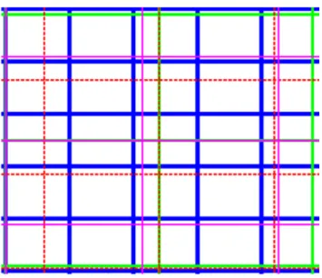
Table 1.1 of the paper shows that reanalysis grids have different spatial resolution. Figure 3.2 presents an example of each of these grids.
In order to apply the EnOI method which combines the information from the four reanalyses, a common grid must be defined. The grid of the reanalysis with the finest resolution, CFSR, was selected. Once CPI values are estimated from each reanalysis on their respective native grid, a conservative remapping procedure (Jones, 1999) was used to match CPI values from each native grid to the reference grid.
Chapter 3. Methodology 11
Figure 3.2 – Example of the grids for the various reanalysis, blue lines: CFSR; green lines: ERAI;
dashed red lines: JRA55; magenta lines: MERRA.
3.2
Climate Precipitation Indices
The ETCCDI (Peterson et al., 2001; Zhang et al., 2011) has defined a set of temperature and precipitation extreme indices. The list of CPI considered in this study is presented in Table 1.2 of the article. In addition to the selected ETCCDI indices, the annual mean of daily precipitation (PRmean) was also estimated. These indices were calculated for each dataset (reanalyses, NRCan and observations) from daily precipitation values at each grid point of their respective native grid.
3.3
Workflow diagrams
Figure 3.3 and 3.4 shows the workflow diagrams for the OI and EnOI methods respectively. EnOI uses the information provided by the four reanalyses together and the initial field used was the ensemble mean while OI was applied for each reanalysis independently. Details about these two approaches are provided in section 1.5 and 1.6 of the article. These methods were applied independently each year rather than over the climatological mean over the 30-year study period. The main reason justifying this procedure was to make the most of available records.
12
CFSR ERAI JRA55 MERRA Daily precipitation
data
Climate Precipitation Indices calculation
CPICFSR CPIERAI CPIJRA55 CPIMERRA
Annual CPI (native grid)
Conservative remapping to CFSR grid
CPICFSR CPIERAI CPIJRA55 CPIMERRA
Annual CPI (CFSR grid)
Merging by Optimal Interpolation method
Annual CPI from Super-observations
(associated to corresponding CFSR grid points)
CPICFSR CPIERAI CPIJRA55 CPIMERRA Annual CPI
Figure 3.3 – Workflow diagram for OI method
CFSR ERAI JRA55 MERRA Daily precipitation data
Climate Precipitation Indices calculation
CPICFSR CPIERAI CPIJRA55 CPIMERRA (native grid) Annual CPI Conservative remapping to CFSR grid
CPICFSR CPIERAI CPIJRA55 CPIMERRA (CFSR grid) Annual CPI
CPIEnsOI Annual CPI
CPIEnsMean Annual CPI
(Ensemble mean)
Merging by Ensemble Optimal Interpolation method
Annual CPI from Super-observations
(associated to corresponding CFSR grid points)
Figure 3.4 – Workflow diagram for EnOI method
3.4
Validation procedure
Preliminary validation of the OI and EnOI datasets was carried out by comparing the estimated CPI values to CPI values estimated from station records. Taylor diagrams (Taylor, 2001) were used
Chapter 3. Methodology 13
to compare the different CPI before applying OI and EnOI (raw dataset directly from reanalysis) and after their application. A Taylor diagram summarizes the information about the Root Mean Square Difference (RMSD) between two datasets through three elements: the Root Mean Square Difference (RMSD) itself, the correlation coefficient (R), and the standard deviation (σ). In order to compare multiple indices on the same diagram, the normalized version of this diagram was used where the RMSD and the standard deviation of each CPI were normalized by the average standard deviation from the observations. The Normalized RMSD (NRMSD), the Normalized Standard Deviation (NSD) and R are defined by the following equations:
N RM SD = RM SD σo , N SD = σm σo , R = 1 N N P i=1 (Mi− M )(Oi− O) σmσo (3.1) with RM SD = v u u t 1 N N X i=1 h (Mi− M ) − (Oi− O) i2 (3.2) σm= v u u t 1 N N X i=1 (Mi− M )2 and σo= v u u t 1 N N X i=1 (Oi− O)2 (3.3)
where N represents the number of all available super-observations over the study period, M and O represent given model and observation CPI values (at super-observation points) respectively, while M and O their respective mean values. The standard deviation of model and observations CPI values are defined by σm and σo respectively.
Another metric was used to compare the performance between the different datasets after the application of OI an EnOI. It was the Normalized Error (NE), which provides information of how good were the estimated CPI relative to the CPI values from the observations. It was applied for each CPI estimated at each super-observation point i and it is defined by the following equation:
N E(i) =
Mi− Oi
Oi
14
The average (over the ten indices) was used to compare the general performance of the different datasets obtained after the application of OI and EnOI.
The Mean Absolute Error (MAE), defined by the following equation, was also considered:
M AE = 1 N N X i=1 |Mi− Oi| (3.5)
It was used to quantify the improvements of the updated field (after applying OI or EnOI) with respect to the initial field (reanalysis for OI or ensemble mean of reanalysis for EnOI).
In order to verify the methods (OI and EnOI) a second validation was carried out based on a cross-validation strategy proposed by Panthou et al. (2012) defining two different subnetworks (Near and Far ). Using this approach, both methods were applied again but now removing a group (validation group or subnetworks) from the initial set of stations. To create the Near subnetworks were used the following steps: 1) the inter-distances between the stations were estimated, 2) the pair of stations with the shorter inter-distance were selected, 3) the station from this pair with the minimum second shorter inter-distance to the remaining stations was removed from the calibration network and it was used as validation, 4) this process was repeated from the first step without using the station removed in the previous one, until the amount (e.g. percentage of the total) of desired validation points was reached. To create the Far subnetworks the first step mentioned above was used and for each station the shortest inter-distance was selected. The station with the maximum distance (between all the shortest inter-distances) was removed from the calibration network and it was used as validation, then, step 4 (mentioned above) was used.
Chapter 4
Results and discussion
The main results of the work are presented in the section 1.8 of the article (See Article 1). Complementary information is provided in this chapter.
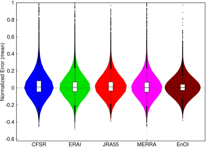
After the application of both data assimilation methods (OI and EnOI), a comparison was first carried out at the stations that were used to update the initial fields. Figure 1.7 in the article compares the performance of OI and EnOI methods for each CPI. It can be seen that reanalysis performance depends on considered CPI and that EnOI datasets outperformed OI applied to each reanalysis independently. NRMSD values (averaged over all CPI) (see equation 1.13) for each year are presented in Figure 1.8 which confirms how the EnOI approach outperformed OI applied to each reanalysis for each year. Violin plots (Hintze & Nelson, 1998) were used to compare the density distribution of NE (see equation 3.4) for each dataset after the application of OI and EnOI; Figure 4.1). Box plots were also added to this figure. It is possible to see that, for each dataset, the median value is close to 0 (values close to 0 and small dispersion around it, represent better agreement with the observations). EnOI globally outperformed the other datasets with the smallest dispersion around 0. It can also be observed, as pointed out in the article (Figure 1.8) that EnOI performance is followed by JRA55, ERAI, MERRA and CFSR respectively. Cross-validation was then applied in order to assess the performance of OI and EnOI at points that were not used to upgrade the initial field (see more details in section 1.7). Figure 1.10 of the article compares MAE (see equation 1.14) for each index, configuration and datasets after applying the data assimilation methods compared with the initial fields. It can be seen that for each CPI and cross-validation network Near or Far
16
(and therefore even for points far away from the calibration network), estimated CPI fields were improved after applying OI or EnOI compared to the reanalysis values.
-0.6 -0.4 -0.2 0 0.2 0.4 0.6 0.8 1
CFSR ERAI JRA55 MERRA EnOI
Normalized Error (mean)
Figure 4.1 – Violin and box plots showing the NE (averaged over all ten indices) after the application of the data assimilation techniques. Boxes represent inter-quartiles range (first, Q1 and third, Q3), line inside the box the median value and outliers correspond to the black dots. Outliers are defined as values 1.5 times the interquartile distance (IQR=Q3-Q1) (whiskers) above or below Q3 or Q1 respectively.
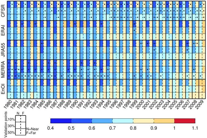
In order to see the general improvements for each year over the study period, Figure 4.2 shows a heatmap of the annual values of V defined by:
V = 1 k k X i=1 M AEA(i) M AEB(i) (4.1)
where M AEA is the Mean Absolute Error of the modified field (reanalysis after applying OI or
EnOI), M AEB the Mean Absolute Error of the initial field (reanalysis for OI or average of all reanalyses for EnOI) and k the number of CPI (k = 10). Each value of the heatmap (V ) therefore corresponds to the mean V value over all CPI for Near or Far configurations with 10, 30, or 50% validation sites for a given year. It can be seen that for each year and each Near or Far network (and
Chapter 4. Results and discussion 17
therefore even for sites far away from the calibration network), estimated CPI fields were improved after applying OI or EnOI compared to the reanalysis values (all V values are smaller than one). Comparing the amplitudes of these improvements between the datasets for each subnetwork (Near or Far with 10, 30 or 50% validation sites) was carried out. It can be observed that CFSR is the reanalysis which displayed the largest improvements (compared with the initial field) over many years followed by MERRA. This figure complements the analysis presented in the article (Figure 1.10) where each CPI was analyzed independently over the study period and similar behaviours were observed (CPI fields were improved and the largest improvements were mostly concentrated between CFSR and MERRA).
CFSR ERAI JRA55 MERRA EnOI 198019811982198319841985198619871988198919901991199219931994199519961997199819992000200120022003200420052006200720082009 N F 10% 30% 50% N=NearF=Far Validation points 0.4 0.5 0.6 0.7 0.8 0.9 1 1.1
Figure 4.2 – Annual values of V (see equation 4.1) after applying OI to each reanalysis (top 12 rows) and after applying EnOI (bottom four rows) averaged over all CPI for the various cross-validation subnetworks (Near and Far configurations with 10, 30 and 50% validation sites). Black dots correspond to the datasets with the largest improvements for a given cross-validation subnetwork.
A comparison between each dataset was carried out. Figure 1.11 in the article summarizes the results of this comparison and shows that the ensemble approach outperforms the different reanalyses updated by OI in most cases. The dataset generated by the EnOI method was finally compared with the gridded dataset of NRCan. Figures 1.12 and 1.13 compare both datasets through three
18
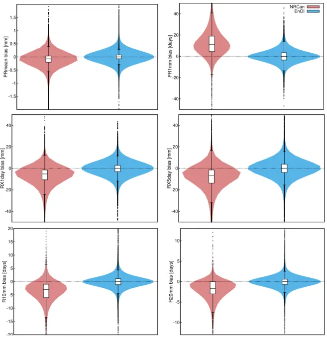
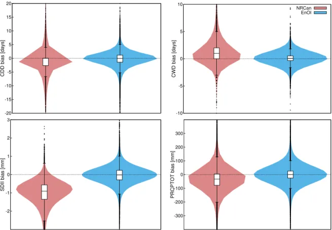
indices (PRmean, PR1mm and RX1day), showing that the CPI estimated from the EnOI dataset outperform NRCan. Figures 4.3 and 4.4 show the violin plots providing the density distribution of the differences or the errors (data minus observation) for each index.
-1.5 -1 -0.5 0 0.5 1 1.5 PRmean bias [mm] -40 -20 0 20 40 PR1mm bias [days] NRCan EnOI -40 -20 0 20 40 RX1day bias [mm] -40 -20 0 20 40 RX5day bias [mm] -20 -15 -10 -5 0 5 10 15 20 R10mm bias [days] -10 -5 0 5 10 R20mm bias [days]
Figure 4.3 – Violin plots showing the bias between EnOI or NRCan and observed values at all the
stations for PRmean, PR1mm, RX1day, RX5day, R10mm and R20mm. Boxes represent inter-quartiles range (first, Q1 and third, Q3), line inside the box the median value and outliers correspond to the black dots. Outliers are defined as values 1.5 times the interquartile distance (IQR=Q3-Q1) (whiskers) above or below Q3 or Q1 respectively.
It can be seen how the EnOI dataset outperforms NRCan for all indices (median values close to 0 and higher violin plot density around 0). NRCan dataset generally underestimates observed
Chapter 4. Results and discussion 19 -20 -15 -10 -5 0 5 10 15 20 CDD bias [days] -10 -5 0 5 10 CWD bias [days] NRCan EnOI -2 -1 0 1 2 3 SDII bias [mm] -300 -200 -100 0 100 200 300 PRCPTOT bias [mm]
Figure 4.4 – Violin plots showing the bias between EnOI or NRCan and observed values at all the stations for CDD, CWD, SDII and PRCPTOT. Boxes represent inter-quartiles range (first, Q1 and third, Q3), line inside the box the median value and outliers correspond to the black dots. Outliers are defined as values 1.5 times the interquartile distance (IQR=Q3-Q1) (whiskers) above or below Q3 or Q1 respectively.
values for extreme indices such as RX1day, RX5day, R10mm, R20mm, SDII and PRCPTOT while it overestimates them for PR1mm and CWD. For CDD, median biases for NRCan are close to 0 but more dispersed than corresponding EnOI values. However, despite PRmean (from NRCan) shows underestimations compared to the observations, these remained small. These results are complementary to those presented in the article (section 1.8.3). Based on these results, it is recommended to use the NRCan dataset with caution for extreme precipitation estimation.
Chapter 5
Summary and Conclusions
Station network density in remote regions of Canada is small. It can be a huge challenge when defining a reliable reference climate datasets by using only this information. Reanalyses represent an interesting option that could be useful for those regions, as they provide consistent spatio-temporal gridded datasets. However, precipitation remains a problematic variable because it is a direct output of the numerical model and observations for this variable have not been explicitly used to create the reanalyses. Data assimilation techniques are interesting alternatives to achieve the goal of combining models outputs and observations in order to define a historical reference dataset.
The OI and EnOI methods were applied to improve the quality of the historical climate precipitation indices for Canada for a reference period of 30 years (1980-2009) where different reanalysis datasets (Climate Forecast System Reanalysis [CFSR], ERA-Interim [ERAI], Japanese 55-year [JRA55] and Modern Era Reanalysis for Research and Applications [MERRA]) were combined with observational data (Daily precipitation records from the Adjusted and Homogenized Canadian Climate Data [AHCCD] developed by Environment Canada and from the stations operated by Ministère du Développement Durable, de l’Environnement et de la Lutte contre les Changements Climatiques [MDDELCC] from Quebec). Precipitation gridded dataset from Natural Resources Canada (NRCan) generated from stations records was also used, mainly for comparison purpose.
A group of ten CPI (defined by the Expert Team on Climate Change Detection and Indices [ETCCDI]) were analyzed, characterizing different features of precipitation or events that occur
22
at least once a year. Annual CPI series were considered in order to maximize the effective use of available observational datasets. Each reanalysis was then combined with the observational dataset using the OI approach while the EnOI method was applied combining the four reanalyses with the observational dataset.
A first analysis was performed aiming at comparing the OI and EnOI datasets at the same observation points and after by a cross-validation strategy. The estimated CPI show improvements compared to the initial fields, increasing also our ability to estimate them with some improvements at ungauged sites. The major improvements were obtained with the ensemble approach compared to the OI for each reanalysis independently. The climate precipitation indices obtained by the ensemble approach were regionally compared with the NRCan dataset, showing that NRCan should be used with caution, especially for extremes. The proposed dataset increases our ability to characterize the current climate in Canada and contributes to the development of climate change impact studies and adaptation strategies.
Part II
Article 1
Defining a reference climate for
Canada through the combination of
observational and reanalysis datasets
Définition d’un climat de référence pour le Canada par la combinaison des ensembles de données d’observation et de réanalyse.
Authors
Alexis Pérez Bello, Alain Mailhot
Institut National de la Recherche Scientifique (INRS), Centre Eau Terre Environnement (ETE), Québec city, Québec, Canada.
Author contribution statement
Prof. Alain Mailhot conceived, proposed and directed the presented work. Mr. Alexis Pérez Bello was responsible of implementation, adaptation and application of the methodology in a computational framework as well as analyzing and processing the different datasets to address the problematic presented. The results were analyzed and discussed by both authors. Mr. Alexis Pérez Bello was also responsible of writing the draft of the manuscript with important critical revisions and feedbacks from Prof. Alain Mailhot.
26
Résumé traduit
La définition d’un climat de référence est un enjeu important pour le développement des futures stratégies d’impact et d’adaptation des changements climatiques. Cela reste encore un défi dans les régions où historiquement la couverture par des stations météorologiques est faible (p.ex. le Nord du Canada). Les réanalyses représentent une option intéressante pour réaliser cet objectif. Cependant, en considérant les biais et les inexactitudes des différentes réanalyses présentement disponibles, une validation et une correction de biais de ces ensembles de données sont encore nécessaires avant qu’ils puissent être utilisés. Dans cette étude, deux méthodes d’assimilation des données ont été considérées pour améliorer les champs climatiques de référence au Canada. Les méthodes d’interpolation optimale (OI pour Optimal Interpolation) et d’interpolation optimale d’ensemble (EnOI pour Ensemble Optimal Interpolation) ont été utilisées pour combiner quatre ensembles de données de réanalyses (CFSR, Era-Interim, JRA55 et MERRA) avec deux ensembles de données d’observation. Un total de 2160 stations météorologiques ayant au minimum 10 années valides d’enregistrements de précipitations et des données sur grille de Ressources Naturelles Canada ont été utilisées. Les valeurs annuelles de dix indices de précipitations climatiques (CPI pour Climate Precipitation Indices) couvrant une période de 30 ans (1980-2009) ont été estimées pour chaque ensemble de données et ont ensuite été combinées (réanalyse + observations) pour améliorer la représentation de chaque indice climatique au Canada. Une stratégie de validation croisée a finalement été appliquée et a montré que l’ensemble de données de référence développé améliore la capacité à estimer les indices climatiques aux endroits où aucune précipitation enregistrée n’est disponible. L’ensemble de données proposé a également été comparé à l’ensemble de données d’observation sur grille de Ressources Naturelles Canada (NRCan). Les résultats ont montré que l’ensemble de données NRCan devrait être utilisé avec prudence, en particulier pour les indices de précipitations extrêmes et dans les régions éloignées.
1.1
Abstract
Defining a reference climate is an important issue for climate change impact and the development of adaptation strategies. This remains a challenge in regions that were historically poorly covered by meteorological stations, such as Northern Canada. Reanalyses represent an interesting option to define a reference climate in such regions. However considering the bias and inaccuracies of the
Article 1. Defining a reference climate by combining observations and reanalysis datasets 27
various reanalyses actually available, some validation and bias-correction of these datasets are still needed before they could be used. In this paper, two data assimilation methods were considered to improve the reference climate fields over Canada. Optimal Interpolation (OI) and Ensemble Optimal interpolation (EnOI) methods were used to combine four reanalysis datasets (CFSR, Era-Interim, JRA55 and MERRA) with observations. A total of 2160 meteorological stations with minimally 10-year precipitation records were used. Annual values of ten Climate Precipitations Indices (CPI) covering a 30-year period (1980-2009) were estimated for each dataset and were then combined (reanalysis + observations) to improve the representation of each climate index across Canada. A cross-validation strategy was finally applied and showed that the developed reference datasets improve our ability to estimate climate indices at sites where no recorded precipitations are available. The proposed dataset (obtained from EnOI) was also compared to the gridded observational dataset from Natural Resources Canada (NRCan). Results showed that NRCan dataset should be used with caution especially for extreme CPI and in remote areas.
1.2
Introduction
In a context of climate change, characterizing historical climate is important to investigate how climate conditions may evolve in the future (Tebaldi et al., 2006; Hatzaki et al., 2010; Westra et al., 2014). Historical climate can be characterized through various indices such has the Climate Precipitations Indices (CPI) proposed by the Expert Team on Climate Change Detection and Indices (ETCCDI) (Peterson et al., 2001; Zhang et al., 2011). These indices have been estimated directly from available observations around the world (e.g., Frich et al. (2002)) and also different gridded datasets of these indices have been produced by interpolating observational datasets (e.g., Alexander et al. (2006); Donat et al. (2013)). If this could be simply done in regions with dense meteorological network operating since many decades, it represents a real challenge in remote regions with short records and low density network as it is the case for many Canadian regions, especially in the northern parts (Mekis & Vincent, 2011).
Reanalyses represent an interesting alternative for such regions as they provide comprehensive and consistent spatio-temporal gridded datasets. Reanalyses consist of a background forecast model and data assimilation routine that combines available observational datasets with model forecast to generate uniform gridded datasets (Bosilovich et al., 2008). They have been widely used in
28
different climate research applications (e.g., Alexeev et al. (2011); Zou et al. (2014); Lindsay et al. (2014)). Extreme indices for precipitation and temperature from reanalyses have also been used as reference for evaluation of climate models (e.g., Sillmann et al. (2013)). Their consistency with global gridded observational datasets have been verified (Donat et al., 2014), showing improvements in representation of the spatial patterns after 1979 when satellite data were included in the assimilation process. Despite their overall good spatio-temporal representation of many variables, some of them (e.g. precipitation) are still not well represented in some regions, mainly because observational datasets for these variables have not been explicitly used in the assimilation process (Saha et al., 2010; Dee et al., 2011; Kobayashi et al., 2015; Rienecker et al., 2011). Evaluating daily climate indices over the northern parts of Canada, Diaconescu et al. (2017) recommend caution when using extreme daily precipitation indices from reanalyses as reference datasets for these regions. Reanalyses therefore need to be bias corrected before they could be used. Their performances depend on the variable considered, the data assimilation routine, the assimilated observational datasets, and the forecast model (Lorenz & Kunstmann, 2012).
One possible option for improving the CPI representation is through the combination of reanalysis datasets with in situ observations through data assimilation methods. These methods combine model fields with observational datasets to create an improved model dataset (Kalnay, 2002; Bertino et al., 2007). They can be incorporated into the modeling process through two different forms: online mode, which increases the quality of the initial conditions sequentially for new model simulations and off-line mode, which is used to create the best estimation, combining the final outputs of the model with observational data (Candiani et al., 2013; Matsikaris et al., 2015).
In this work the off-line mode was applied using the Optimal Interpolation (OI) and Ensemble Optimal Interpolation (EnOI) methods. OI was applied to each reanalysis independently and EnOI to all reanalyses combined. Both methods are quite similar, their main difference being in how the background error covariance is defined (Ren & Hartnett, 2017). These methods were applied because they are relatively straightforward, computational inexpensive and they take into account the uncertainty of the different datasets used. OI method has been used to merge different sources of precipitations in some regions of the world (e.g., Häggmark et al. (2000); Mahfouf et al. (2007); Soci et al. (2016)). Furthermore, significant improvements were obtained with its application at global scale by Nie et al. (2016) merging satellite information with observations and model predictions.
Article 1. Defining a reference climate by combining observations and reanalysis datasets 29
This method has been also used for daily retrospective estimation of streamflow in ungauged rivers by Lachance-Cloutier et al. (2017).
The objective of the paper is to improve the historical CPI datasets for Canada combining observations and reanalyses through the OI and EnOI methods. It is organized as follows. Section 1.3 describes the observational datasets and reanalyses considered in this study. The CPI, data assimilation techniques (OI and EnOI), and the cross-validation procedure are briefly described in Sections 1.4, 1.5, 1.6 and 1.7 respectively. Section 1.8 presents the results followed by a summary and a discussion (Section 1.9).
1.3
Datasets
Five gridded datasets were considered in this study (Table 1.1). The first four ones are widely used reanalyses while the fifth one is the interpolated precipitation dataset from Natural Resources Canada (NRCan) generated from stations records using a thin plate spline smoothing algorithm (ANUSPLIN) (Hutchinson et al., 2009; McKenney et al., 2011). This dataset was used for comparison purpose and to estimate missing values in station records (further details are provided in Section 1.5), also it provides information with good spatial resolution (10 km spatial resolution) which covers Canada (the study domain) and covers a relatively long period (1950 to 2012). Previous studies show underestimation for precipitation values in this dataset (e.g. Hutchinson et al. (2009); Bajamgnigni Gbambie et al. (2017); Diaconescu et al. (2017)). Despite its weaknesses, to our knowledge, there is no other dataset having these characteristics (accessibility, domain size, spatio-temporal resolution and period covered) that can be used for the study area considered in this work. Some other datasets exist but they cover short periods (e.g. CaPA) or cover only Quebec (e.g. MDDELCC dataset; see Bajamgnigni Gbambie et al. (2017)). Since each dataset covers a different period, the common period, 1980-2009, was considered in the following.
Daily precipitation records from the Adjusted and Homogenized Canadian Climate Data (AHCCD) developed by Environment Canada (Mekis & Vincent, 2011) and from the stations operated by Ministère du Développement Durable, de l’Environnement et de la Lutte contre les Changements Climatiques (MDDELCC) from Quebec were also used. Only stations with at least 10 valid years during the 30-year period 1980-2009 were retained. A valid year is defined as a year
30
Table 1.1 – Gridded datasets used in this study (acronyms appearing in parenthesis are used to refer to these datasets).
Gridded datasets Period Spatial resolution Temporal resolution Reference Climate Forecast System Reanalysis (CFSR)
1979-2009 0.312o× 0.312o Hourly Saha et al. (2010)
ERA-Interim
(ERAI) 1979-2012 0.75
o× 0.75o 12 hours Dee et al. (2011)
Japanese 55-year
Reanalysis (JRA55) 1958-2013 0.56
o× 0.56o 3 hours Kobayashi et al. (2015)
Modern-Era Retrospective Analysis for Research and Applications (MERRA)
1979-2012 0.5o× 0.66o Hourly Rienecker et al. (2011)
Precipitation data from Natural Resources Canada
(NRCan)
1950-2012 0.083o× 0.083o Daily McKenney et al. (2011)
with less than 20 % missing daily values (Panthou et al., 2014), for a total of 2160 stations across Canada. Figure 1.1 presents the map of these stations while Figure 1.2 presents the histogram of the number and percentage of stations with given numbers of valid years during the 1980-2009 period. Figure 1.1 clearly shows that stations are unevenly distributed and mainly concentrated in the southern parts of the country. Figure 1.2 confirms that available records contain many missing data (only 10.8 % of the stations have records covering the complete 1980-2009 period).
It is important to note that not all the stations considered in this study were used to create the NRCan dataset (for instance, some stations operated by the MDDELCC in Quebec were not used). Also it is well known that interpolated precipitation, especially extreme values, at daily time scale can be highly uncertain in regions with sparse network coverage (Gervais et al., 2014).
Article 1. Defining a reference climate by combining observations and reanalysis datasets 31
126W
108W
90W
72W
54W
45N
54N
63N
72N
81N
Figure 1.1 – Map of the stations considered in this study.
10 11 12 13 14 15 16 17 18 19 20 21 22 23 24 25 26 27 28 29 30 0 25 50 75 100 125 150 175 200 225 250
Number of valid years
Number of stations 4.6 5.5 5.2 7.9 7.3 6.0 5.4 3.2 2.6 3.1 2.8 2.7 3.2 3.23.0 3.7 3.5 4.5 5.86.0 10.8
Figure 1.2 – Number and percent (above each bar) of stations with given numbers of valid years.
1.4
Climate Precipitation Indices and Super-Observations
Different Climate Precipitation Indices (CPI) defined by the Expert Team on Climate Change Detection and Indices (ETCCDI) as well as mean annual precipitation (PRmean) have been
32
considered in this study (Table 1.2). Annual CPI values were first estimated as well as climatological mean over the 1980-2009 period. CPI were estimated at each native grid point of each dataset (reanalysis or NRCan dataset). A second-order conservative remapping (Jones, 1999) was then applied to each CPI gridded dataset created from ERAI, JRA55 and MERRA using the CFSR grid as reference grid. OI and EnOI methods were applied once CPI gridded datasets from each reanalysis were put on a common grid.
Table 1.2 – Climate Precipitation Indices, adapted from Zhang et al. (2011)
Index Description Units
PRmean Annual mean of daily precipitation. mm
PR1mm Number of wet days (daily precipitation ≥ 1 mm/day). days RX1day Annual maximum 1-day precipitation amount. mm RX5day Annual maximum 5-day precipitation amount. mm
SDII Simple daily intensity index (The ratio of annual total
precipitation to the number of wet days ≥ 1 mm). mm R10mm Annual number of days when precipitation ≥ 10 mm. days R20mm Annual number of days when precipitation ≥ 20 mm. days CDD Annual maximum number of consecutive days when
precipitation is below 1 mm. days
CWD Annual maximum number of consecutive days when
precipitation ≥ 1 mm. days
PRCPTOT Annual total precipitation from days ≥ 1 mm. mm
As shown in Figure 1.1, station density in southern Canada can be high. Observations from neighboring stations can therefore be highly correlated at the daily time scale. Furthermore reanalysis do not properly represent small scale processes (Vihma et al., 2014). Super-observations (Daley, 1991; Oke et al., 2006), also called upscaled observations (Cherubini et al., 2002), were therefore created using the reanalysis grid with the highest resolution as reference grid (i.e. CFSR).
Article 1. Defining a reference climate by combining observations and reanalysis datasets 33
Super-observations values were estimated by combining station values within the same grid cell using the following expression:
x = Pn i=1ViXi Pn i=1Vi (1.1) where n is the number of stations inside a given grid cell, Vi is the number of valid days per station for each year, while Xi represent annual CPI value for year i. Longitude and latitude of the
super-observations were also estimated using a similar expression.
Figure 1.3 shows the number of stations and corresponding super-observation with valid records for each year of the 1980-2009 period. It shows that, after a peak in the 1988-1992, the number of stations quickly decreased to reach a minimum value in 2009. The spatial distribution of the super-observations changes from year to year depending of the number and location of stations available each year. These super-observations networks were finally used to apply OI and EnOI for each year independently.
0 250 500 750 1000 1250 1500 1750 2000 2250 1980 1984 1988 1992 1996 2000 2004 2008
2160 => Total number of Stations
Number of Stations
Years
Stations Super-obs.
34
1.5
Optimal Interpolation (OI)
This section provides a brief description of the Optimal Interpolation (OI) method and how it was applied in this paper. A more general and comprehensive description can be found in Daley (1991); Kalnay (2002); Sen (2009).
Optimal interpolation, also known as statistical interpolation, is a widely used method (e.g., Mahfouf et al. (2007); Lespinas et al. (2015)) to create an analysis field by combining a background state, or model forecast, with the observation network (Daley, 1991). The analysis value ψ(j)A at grid point j is estimated by the background field ψB(j)plus the linear combination of the differences between the observations ψO(i) (i = 1...n) where n is the number of observations close to this grid point and the background values at the observation site ψ(i)B. The so-called analysis equation is defined as:
ψ(j)A = ψB(j)+
n X
i=1
W(j,i)(ψ(i)O − ψB(i)) (1.2)
Assuming that the background error only depends on distance (so-called homogeneous conditions), is independent of the direction (isotropic), and that the observation errors are uncorrelated, then, W , the interpolation weights matrix, can be estimated by the following equation Daley (1991):
[BEC+ µI]W = bEC (1.3)
in which BEC is the background error correlation matrix between the station values, bEC is the
background error correlation vector between the observations and the grid point to analyze from the background field, I is the identity matrix and µ = OEV/BEV where OEV and BEV are the
observation and background error variance respectively. Parameter µ can be adjusted such that the weights granted to observations can be increased or reduced (Kalnay, 2002). OEV and BEV for
each index and reanalysis respectively were estimated according to the methodology described in Section 4.3 of Daley (1991).
The available CPI annual series over the studied 30-year period were used to estimate the spatial dependence of the correlation function BEC(x) in equation (1.3). The values at each observation
point from the background field were obtained for each year by mean of bilinear interpolation and the missing values in the observational dataset were filled out with the CPI calculated from NRCan
Article 1. Defining a reference climate by combining observations and reanalysis datasets 35
dataset. Then, correlations Rij of the differences between the observations and background field at site i and j were calculated using the following equation (Sen, 2009; Daley, 1991):
Rij =
(Oi− Bi)(Oj− Bj) q
(Oi− Bi)2(Oj − Bj)2
(1.4)
where the overlined variable corresponds to average of annual values over the reference period. The mean correlations over each 30-km distance intervals were then computed. Many different spatial correlation functions R(x) were used and the following expression was finally selected and adjusted to the estimated values (Sen, 2009):
R(x) = a + be(−x/c) (1.5)
where x is the distance between stations and a, b and c are fitting parameters. Figure 1.4 shows an example of the mean correlation estimated for each distance interval with the corresponding fit of equation 1.5 for the RX1day index estimated from CFSR.
0 100 200 300 400 500 600 0 0.1 0.2 0.3 0.4 0.5 0.6 0.7 Distance [km] Correlation
Figure 1.4 – Estimated correlation function (continuous curve) with corresponding discrete values for the RX1day from CFSR.
Due to the averaging process over successive intervals, Figure 1.4 shows that zero distance correlation has to be extrapolated. Using equation 1.5 and setting x = 0, the isotropic background error correlation BEC used in equation 1.3 is given by (Sen, 2009):
BEC(x) =
R(x)
R(0) or BEC(x) =
a + be(−x/c)
36
The relative expected analysis error ε for each grid point can be estimated by the following equation (Kalnay, 2002; Sen, 2009; Daley, 1991):
ε = 1 −
n X
i=1
W(i)b(i)EC (1.7)
where values of ε close to 0 means a biggest influence or weight of neighbouring observations in the estimation of the CPI value at this specific grid point while values of ε close to 1 means a biggest contribution of the background field. W and bEC were explained above when equation 1.3 was presented.
1.6
Ensemble Optimal Interpolation (EnOI)
This section provides a brief description of Ensemble Optimal Interpolation (EnOI) method and how it was applied in this paper. A more general and comprehensive description can be found in Evensen (2003).
The EnOI is an approximation of the Ensemble Kalman filter (EnKF) in which an ensemble of model states in long time integration (stationary) is used to compute the analysis in the space spanned and only one model state is used as a background field (Oke et al., 2006). Defining a matrix E with the ensemble members:
E = [M1, M2, ..., Mn] (1.8)
where n is the number of ensemble members which are stored (vector form) in each column of E. For each CPI, the ensemble members are the 30 years of each reanalysis combined (n = 120 members). The anomaly or ensemble perturbation matrix En can be defined by:
En= E − Em (1.9)
where Em is the ensemble mean matrix in which each column has the same ensemble mean vector
calculated from all the ensemble members stored in E. Then, the ensemble covariance matrix ECM can be estimated by:
ECM =
αEnEnT