Analysis and improvement of GNSS navigation message demodulation performance in urban environments

(1)

DOCTORAT DE L'UNIVERSITÉ DE TOULOUSE

Délivré par :

Institut National Polytechnique de Toulouse (INP Toulouse)

Discipline ou spécialité :

Signal, Image, Acoustique et Optimisation

Présentée et soutenue par :

Mme MARION ROUDIER

le vendredi 16 janvier 2015

Titre :

Unité de recherche :

Ecole doctorale :

DEFINITION DE SIGNAUX ET DE TECHNIQUES DE TRAITEMENT

INNOVANTS POUR LES FUTURS SYSTEMES GNSS

Mathématiques, Informatique, Télécommunications de Toulouse (MITT)

Laboratoire de Traitement du Signal et des Télécommunications - LTST, à l'ENAC

Directeur(s) de Thèse :

M. OLIVIER JULIEN

MME MARIE LAURE BOUCHERET

Rapporteurs :

M. EMMANUEL BOUTILLON, UNIVERSITE DE BRETAGNE SUD M. MARCO LUISE, UNIVERSITA DI PISA

Membre(s) du jury :

1 M. EMMANUEL BOUTILLON, UNIVERSITE DE BRETAGNE SUD, Président

2 M. AXEL GARCIA PENA, ECOLE NATIONALE DE L'AVIATION CIVILE, Membre

2 M. CHARLY POULLIAT, INP TOULOUSE, Membre

2 M. CHRISTOPHER HEGARTY, THE MITRE CORPORATION BEDFORD, Membre

2 M. MATTEO PAONNI, IPSC, Membre

2 Mme MARIE LAURE BOUCHERET, INP TOULOUSE, Membre

(2)

1

Abstract

Global Navigation Satellite Systems (GNSS) are increasingly present in our everyday life. New users are emerging with further operational needs implying a constant evolution of the current GNSS systems. A significant part of the new applications are found in environments with difficult reception conditions such as urban areas, where there are many obstacles such as buildings or trees. Therefore, in these obstructed environments, the signal emitted by the satellite is severely degraded. The signal received by the user has suffered from attenuations, as well as refractions and diffractions, making difficult the data demodulation and the user position calculation.

GNSS signals being initially designed in an open environment context, their demodulation performance is thus generally studied in the associated AWGN propagation channel model. But nowadays, GNSS signals are also used in degraded environments. It is thus essential to provide and study their demodulation performance in urban propagation channel models.

Nevertheless, GNSS modernization with new signals design such as GPS L1C or Galileo E1 OS, takes into account these new obstructed environments constraints. Since they have been designed especially for urban propagation channels [1], they are expected to have better demodulation performance compared with current GNSS signals. It is thus particularly interesting to firstly provide their demodulation performance in urban environments (not available in the literature) and secondly to compare it with the new GNSS signal designed in this PhD research context. In this way, their performance could be used as a benchmark for the future signals design.

However these modernized signals are not yet available for this moment (for example, GPS L1C is expected to be operational over the entire constellation in 2026). It is thus essential to provide and study their demodulation performance in urban environments through simulations.

It is in this context that this PhD thesis is related, the final goal being to improve GNSS signals demodulation performance in urban areas, proposing a new signal.

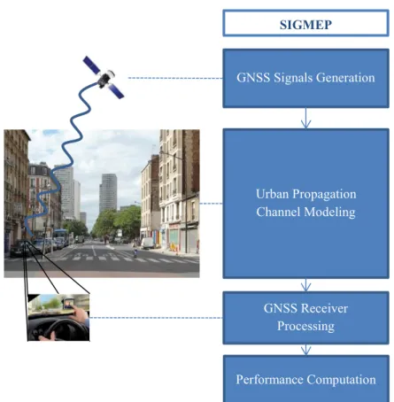
In order to be able to provide and study GNSS signals demodulation performance in urban environments, a simulation tool has been developed: SiGMeP for ‘Simulator for GNSS Message Performance’. It allows simulating the entire emission/reception GNSS signal chain in urban environment getting away from dependence of real signals availability, controlling the simulation parameters and testing new configurations.

Existing and modernized signals demodulation performance has thus been computed with SiGMeP in urban environments. Since the classical way to compute and represent GNSS signals demodulation performance assumes an AWGN propagation channel model, and since the urban environments are really different from the AWGN channel, this classical method is not satisfactory in our urban context.

(3)

2

Thus, in order to represent GNSS signals demodulation performance faithfully to reality, a new methodology more adapted to the user environment is proposed. It is based on the fundamental characteristics of a GNSS system, as well as on the urban environment impact on the received signal analysis. GNSS signals demodulation performance is thus provided in urban environments thanks to this new methodology, and compared with the classic methodology used in the AWGN case.

Then, to improve GNSS signals demodulation performance in urban environments, many strategies are possible. However, the research axis of this thesis focuses on the ‘Channel Coding’ aspect. It is thus this field which will be privileged to improve GNSS signals demodulation performance in urban environments.

Each message, in addition to containing the useful information, carries redundant information, which is in fact the channel coding result, applying to the useful information. The message thus needs to be decoded at the reception. In order to decode the transmitted useful information, the receiver computes a detection function at the decoder input. But the detection function used in classic receivers corresponds to an AWGN propagation channel. This dissertation thus proposes an advanced detection function which is adapting to the propagation channel where the user is moving. This advanced detection function computation considerably improves demodulation performance, just in modifying the receiver part of the system.

Finally, in order to design a new signal with better demodulation performance in urban environments than one of existing and future signals, a new LDPC channel code profile has been proposed, optimized for a CSK modulation in an AWGN channel for iterative decoding. Indeed, the CSK modulation is a promising modulation in the spread spectrum signals world, which permits to free from limitations in terms of data rate implied by current GNSS signals modulations. Moreover, LDPC codes belong to the modern codes family, the first being able to approach the channel capacity. They thus represent promising achievable performance.

(4)

3

Résumé

Les systèmes de navigation par satellites sont de plus en plus présents dans notre vie quotidienne. De nouveaux utilisateurs émergent, avec des besoins différents, ce qui implique une évolution constante des systèmes de navigation par satellites actuels. La majorité de ces nouveaux besoins concernent des applications en environnement urbain. Dans ce type d’environnement très obstrué, le signal reçu par l’utilisateur a subit des atténuations ainsi que des réfractions/diffractions, ce qui rend difficile la démodulation des données et le calcul de position de l’utilisateur.

Les signaux de navigation par satellites étant initialement conçus dans un contexte d’environnement dégagé, leurs performances de démodulation sont donc généralement étudiées dans le modèle de canal de propagation AWGN associé. Or aujourd’hui ils sont utilisés aussi en environnements dégradés. Il est donc indispensable de fournir et d’étudier leurs performances de démodulation dans des modèles de canal de propagation urbain.

C’est dans ce contexte que s’inscrit cette thèse, le but final étant d’améliorer les performances de démodulation des signaux GNSS en milieux urbains, en proposant un nouveau signal.

Afin de pouvoir fournir et analyser les performances de démodulation des signaux de navigation par satellite en milieux urbains, un outil de simulation a été développé dans le cadre de cette thèse : SiGMeP pour « Simulator for GNSS Message Performance ». Il permet de simuler la chaine entière d’émission/réception d’un signal de navigation par satellites et de calculer ses performances de démodulation en milieu urbain.

Les performances de démodulation des signaux existants et modernisés ont donc été calculées avec SiGMeP en environnement urbain. Afin de représenter au mieux ces performances pour qu’elles soient le plus réalistes possibles, une nouvelle méthode est proposée dans ce manuscrit. Elle se base sur les caractéristiques fondamentales d’un système de navigation par satellites, ainsi que sur l’analyse de l’impact d’un environnement urbain sur le signal reçu. Les performances de démodulation des signaux en environnement urbains sont donc fournies à travers cette nouvelle méthodologie, et comparer à la méthodologie classique utilisée dans le cas AWGN.

Ensuite, pour améliorer ces performances de démodulation des signaux de navigation par satellites, plusieurs stratégies sont envisageables. Cependant, l’axe de recherche de cette thèse est centré sur l’aspect « codage canal ». C’est donc ce domaine d’étude qui sera privilégié.

Chaque message, en plus de contenir l’information utile, transporte de l’information redondante, qui est en fait le résultat du codage canal appliqué sur l’information utile. Ainsi à la réception, le message de navigation doit être décodé, afin que le récepteur retrouve l’information utile transmise. Pour décoder l’information utile transmise, le récepteur calcule une fonction de détection à l’entrée du

(5)

4

décodeur. Or la fonction de détection utilisée dans les récepteurs classiques correspond à un modèle de canal AWGN. Ce manuscrit propose donc une fonction de détection avancée, qui s’adapte au canal de propagation dans lequel l’utilisateur évolue, ce qui améliore considérablement les performances de démodulation, en ne modifiant que la partie récepteur du système.

Enfin, dans le but de concevoir un nouveau signal avec de meilleures performances de démodulation en environnement urbain que celles des signaux existants ou futurs, un nouveau codage canal de type LDPC a été optimisé pour une modulation CSK. En effet, la modulation CSK est une modulation prometteuse dans le monde des signaux de type spectre étalé, qui permet de se débarrasser des limitations en termes de débit de données qu’impliquent les modulations actuelles des signaux de navigation par satellites. Ainsi, la conception d’un code LDPC optimisé pour un signal de navigation par satellite modulé en CSK a été examinée.

(6)

5

Acknowledgements

J’aimerais tout d’abord remercier les personnes qui m’ont permis de faire cette thèse : Christophe Macabiau qui me l’a proposée, et Damien Kubrak qui m’a convaincue de le faire (et tous les autres que j’ai interrogés sans retenue, et qui, avec leurs réponses très sincères m’ont également bien aidée dans mon choix).

Ensuite bien sûr je remercie mes encadrants : Axel Garcia-Pena, qui au quotidien m’a aidée, expliquée (parfois plusieurs fois la même chose, et sans jamais s’énerver…), soutenue et comprise, Olivier Julien, qui même très occupé a toujours su trouver du temps pour moi, pour m’orienter, me corriger, me conseiller (et pas uniquement sur le sujet de la thèse), et Charly Poulliat qui m’a accompagnée dans ce monde nouveau des « Comm Num », qui m’a énormément appris, même si l’on ne s’est pas vus très souvent finalement. Merci de ne pas m’avoir abandonnée, surtout ce weekend du 11 novembre dont je me souviendrai très longtemps ! Merci également à Marie-Laure Boucheret.

Je tiens également à remercier les financeurs de cette thèse : Thales Alenia Space et le CNES. Merci à Lionel Ries et Thomas Grelier d’avoir suivi l’avancement de mon travail. Et c’est avec grand plaisir que l’aventure continue avec le CNES !

I also gratefully acknowledge my three reviewers: Emmanuel Boutillon, Marco Luise and Christopher Hegarty for reviewing my thesis, and in addition Matteo Paonni, for attending my defense.

Je remercie aussi très chaleureusement le laboratoire SIGNAV de l’ENAC. C’est en partie grâce aux gens formidables de ce laboratoire que j’en suis là aujourd’hui. Et merci à tous mes collègues grâce à qui l’ambiance a été si bonne : Jérémy (tous les deux dans la même galère …), Anaïs (ma compère de footing, bon d’accord il n’y en a pas eu beaucoup… et surtout de potins !), Antoine (ses chemises, son humour, et son attachant décalage), Rémi (plus qu’un collègue, merci pour les vraies discussions…), Ludovic (mon co-bureau et mon co-légumes !), Kevin (qui me faisait très peur quand il travaillait comme un fou sur la rédaction de sa thèse, je m’étais dit : moi jamais ça ! Mais oui bien sûr…), Jimmy (mon frère breton, vive le beurre salé !), Enik, Alexandre, Christophe, Paul, les petits nouveaux Alizé, Giuseppe, Quentin, J-B… C’est avec un gros pincement au cœur que je vous quitte.

Et pour finir merci à ma famille. Merci à mes parents de m’avoir toujours soutenue, c’est grâce à vous si j’en suis là, tant logistiquement que moralement. Merci pour votre dévouement, pour votre confiance, et pour m’avoir toujours poussée. Merci aussi à ma petite sœur, sans qui je ne serai pas

(7)

6

celle que je suis. Et bien évidemment merci à Cyril. Je ne nous ai pas rendu la vie facile avec mes études, et même si physiquement on a souvent été séparés, depuis le début tu es là, et ça a énormément compté. Merci d’être toi, tu m’as rendu la vie tellement plus facile… Merci.

(8)

7

List of Figures

Figure 1: GPS L1 C/A signal modulation block diagram ... 27

Figure 2: GPS L1 C/A navigation message general structure ... 28

Figure 3: GPS L1 C/A navigation message word structure ... 28

Figure 4: GPS L1 C/A channel coding description ... 29

Figure 5: GPS L1 C/A encoding process [9] ... 29

Figure 6: GPS L1 C/A decoding process proposed by [9] ... 30

Figure 7: Existing and planned SBAS systems [11] ... 30

Figure 8: SBAS message structure ... 31

Figure 9: SBAS channel encoding description ... 32

Figure 10: SBAS convolutional encoder [9] ... 33

Figure 11 : Multiplexing process for CM and CL PRN codes ... 34

Figure 12: GPS L2C signal modulation block diagram ... 34

Figure 13: GPS L2C navigation message general structure ... 35

Figure 14: GPS L2C channel encoding description ... 36

Figure 15 : Galileo E1 OS signal modulation block diagram ... 38

Figure 16: Galileo E1 OS nominal subframes structure [17] ... 40

Figure 17: I/NAV nominal page structure [17] ... 41

Figure 18: Galileo interleaver description [17] ... 42

Figure 19: Performance of FEC techniques used in GPS and Galileo data messages [10] ... 43

Figure 20: CED error rate as function of the total signal C/N0 in the AWGN channel [10] ... 44

Figure 21: CED error rate as function of the total signal C/N0 in the urban channel [10] ... 44

Figure 22: GPS L1C signal modulation block diagram ... 46

Figure 23: GPS L1C navigation message structure... 47

Figure 24: BCH encoder for the subframe 1 of the GPS L1C message [19]... 48

Figure 25: GPS L1C subframe 2 channel encoding description ... 48

Figure 26: GPS L1C subframe 3 channel encoding description ... 48

Figure 27: Parity-check matrix of the GPS L1C message subframe 2 ... 49

(13)

12

Figure 29: Resulting LDPC encoded subframes ... 50

Figure 30: EER comparison between GPS L1C and GALILEO E1 OS signals for a mobile channel transmission with a receiver travelling at 30 km/h [4] ... 51

Figure 31 : Classical encoder representation ... 52

Figure 32: Tanner graph associated to the H matrix example ... 55

Figure 33: BP algorithm illustration ... 57

Figure 34: Generation of samples following a Loo distribution ... 64

Figure 35: First-order Markov chain state transitions process ... 65

Figure 36: Semi-Markov chain state transitions process ... 66

Figure 37: Generation of Loo samples for the Prieto channel model ... 67

Figure 38: Amplitude and phase of the Prieto channel model simulated samples ... 68

Figure 39: Scene example generated by the DLR propagation channel model [36] ... 69

Figure 40: Synthetic environment [35] ... 70

Figure 41: a) DLR channel model CIR example, with 0° of azimuth angle - b) Amplitude and phase of the DLR channel model simulated samples, with 0° of azimuth angle ... 72

Figure 42: a) DLR channel model CIR example, with 45° of azimuth angle - b) Amplitude and phase of the DLR channel model simulated samples, with 45° of azimuth angle ... 72

Figure 43: a) DLR channel model CIR example, with 90° of azimuth angle - b) Amplitude and phase of the DLR channel model simulated samples, with 90° of azimuth angle ... 73

Figure 44: Real GNSS receiver block diagram ... 78

Figure 45: Main processing block for acquisition and tracking processes ... 79

Figure 46: Spreading code autocorrelation functions for different modulations ... 81

Figure 47: Simulation of a GNSS signal transmission/reception chain by SiGMeP ... 86

Figure 48: Simulation tool SiGMeP structure presentation ... 86

Figure 49: PLL operation between the data and pilot components in SiGMeP ... 89

Figure 50: SiGMeP correlator output modeling ... 92

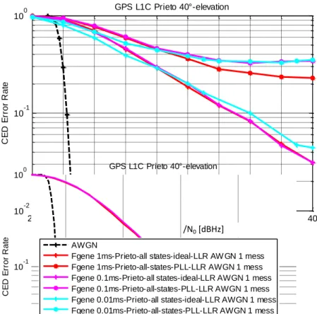
Figure 51: GPS L1C demodulation performance in the Prieto model for different propagation channel generation frequencies ... 97

Figure 52: GNSS signals demodulation performance in the AWGN channel model with the classical methodology ... 101

Figure 53: Comparison between the useful received signal power C and the received direct signal power without channel attenuation Cpre-urban ... 102

Figure 54: The received signal amplitude with the Prieto channel model ... 104

Figure 55: The received signal phase with the Prieto channel model ... 104

Figure 56: The correlator outputs Ip with the Prieto channel model ... 105

Figure 57: ‘Favorable state messages’ histogram and associated statistical values, for GPS L1C in the Prieto channel model with 40° of elevation considering the Prieto channel GOOD states as favorable reception conditions ... 107

(14)

List of Figures

13 Figure 59: GPS L1C GOOD state CED demodulation performance and total CED demodulation performance

with the Prieto model and emitting satellite elevation angle equal to 40°... 115

Figure 60: ‘Favorable state messages’ histogram, for GPS L1C in the Prieto channel model with 80° of elevation considering the Prieto channel GOOD states as favorable reception conditions ... 117

Figure 61: GPS L1C GOOD state CED demodulation performance and total CED demodulation performance with the Prieto model and emitting satellite elevation angle equal to 40° and 80°, considering a PLL tracking 118 Figure 62: GPS L1C and Galileo E1 OS GOOD state CED demodulation performance and total CED demodulation performance with the Prieto model and emitting satellite elevation angle equal to 40°, considering a PLL tracking ... 119

Figure 63: ‘Favorable state messages’ histogram, for Galileo E1 OS in the Prieto channel model with 40° of elevation considering the Prieto channel GOOD states as favorable reception conditions ... 120

Figure 64: ‘Favorable state messages’ determination through the received C/N0 estimation ... 122

Figure 65: Distribution of the degradation between the Cpre-urban/N0 value and the minimum estimated received C/N0 over 1 message, for Cpre-urban/N0 = 25 dB-Hz and PLL tracking with the DLR model ... 123

Figure 66: Cumulative distribution function of the degradation between the Cpre-urban/N0 value and the minimum estimated received C/N0 over 1 message, for Cpre-urban/N0 = 25 dB-Hz and PLL tracking with the DLR model . 123 Figure 67: Favorable states message over 1 hour distribution with 3.4% of average availability, for Cpre-urban/N0 = 25 dB-Hz and PLL tracking, with the DLR model ... 124

Figure 68: GPS L1C favorable states CED demodulation performance and total demodulation performance with the DLR model ... 125

Figure 69: ‘Favorable state messages’ determination through the received C/N0 estimation ... 127

Figure 70: Cumulative distribution function of the degradation between the Cpre-urban/N0 value and the minimum estimated received C/N0 over 1 message, for Cpre-urban/N0 = 37 dB-Hz and PLL tracking, with the Prieto model ... 128

Figure 71: Favorable states subframe 3 demodulation performance and total demodulation performance with the Prieto model ... 129

Figure 72: Favorable state messages over 1 hour distribution, for Cpre-urban/N0 = 37 dB-Hz and PLL tracking with the Prieto model ... 130

Figure 73: Favorable states subframe 3 demodulation performance and total demodulation performance with the DLR model ... 131

Figure 74: Favorable state messages over 1 hour distribution, for Cpre-urban/N0 = 29 dB-Hz and PLL tracking with the DLR model ... 132

Figure 75: GNSS receiver block diagram ... 136

Figure 76: GNSS emission/reception chain block diagram ... 137

Figure 77: GPS L1C demodulation performance obtained with 𝐿𝐿𝑅𝐴𝑊𝐺𝑁 in the Prieto channel model ... 145

Figure 78: Channel bad state duration distribution ... 146

Figure 79: Channel good state duration transition ... 146

Figure 80: GPS L1C demodulation performance obtained with 𝐿𝐿𝑅𝑝𝑒𝑟𝑓𝑒𝑐𝑡 𝐶𝑆𝐼 in the Prieto channel model ... 147

Figure 81: GPS L1C demodulation performance obtained with 𝐿𝐿𝑅𝑛𝑜 𝐶𝑆𝐼 in the Prieto channel model ... 148

Figure 82 : GPS L1C demodulation performance obtained with advanced detection functions in the Prieto channel model ... 149

(15)

14

Figure 84: CSK waveforms example ... 153

Figure 85: CSK FFT-based demodulator representation... 155

Figure 87: CSK demodulator soft inputs and outputs ... 159

Figure 89: CSK demodulator and LDPC decoder combination, linked by LLR exchanged messages, for the classical decoding method ... 161

Figure 90: CSK demodulator and LDPC decoder combination, linked by LLR exchanged messages, for the iterative decoding method ... 162

Figure 92: 10 bits CSK symbol EXIT charts for different Es/N0 ... 167

Figure 93: CSK EXIT charts for different numbers of bits per CSK symbols ... 168

Figure 94: Comparison between the maximum achievable code rate 𝑅0with iterative and non-iterative decoding, for a CSK symbol composed of 10 bits ... 170

Figure 95: Exchanged messages evolution for one iteration ... 171

Figure 96 : CN updating (reference to Chapter 2)... 173

Figure 97: Achievable rate for different maximum variable node degrees for the 2 bits per CSK symbol case 177 Figure 98: Achievable rate for different maximum variable node degrees for the 6 bits per CSK symbol case 178 Figure 99: Finite length results: BER according to Eb/N0 for 2 bits per CSK symbol and 6 bits per CSK symbol ... 179

Figure 100: GNSS signals demodulation performance in the AWGN channel model with the classical methodology ... 193

Figure 102: Code rate definition ... 199

Figure 103 : Source and corresponding output through a propagation channel ... 200

Figure 104: Capacity limits on the BER performance for codes with different rates operating over a binary input AWGN channel [62] ... 201

Figure 105: Shannon Sphere-Packing Lower Bounds on the WER Performance for Codes with Varying Information Block Length k and Rates 1/6, 1/4, 1/3, 1/2, Operating over an Unconstrained-Input AWGN Channel [62] ... 202

Figure 106: Concatenated code architecture ... 203

Figure 107: Conceptual Block Interleaver [19] ... 205

Figure 108: Interleaving depth ... 206

Figure 109: Bit Error Rate Simulated Performance of the CCSDS Concatenated Scheme with Outer E=16 Reed-Solomon Code (255,223) and Inner Rate-1/2 Convolutional Code as a Function of Interleaving Depth [62] ... 206

(16)

15

List of Tables

Table 1: The GPS L2C navigation message types [9] ... 36

Table 2: Galileo navigation message types ... 39

Table 3: I/NAV word types according to the contained data ... 41

Table 4: LDPC channel coding background ... 52

Table 5: BP algorithm description ... 58

Table 6: Databases for the Perez-Fontan model ... 60

Table 7: Direct signal component correlation time examples ... 62

Table 8: Multipath component correlation time examples ... 62

Table 9: Multipath component Doppler spread examples ... 63

Table 10: Loo parameters generation ... 67

Table 11: Simulated conditions for the Prieto channel model ... 67

Table 12: Characteristics for the DLR measurement campaign ... 69

Table 13: Simulated conditions for the Prieto channel model ... 72

Table 14: Main different characteristics between the Perez-Fontan/Prieto and DLR propagation channel models ... 73

Table 15: Spreading code sequence duration for several GNSS signals ... 80

Table 16: SiGMeP PLL parameters ... 90

Table 17: Receiver oscillators parameters for the PLL phase noise modeling ... 93

Table 18: Simulated conditions for the propagation channel model ... 94

Table 19: BER and CEDER values as a function of 𝑇𝐼𝑝𝑎𝑟𝑡 for the Prieto propagation channel model ... 94

Table 20: BER degradation for the Prieto propagation channel model ... 95

Table 21: BER and CEDER values as a function of 𝑇𝐼𝑝𝑎𝑟𝑡 for the DLR propagation channel model ... 95

Table 22: BER degradation for the Prieto propagation channel model ... 96

Table 23: BER values as a function of receiver clock for the AWGN propagation channel model ... 98

Table 24: Simulation conditions for the Perez-Fontan/Prieto propagation channel model ... 103

Table 25: New methodology ... 105

Table 26: Strategy n°1 ... 110

Table 27: Strategy n°2 ... 110

(17)

16

Table 29: Operational requirement example ‘low level’ interpretation through the strategy n°1 ... 113

Table 31: Simulation conditions for the DLR propagation channel model ... 122

Table 32: Strategy n°2 operational requirement example ... 126

Table 33: Operational requirement example interpretation through the strategy n°2 ... 126

Table 35: GA for the Perez-Fontan/Prieto model, for Cpre-urban/N0 = 37 dB-Hz... 130

Table 36: Simulation conditions for the DLR propagation channel model ... 131

Table 37: GA for the DLR model, for Cpre-urban/N0 = 29 dB-Hz ... 132

Table 38: Simulation conditions ... 144

Table 39: Time durations used to compute the estimated received C/N0 ... 145

(18)

17

Abbreviations

ADC Analog to Digital Converter APP A Posteriori Probability

AWGN Additive White Gaussian Noise BER Bit Error Rate

BICM Bit Interleaved Coded Modulation BOC Binary Offset Carrier

BP Belief-Propagation bps bits per second

BPSK Binary Phase-shift keying CBOC Composite Binary Offset Carrier CDDS Commercial Data Distribution Service CED Clock and Ephemeris Data

CEDER Clock and Ephemeris Data Error Rate CIR Channel Impulse Response

CN Check Node

CNAV Civil NAVigation CRC Cyclic Redundancy Check CSI Channel State Information CSK Code Shift Keying

DLR German Aerospace Center

DS-SS Direct Sequence Spread Spectrum

EGNOS European Geostationary Navigation Overlay Service ER Error Rate

EXIT EXtrinsic-Information-Transfer FLL Frequency-locked loop

GIOVE Galileo In-Orbit Validation Element GNSS Global Navigation Satellites System GPS L1 C/A: GPS L1 Coarse/Acquisition IF Intermediate Frequency

(19)

18

IRA Irregular Repeat Accumulate LDPC Low-Density Parity-Check LLR Log Likelihood Ratio LMS Land-Mobile Satellite LNA Low Noise Amplifier LOS Line-Of-Sight

LSB Least Significant Bits LSR Linear Shift Register MAP Maximum A Posteriori

MBOC Multiplexed Binary Offset Carrier ML Maximum Likelihood

MSB Most Significant Bits OS Open Service

pdf Probability Density Function PLL Phase-Locked Loop

PRN Pseudo Random Noise REP Repetition

RF Radio Frequency

RIMS Ranging Integrity Monitoring Stations SBAS Satellite-Based Augmentation System SiGMeP Simulator for GNSS Message Performance SISO Soft Input Soft Output

SNR Signal to Noise Ratio SoL Safety of Life

SPA Sum-Product Algorithm SPC Single Parity Check constraint sps symbols per second

TI Integration Time TOI Tile Of Interval TOW Time Of Week TTFF Time To First Fix

UTC Coordinated Universal Time VCO Voltage-Controlled Oscillator VN Variable Node

(20)

19

PhD Introduction

Chapitre 1:

Background and Motivation

1.1

Global Navigation Satellite Systems (GNSS) are increasingly present in our everyday life. The interest of new users with further operational needs implies a constant evolution of the current GNSS systems. A significant part of the new applications are found in environments with difficult reception conditions such as urban or indoor areas. In these obstructed environments, the received signal is severely impacted by obstacles which generate fast variations of the received signal’s phase and amplitude that are detrimental to both the ranging and demodulation capability of the receiver. One option to deal with these constraints is to consider enhancements to the current GNSS systems, where the design of an innovative signal more robust than the existing ones to distortions due to urban environments is one of the main aspects to be pursued. A research axis to make a signal more robust, which was already explored, is the design of new modulations adapted to GNSS needs that allows better ranging capabilities even in difficult environments [2][3]. However, other interesting axes remain to be fully explored such as the channel coding of the transmitted useful information: users could access the message content even when the signal reception is difficult.

GNSS signal channel coding has considerably evolved since the first emitted GNSS signal GPS L1 C/A, of which the channel coding was extremely simplistic. This channel code is an extended Hamming code (32, 26). In fact, the receiver can only detect errors but it is not able to correct them. In 2005, with the appearance of the second civilian signal GPS L2C specifically designed to meet commercial needs [1], and from the SBAS signals previously designed, a more advanced channel code was implemented. Two encoders in serial are used, the outer channel code being a cyclic code called CRC-24Q and the inner channel code being a (171, 133, R = ½) convolutional code. This code represents a major innovation concerning the GNSS signals channel coding since for the first time, it is able to detect and correct errors. In parallel, the European GNSS is being developed: Galileo. Channel codes implemented on Galileo signals are the same than for GPS L2C, but tail bits are added to transform the convolutional encoded stream into ended encoded words, which simplifies the decoding process [4]. Moreover, interleavers are introduced for the first time, using the temporal diversity to efficiently counteract the multiple bursts of errors, which often occur in urban environments [5]. Then, the design of GPS L1C marks another spectacular step towards channel coding improvement. However GPS L1C is not yet broadcast, it will be emitted by the new generation of GPS III satellites, for which the launching in expected to begin in 2016 [1]. But the future and modernized GPS L1C signal specially designed to improve mobile GPS reception in cities and other challenging environments [1], promises high performance, with its two irregular (1200,600) and (548,274) LDPC channel codes. For the first time in GNSS a modern code is used, able to provide near-optimum AWGN performance [5] (contrary to classical channel codes previously implemented).

(21)

20

Thesis Objectives

1.2

The objective of this PhD thesis consists thus in improving the GNSS signals demodulation performance in urban environments with the channel coding theory field being the main research aspect to follow. Moreover, the objective of this work consists in using all the conducted analysis and proposed improvements in order to design a new GNSS signal which would be able to outperform the current GNSS signals in challenging environments (from the demodulation performance point of view). Since GPS L1C is the signal obtaining the best demodulation performance, this signal will be used as a benchmark all along this work.

In order to be able to meet the objectives of this PhD thesis, it is necessary to be able to compute GNSS signals demodulation performance in urban environments. However, the use of real measurements to compute the demodulation performance cannot be considered as an option. First, GPS L1C signal is not yet available; it is thus not possible to compute its real demodulation performance. Second, since the final purpose of this work is to design a new GNSS signal with high performance, the only practical solution to test the new designed signal demodulation performance consists in conducting simulations which faithfully represent the entire communication chain. In addition, a simulator easily allows testing new algorithms and new configurations. Therefore, a software simulator able to model the entire GNSS signal emission/reception chain must be developed to finally provide the demodulation performance in urban environments. The first part of this PhD thesis thus consists in developing this simulator based on the preliminary work of A. Garcia-Pena for its PhD thesis in 2010 [4].

An important part of this simulator concerns the propagation channel modeling. The aim is to find a Land-Mobile Satellite propagation channel model which simulates an urban environment, applicable for the GNSS context and feasible in practice. A refined state-of-the-art about this needs thus to be conducted. Then, the propagation channel models should be implemented into the software simulator. Once the simulator will be completely developed, the first work is to provide the current GNSS signals demodulation performance in urban environments because without these results, we will not be able to evaluate our work aiming to improve this performance. Few works have been done on this issue [4][6], it is thus interesting to add contributions to this literature. Since the study of GNSS signals demodulation performance in urban environments differs from the analysis in open environments, the classical methodology used to compute and represent it in AWGN propagation channel models is not adapted. It thus necessary to propose a new way of representing the GNSS signals demodulation performance, adapted to urban environments.

Then, the PhD thesis is entirely concentrated around the GNSS signals demodulation performance improvement in urban environments. The first part of this work concerns the receiver optimization. The classical detection function at the decoder input considered an AWGN channel. Since we are interested by urban environments, this classical detection function is not anymore adapted. The detection function mathematical expression thus needs to be derived considering an urban propagation channel, according to different propagation channel knowledge levels.

The second part of the GNSS signals demodulation performance improvement in urban environments is dedicated to a new signal design. For this new designed signal, an innovative and promising modulation for the GNSS field will be investigated: the CSK modulation, associated with LDPC channel coding. The LDPC channel code profile will be optimized for the CSK modulation in an

(22)

1.3 Thesis Original Contributions

21 AWGN channel for an iterative decoding using the EXtrinsic Information Transfer (EXIT) charts analysis and asymptotic optimization method.

Thesis Original Contributions

1.3

The main contributions presented in this thesis are the following:

 Development of a software simulator in C language, able to realistically model the entire GNSS signal emission/reception chain in urban environments.

 Provision of the GPS L1C signal demodulation performance in an urban environment with the classical method, for a wideband propagation channel model: the DLR model.

 Development of an innovative method specially adapted to provide the GNSS signals demodulation performance in urban environments and representative to reality.

 Provision of the GPS L1C signal demodulation performance in an urban environment with the new method.

 Derivation of the detection functions at the decoder input in an urban environment for a GNSS signal, considering perfect CSI knowledge, statistical CSI knowledge and no CSI knowledge.  _{Adaptation of an advanced method allowing the detection function computation adaptation to any}

kind of user reception environment, to a GNSS signal, without any CSI knowledge, improving the demodulation performance compared with the classical detection function use only in modifying a part of the receiver process.

 Provision of the CSK demodulator EXIT charts in an AWGN propagation channel model, according to different bits per CSK symbols.

 _{Optimization of a LDPC code profile for a CSK-modulated signal and iterative decoding in an} AWGN propagation channel model, thanks to the EXIT charts analysis and asymptotic optimization method.

The articles published along this dissertation are listed below.

 M. Roudier, T. Grelier, L. Ries, A. Garcia-Pena, O. Julien, C. Poulliat, M.-L. Boucheret, and D. Kubrak, “GNSS Signal Demodulation Performance in Urban Environments,” in Proceedings of

the 6th European Workshop on GNSS Signals and Signal Processing, Munich, Germany, 2013.

 _{M. Roudier, A. Garcia-Pena, O. Julien, T. Grelier, L. Ries, C. Poulliat, M.-L. Boucheret, and D.} Kubrak, “New GNSS Signals Demodulation Performance in Urban Environments,” in

Proceedings of the 2014 International Technical Meeting of The Institute of Navigation, San

Diego, California, 2014.

 M. Roudier, C. Poulliat, M.-L. Boucheret, A. Garcia-Pena, O. Julien, T. Grelier, L. Ries, and D. Kubrak, “Optimizing GNSS Navigation Data Message Decoding in Urban Environment,” in

Proceedings of the 2014 IEEE/ION Position Location and Navigation Symposium of The Institute of Navigation, Monterey, California, 2014.

(23)

22

 M. Roudier, A. Garcia-Pena, O. Julien, T. Grelier, L. Ries, C. Poulliat, M.-L. Boucheret, and D. Kubrak, “Demodulation Performance Assessment of New GNSS Signals in Urban Environments,” in Proceedings of the 2014 ION GNSS+ of The Institute of Navigation, Tampa, Florida, 2014.

Thesis Outline

1.4

This PhD dissertation is organized as follows.

Chapter 1 contains the motivation, objective and original contributions of the thesis and a brief

description of the PhD thesis dissertation.

Chapter 2 provides the state-of-the-art review. The chapter begins by describing the current GNSS

signals through their time evolution, paying special attention to their implemented channel code. Then the LDPC encoding and decoding are explained since the new GNSS signal design will be based on this type of channel code. Finally, the urban propagation channel models implemented into the simulator are detailed.

Chapter 3 describes the software simulator which has been developed for this PhD thesis, justifies the

mathematical models implemented by the simulator and analyses the impact of the simulator parameters on the simulation time with respect to the simulated demodulation performance.

Chapter 4 provides the GPS L1C signal demodulation performance in urban environment. The

classical way of representing GNSS signals demodulation performance considers an AWGN propagation channel model. Since urban propagation channel models are really different from the AWGN model, it is necessary to adapt the way of representing the performance to the propagation channel. In this sense, an innovative method is proposed, using the GNSS specificities in urban environments in order to provide demodulation performance results representative of reality. This new method has been applied to GPS L1C.

Chapter 5 addresses the improvement of GNSS signals demodulation performance in urban

environments by only optimizing the receiver data processing block, and more specifically, the detection function. Indeed, the classical detection function at the GNSS receiver decoder input has been derived considering an AWGN channel. Since we are interested by urban environments, the detection function mathematical expression needs to be derived considering an urban channel. Thus, the detection function is derived for a GNSS signal in an urban propagation channel according to different levels of the propagation channel knowledge referred as Channel State Information (CSI): perfect CSI, statistical CSI and no CSI. These detection functions mathematical expressions have then be tested with the simulator and compared with the classical detection function results.

Chapter 6 establishes the first steps in the design of a high-demodulation performance GNSS signal

in urban environments. A LDPC code profile is optimized for a CSK-modulated signal in an AWGN propagation channel for iterative decoding, with the aim of then testing it in urban environments. The optimization process has been conducted using the EXtrinsic Information Transfer (EXIT) charts analysis and asymptotic optimization method.

(24)

1.4 Thesis Outline

(25)

(26)

25

PhD Thesis Work Contextualization

Chapitre 2:

The challenge of this PhD thesis consists in analysing and improving the GNSS signals performance in the particular propagation channel involved by urban environments. This chapter thus establishes a preliminary basis to understand the research axis followed during this PhD thesis. It presents and describes the main aspects which will be then used, starting with the GNSS signals evolution history, then with the description of the most high-performance channel code which protects the GNSS navigation message against potential errors due to the urban channel: the LDPC coding, and finishing with the presentation of both urban propagation channel models chosen to be used to simulate a GNSS user urban environment.

The main research axis of this PhD thesis being the Channel Coding domain, this contextualization chapter begins with the GNSS signals description mainly through the channel coding temporal evolution. The main mass-market GNSS signals being GPS L1 C/A, GPS L2C, Galileo E1 OS and GPS L1C, they will be described in section 2.1, together with SBAS signals. This section will help understand the PhD thesis challenges.

In this first section, it will be seen that the most highly developed and the latest designed channel code implemented in GNSS signals is the LDPC code of GPS L1C. LDPC coding has thus been particularly investigated during this thesis. Section 2.2 thus presents the LDPC encoding as well as the LDPC decoding processes.

In order to be able to compute and analyse the GNSS signals demodulation performance in an urban propagation channel even before these signals are broadcast, a simulator has been developed. The propagation channel modeling is the key element of the simulator. It has to be correctly modeled in order to obtain a faithful representation of the environment impact on the received signal. This is the purpose of section 2.3 which presents two urban propagation channel models usable for GNSS signals.

GNSS Signals Description and Evolution

2.1

In this section, GNSS signals for mass-market applications of two major GNSS will be covered: GPS signals from the United States, and Galileo signals from the European Union. The signals description is made through a temporal evolution beginning by GPS L1 C/A which is the first ever GNSS signal, emitted since 1978.

From 1995, since some GPS applications required higher accuracy and integrity than brought by the GPS L1 C/A signal (such as civil aviation), a new augmentation system has been developed by the USA to increase the GPS capacity. This augmentation system is based on ground stations which compute some errors corrections and geostationary satellites which send the corrections to GNSS users based on the same signal modulation as GPS satellites. This new system is referred to as

(27)

26

Satellite-Based Augmentation System (SBAS). The United States system WAAS (Wide Area Augmentation System) became operational in 2003 [1], and the European system EGNOS (European Geostationary Navigation Overlay Service ) in 2009 [7]. It is interesting to describe the SBAS signals in this section, as the protection of the SBAS message was clearly enhanced compared to the protection of the GPS L1 C/A message. The EGNOS signal will thus be described (but the WAAS system operates in the same way).

Then, in 1999, a GPS signals modernization program was set up [8], providing two additional civil GPS signals: GPS L2C firstly launched in 2005 and GPS L5 in 2010 [1]. Since GPS L5 is dedicated to safety-of-life use applications which are not specifically targeted in this PhD thesis; and since GPS L2C and GPS L5 present many similitudes regarding message coding, only GPS L2C will be described in this section.

Finally, in 1998, the European Union decided to design and develop its own GNSS: Galileo [8]. In order to test the system, two satellites have been preliminary launched: GIOVE A and GIOVE B, for Galileo In-Orbit Validation Element. On 7 May 2008, the first Galileo signal was emitted [7]. Several Galileo signals exist: E1 Open Service (OS) is the equivalent of the existing GPS L1C or GPS L2C civil signals (although with clear differences) in the sense that it will be widely used by mass-market applications, Galileo E5a and E5b are more related to GPS L5 signal, and Galileo E6 Commercial Service (CS) was designed for commercial applications implying paid access. The Galileo E1 OS signal will thus be described in this section.

Finally, a new generation of civil GPS signals is under development, referred to as GPS L1C. It is the last designed GNSS signal, which is expected to be launched in 2016 with GPS III. This section thus ends with the GPS L1C signal description.

GPS L1 C/A

2.1.1

GPS L1 Coarse/Acquisition (C/A) is the first emitted GNSS signal. However it is the only GPS civil signal broadcast by the full GPS constellation still will continue to be broadcast in future. Nevertheless, its channel code capacity is very limited.

Signal Structure 2.1.1.1

The GPS L1 C/A signal is composed of three components [9]:  _{A carrier:}

The carrier frequency L1 is used to transmit the signal with a BPSK modulation.  The NAV navigation message D(t):

The message consists of a low-flow data stream with a rate of 50 bits per second. Each bit lasts thus 20 ms and is represented by a 1 or a -1.

 _{The PRN code C}_PRN(t):

The spreading code is a Pseudo-Random Noise (PRN) sequence of 1023 chips, repeated every 1 ms, used to spread the signal spectrum. It gives a rate of 1.023 Mchips per second. Each satellite emits a different PRN code to be differentiated by the receiver.

(28)

2.1 GNSS Signals Description and Evolution

27 The navigation message D(t) is first multiplied by the PRN code CPRN(t). The resulting signal is then modulated by the carrier. The process is described by the block diagram of Figure 1.

Figure 1: GPS L1 C/A signal modulation block diagram

The simplified mathematical expression of GPS L1 C/A can thus be written as equation (2.1).

𝑠𝐺𝑃𝑆 𝐿1 𝐶/𝐴(𝑡) = 𝐷(𝑡) 𝐶(𝑡) 𝑐𝑜𝑠(2𝜋𝑓𝐿₁𝑡) (2.1) where:

 𝐷(𝑡) is the NAV data stream,  𝐶(𝑡) is the PRN code,

 𝑓_𝐿₁ = 1575.42 𝑀𝐻𝑧 is the carrier frequency.

Navigation Message Structure 2.1.1.2

The GPS L1 C/A navigation message is called NAV message. A complete message is composed of 25 frames which form one super-frame. Each frame is divided into 5 subframes. Each subframe is divided into 10 words. And one word is composed of 30 bits, as it is described in Figure 2 [9].

) (t D ) (t CPRN



2 fL1t



cos



) ( / 1 t sGPSL C A

(29)

28

Figure 2: GPS L1 C/A navigation message general structure

Subframes 4 and 5 typically remain unchanged during one super-frame. It means its information remains the same in frames 1 to 25. Subframes 1, 2 and 3 contain the Clock error corrections and Ephemeris Data (CED), the essential demodulated data to compute the user position. These particular data remain unchanged during 2 hours.

Each word contains 24 bits dedicated to information and the remaining 6 bits are parity bits as it is described in Figure 3. The channel code is applied over each word.

Figure 3: GPS L1 C/A navigation message word structure

Channel Coding 2.1.1.3

Each word belonging to the GPS L1 C/A navigation message is encoded by an extended Hamming code (32, 26). A Hamming code is a particular linear block code, (32, 26) meaning that there are 26 data bits, encoded into 32 bits. It is known (see Figure 3) that one word is composed of 30 bits (whereas there are 32 encoded bits) of which 24 are data bits, whereas there should be 26 input bits to the Hamming encoder. The 2 missing input bits are in fact the last 2 bits of the previous code word.

Word 1

(30 bits) Word 2 (30 bits) Word 3 (30 bits) Word 10 (30 bits) Word 1

(30 bits) Word 2 (30 bits) Word 3 (30 bits) Word 10 (30 bits)

Word 1

(30 bits) Word 2 (30 bits) Word 3 (30 bits) Word 10 (30 bits) Word 1

(30 bits) Word 2 (30 bits) Word 3 (30 bits) Word 10 (30 bits)

Subframe 1 (300 bits/6s) GPS week number / SV accuracy and health / Clock correction data Subframe 2 (300 bits/6s) Ephemeris data

Subframe 3 (300 bits/6s) Ephemeris data

Subframe 4 (300 bits/6s) Almanac data for SVs 25-32 / Ionospheric data / UTC data

Subframe 5 (300 bits/6s) Almanac data for SVs 1-24 / Almanac reference time / Week number

Frame 1 1500 bits 30 s … Superframe 37500 bits 12,5 min Frame 25 1500 bits 30 s Word

(30)

29 They are placed at the beginning of the next code word, the first 26 bits are used as input bits, the coding process is applied and the 2 first bits are finally deleted (see Figure 4).

Figure 4: GPS L1 C/A channel coding description

The Hamming (32, 26) encoding is not systematic. The 26 information bits are all transformed by the Hamming process. The 30 encoded symbols are deduced from Figure 5.

Figure 5: GPS L1 C/A encoding process [9] 30 29 1 2 29 30 1 2 23 24 Encoding process Hamming (32, 26) (𝑑1, 𝑑2, … , 𝑑24) Word 2 to encode (𝐷1∗, 𝐷2∗, … , 𝐷30∗ ) Encoded word 1 26 25 3 4 2 1 27 28 31 32 26 25 3 4 2 1 27 28 31 32 (𝐷1, 𝐷2, … , 𝐷30) Encoded word 2

(31)

30

The decoding process could be the classical one used for a Hamming code, but a simpler algorithm is proposed by [9].

Figure 6: GPS L1 C/A decoding process proposed by [9]

Conclusion 2.1.1.4

The GPS L1 C/A signal is protected by a very minimalist channel code, approaching the demodulation performance of an uncoded BPSK modulated signal [10].

SBAS Signals

2.1.2

Several SBAS systems exist or are under development around the world such as EGNOS in Europe, WAAS in the United States, MSAS in Japan, GAGAN in India or SDCM in Russia. They are shown in Figure 7.

(32)

31 The next subsection details the case of EGNOS signals, but similar SBAS systems have already been commissioned by the US (WAAS) and Japan (MSAS), and EGNOS signals have been designed according to the same standard [11].

EGNOS provides corrections and integrity information to GPS signals over Europe. It consists of 3 geostationary satellites for the space segment and a network of stations for the ground segment. The EGNOS system provides 3 services [11]: an Open Service (OS), freely available to the public in Europe since 2009, a Safety of Life service (SoL) available since 2011 and dedicated to support Civil Aviation applications and a Commercial Data Distribution Service (CDDS) provided a paying service. The EGNOS OS and SoL signals have the same structure [11][12], described below. The SBAS signals are very close to the GPS L1 C/A in terms of modulation (same PRN code length and chipping rate), but a great advance has been made on the channel encoding, which will inspire the next GNSS signals design.

The SBAS signal is composed of three components, by the same way than the GPS L1 C/A signal described before and illustrated in Figure 1:

 A carrier:

The carrier frequency L1 is used to transmit the signal  _{The augmentation message D(t):}

The message consists of a 250 bps data stream with channel encoding resulting in 500 sps stream. Thus each symbol lasts 2 ms.

 The PRN code CPRN(t):

The spreading code is a PRN sequence of 1023 chips, belonging to the same length-1023 Gold code family as the GPS L1 C/A-codes.

Each message consists of 250 bits: 8 bits of preamble, 6 bits of message type identifier, 212 bits of data and 24 parity bits, as it is described in Figure 8 [13].

Figure 8: SBAS message structure

The message is then encoded by a rate ½ channel coder (see Annex B for more details about the channel code rate), resulting in 500 bits in 1 second.

Preamble (8 bits) Message Type ID (6bits) Data (212 bits) SBAS message (250 bits/1s)

CRC (24 bits)

(33)

32

Channel encoding 2.1.2.3

The SBAS message is encoded by two encoders in a serial form (see Annex B for concatenated codes details). The outer channel code is a cyclic code called CRC-24Q and the inner channel code is a convolutional code (171, 133, R = ½).

The CRC-24Q adds 24 bits to the 226 data bits and the convolutional code transforms these 250 data bits into 500 coded bits. Figure 9 depicts the channel encoding process.

Figure 9: SBAS channel encoding description

Outer Code: CRC-24Q

2.1.2.3.1

The CRC-24Q is a cyclic code. The encoder generates a sequence of 24 bits from the sequence of 226 data bits through the computation process of equation (2.2) [9].

𝑐(𝑋) = 𝑚(𝑋)𝑋24_{+ 𝑟(𝑋)} _(2.2)

where:

 𝑐(𝑋): the CRC-24Q coded word Data’,  𝑚(𝑋): the data word,

 𝑟(𝑋) =𝑚(𝑋)𝑋_𝑔(𝑋)24: the remainder,  𝑔(𝑋) = ∑24 𝑔_𝑖𝑋𝑖

𝑖=0 : the generator polynomial,

 𝑔 = (𝑔0 𝑔1… 𝑔24 ) = (1101111100110010011000011).

Inner Code: Convolutional (171, 133, R = ½)

2.1.2.3.2

The inner channel encoder uses the convolutional code (171, 133, R = ½), which means that each data’ bit is encoded into two coded bits via the encoder of Figure 10. The polynomial generators are equal to 171 octal = 001 111 001 binary and 133 octal = 001 011 011 binary.

Outer channel encoder: CRC-24Q Inner channel encoder: Rate ½ convolutional

Data (226 bits) Data’ (250 bits) _{(500 coded bits)}Data’’

(34)

33 Figure 10: SBAS convolutional encoder [9]

Conclusion 2.1.2.4

The SBAS signal is thus really similar to the GPS L1 C/A signal, but its channel code is really enhanced. This enhanced channel encoding will then be used for most signals of the next generation.

GPS L2C

2.1.3

GPS Civilian L2 (L2C) belongs to the generation of modernized GNSS signals. It was designed in order to improve the civilian GPS services, offering an easy access to dual frequency to civilian users. The first satellite transmitting GPS L2C has been launched in 2005 but the CNAV message (GPS L2C navigation message) has only been emitted since 2014 [1]. Its channel code (convolutional code) is more advanced than GPS L1 C/A and used for most current GNSS signals (such as SBAS, GPS L5 and Galileo signals). Moreover, several other characteristics such as the use of a dataless (or pilot) component, differentiate it from the GPS L1 C/A signal described before.

The GPS L2C signal is composed of four components [9]:  _{A carrier:}

The carrier frequency L2 is used to transmit the signal with a BPSK modulation.  The CNAV navigation message Dc(t):

The Civil NAVigation data (CNAV) Dc(t) is a 25 bps data stream with channel encoding resulting in 50 sps stream. Thus each symbol lasts 20 ms.

 _{A Civilian Moderate length PRN code CM(t):}

It is a sequence of 10 230 chips, repeated every 20 ms. It gives a rate of 511.5 Kchips per second.  A Civilian Long length PRN code CL(t):

It is a sequence of 767 250 chips, repeated every 1500 ms. It gives a rate of 511.5 Kchips per second too. Such a long PRN code exhibits excellent auto- and cross-correlation properties. Each data symbol (20 ms) is multiplied by the CM sequence (20 ms). Then the resulting sequence CM’ is time-multiplexed with the CL code: between each CM’’ code chip, a CL code chip is placed.

(35)

34

Finally, a sequence with a rate of 511.5*2 = 1023 Kchips per second is generated. Figure 11 illustrates the multiplexing technique.

Figure 11 : Multiplexing process for CM and CL PRN codes

Following the multiplexing, the resulting component is modulated by the carrier, as it is described in Figure 12.

Figure 12: GPS L2C signal modulation block diagram The signal thus has two distinct components:

 A data component which carries the CNAV data,

) (t CM ) (t CL Multiplexing ) ('t CM



2 fL2t



cos



) ( 2 t sGPSL C ) (t Dc CM’’ Code CM’

Code CM’ Code CM’ Code CM’ Code

CL Code 10 230 chips 767 250 chips CL Code Chip 1 CM’’ Code Chip 2 CL Code Chip 2 CL Code Chip 767250 CM’’ Code Chip 767250 CM’’ Code Chip 1 Multiplexing 767 250*2 chips

(36)

35  A pilot component with no data which is used for ranging purposes. With a pilot signal, since the phase ambiguity due to the data bits sign is not a problem anymore, the carrier phase can be tracked thanks to a true PLL instead of a Costas loop, improving the tracking threshold by 6 dB (in terms of equivalent C/N0) [14]. Being able to track in a more robust way the carrier phase means that it could also be possible to demodulate the data (on the data component) even at low C/N0 or in more difficult environments.

It is thus possible with the GPS L2C signal to use the data component to demodulate the data, and to use the pilot component to track the signal. The resulting simplified mathematical expression of GPS L2C can thus be written as equation (2.3).

𝑠𝐺𝑃𝑆 𝐿2𝐶(𝑡) = [𝐷(𝑡) 𝐶𝑀(𝑡) ⊕ 𝐶𝐿(𝑡)] 𝑐𝑜𝑠(2𝜋𝑓𝐿₂𝑡) (2.3) where:

 𝐷(𝑡) is the CNAV data stream,  ⊕ is the multiplexing operator,

 𝑓_𝐿₂ = 1227.60 𝑀𝐻𝑧 is the carrier frequency.

The CNAV data at 25 bps forms messages composed of 300 bits: 276 data bits and 24 Cyclic Redundancy Check (CRC) bits. Each message begins by 8 bits of preamble, followed by 6 bits representing the PRN number of the transmitting satellite (to reduce the problems of cross-correlation resulting in the tracking of the wrong signal), 6 bits representing the message type and 17 bits representing the Time Of Week (TOW) [9]. The remaining data bits differ from one message type to another. They are used to provide particular information, according to the message type. The general message structure is illustrated in Figure 13.

Figure 13: GPS L2C navigation message general structure

Each message type carries specific information. Table 1 describes the different message types and their content [9]. CED information is contained in message types 10, 11 and 30’s.

The messages are broadcast arbitrarily, but sequenced to provide optimum user performance. Message types 30’s, 10 and 11 shall be emitted at least once every 48 seconds. All other messages shall be broadcast in-between, not exceeding the maximum broadcast interval showed in Table 1.

PRN

Preamble Message _type TOW _{(24 bits)}CRC

CNAV message (300 bits/12 s)

(37)

36

Table 1: The GPS L2C navigation message types [9]

Word type Data type

Maximum broadcast intervals

10 and 11 Ephemeris 48 sec

30’s Clock correction parameters 48 sec

30 Clock correction parameters + inter-Signal correction, ionospheric correction 288 sec

31 Clock correction parameters + reduced almanac 20 min

12 Reduced almanac 20 min

37 Clock correction parameters + Midi almanac 120 min

32 Clock correction parameters + Earth Orientation Parameters 30 min

33 Clock correction parameters + UTC 288 sec

34 Clock correction parameters + Differential correction 30 min

13 and 14 Differential correction 30 min

35 GPS/GNSS Time Offset, satellite clock correction parameters 288 sec

36 Text, satellite clock correction parameters As needed

15 Text As needed

Channel Coding 2.1.3.3

The GPS L2C navigation message is encoded by two encoders in a serial form, exactly like SBAS signals described before. The outer channel code is a cyclic code called CRC-24Q and the inner channel code is a convolutional code (171, 133, R = ½), see sections 2.1.2.3.1 and 2.1.2.3.2 for more details.

The CRC-24Q adds 24 bits to the 276 data bits and the convolutional code transforms these 300 data bits into 600 coded bits. Figure 14 depicts the channel encoding process.

Figure 14: GPS L2C channel encoding description

Conclusion 2.1.3.4

The GPS L2C signal presents several innovations in its design compared with the GPS L1 C/A signal:  _{A pilot component:}

This is a real innovation in GNSS signal design, allowing the use of a true PLL instead of a Costas loop required in presence of data bits. The substitution of a Costas loop by a PLL involves a tracking threshold gain equal to 6 dB. However, since the GPS L2C signal is split in a data and pilot component with a 50/50% power share, it implies that the real tracking gain in comparison with GPS L1 C/A is equal to 3 dB [14]. Moreover, the use of a short code on the data channel