O(1)-online approximation of the slack for periodic task sets under EDF scheduling

(1)

HAL Id: hal-03222093

https://hal.archives-ouvertes.fr/hal-03222093

Submitted on 10 May 2021

HAL is a multi-disciplinary open access

archive for the deposit and dissemination of

sci-entific research documents, whether they are

pub-lished or not. The documents may come from

teaching and research institutions in France or

abroad, or from public or private research centers.

L’archive ouverte pluridisciplinaire HAL, est

destinée au dépôt et à la diffusion de documents

scientifiques de niveau recherche, publiés ou non,

émanant des établissements d’enseignement et de

recherche français ou étrangers, des laboratoires

publics ou privés.

O(1)-online approximation of the slack for periodic task

sets under EDF scheduling

Maryline Chetto, Laurent George

To cite this version:

Maryline Chetto, Laurent George. O(1)-online approximation of the slack for periodic task sets under

EDF scheduling. The 4th IFAC Conference on Embedded Systems, Computational Intelligence and

Telematics in Control (CESCIT 2021), Jul 2021, Valenciennes, France. �hal-03222093�

(2)

40 pt 0.556 in 14.1 mm 40 pt 0.556 in 14.1 mm

O(1)-online approximation of the slack

for periodic task sets under EDF

scheduling

M. Chetto∗ L. George∗∗

∗_{Lab. of digital sciences of Nantes,}

UMR CNRS 6004 - University of Nantes France (e-mail: maryline.chetto@ univ-nantes.fr).

∗∗_{Gaspard-Monge Computer Science Lab.}

UMR CNRS 8049 - Gustave Eiffel University France (e-mail: laurent.george@esiee.fr)

Abstract: Scheduling tasks is one of the most challenging problems in real-time systems. In this paper, we assume that hard deadline periodic tasks are scheduled preemptively according to the Earliest Deadline First algorithm on uniprocessor. This work presents a framework for enhancing predictability in system behavior, when periodic task execution can be postponed. Our analysis first determines a lower bound to the slack defined as the time which may be stolen from hard deadline periodic tasks, without jeopardizing their timing constraints. Second, we show how to implement an efficient method for estimating the slack at run-time. This can be adopted to overcome practical situations where the slack has to be computed dynamically with acceptable time overheads.

Keywords: Real-time scheduling, periodic tasks, slack, Earliest Deadline First, overhead. 1. INTRODUCTION

The great interest in real-time systems is motivated by the growing diffusion they have in our society in many applica-tion fields, including flight control, telecommunicaapplica-tion and robotics. Scheduling plays a crucial role in those systems because performance depends not only on the correctness of the single controller actions, but also on the time at which actions are produced (1).

The most important property of a real-time system is not high speed, but predictability. This means that we should be able to determine in advance whether all the compu-tational activities, called tasks, can be completed within their timing constraints. Periodic tasks represent the ma-jor computational load in a real-time control system. For example, actuator regulation, signal acquisition, filtering, sensory data processing, action planning, and monitoring, need to be executed with a frequency derived from the application requirements. Consequently, the computer is required to execute preemptable periodic tasks with hard deadlines associated to their request time when the task must be finished. Missing it may have catastrophic conse-quences and may injure people or cause serious damage to the environment.

In this paper, we are interested in characterizing the slack of a periodic task set defined at any time as the maximum time all the tasks can be deferred without jeopardizing their deadlines. Slack computation can be done either off-line or on-off-line for a task set or for a subset of tasks. With an off-line approach, the minimum slack, valid for any release time scenario can be computed with a sensi-tivity analysis (2)(3)(4). The sensisensi-tivity analysis aims at

defining the acceptable variations in the task configura-tions (Worst Case Execution Times (WCETs), periods or deadlines) such that the scheduling is still feasible. The first solution proposed by Bini & al. in (5) determines in the case of fixed priority scheduling, the maximum possible scaling factor to expand or reduce the tasks pa-rameters such that the resulting task set is schedulable. The correction can either be applied to one task or to the entire task set. A similar approach tries to determine the maximum acceptable deviation on a task parameter and has been formally defined by Bougueroua & al. in (6) as the allowance on the task parameter for fixed and dynamic priority scheduling. An extension of this approach has been proposed in (5) with the notion of feasibility region characterization. The problem results in finding the equations characterizing a feasibility region. For any task set configuration in the feasibility region, the task set can be scheduled to meet all the deadlines of the tasks. The complexity of the feasibility domains characterization is nevertheless exponential in the worst case.

With an on-line approach, slack time computation has been first considered in the context of fixed priority scheduling to accept aperiodic tasks having soft real-time constraints. In (7), Lehoczky & al. propose to compute at any instant, the maximum amount of time that can be taken from the periodic tasks with the Static Slack Stealer algorithm. They prove the optimality of their algorithm in terms of maximizing the slack of aperiodic tasks among non clairvoyant algorithms. Although optimal, the com-plexity of the algorithm makes it inappropriate to be used on-line. In (8), Davis proposes a dynamic computation of

(3)

68 pt 0.944 in 24 mm 40 pt 0.556 in 14.1 mm 40 pt 0.556 in 14.1 mm Margin requirements for the other pages

Paper size this page A4

the slack also too complex to be used on-line. He then introduces a static slack approximation, namely SASS and a dynamic one, namely DASS.

In this paper, we are interested in the dynamic evaluation of the slack for a task set that is scheduled according to the famous Earliest Deadline First algorithm (EDF). Due to the complexity of computing the exact slack, we focus on approximating the slack at run time. The approximated value of the slack can be used to solve two problems:

• One is to authorize or forbid the execution of an aperiodic task that requires to be run upon arrival from start to completion without interruption (e.g. detection of critical conditions or interrupt handling). • Another one, in battery operated systems, is to either propose a Dynamic Frequency Scaling (DFS) (9) or stop the processor with a Dynamic Power Manage-ment (DPM) mechanism, in order to reduce power consumption depending on battery level (10). At this point, one question arises: how to determine the slack at run time with an acceptable computational complexity ?

In section 2, we first recall classical concepts for the EDF scheduling of periodic tasks. We report two variants of EDF: EDS (Earliest Deadline as Soon ad possible) and EDL (Earliest Deadline as Late as possible), exploited to establish lower and upper bounds on the slack. We show in section 3 how to quickly determine a lower bound on the slack for the particular synchronous release time scenario where all the tasks are first released at the same time. We prove in section 4 that this lower bound remains valid for any release time scenario. Furthermore, we point out how the slack can be easily updated once partially consumed. Finally, we summarize our contribution in section 5.

2. BACKGROUND MATERIALS 2.1 Classical concepts

A periodic task set can be denoted as follows: T = {Ji(Ci, Di, Ti), i = 1 to n}. In this characterization, every

task Ji makes its initial request at time 0 (synchronous

scenario) and its subsequent requests at times kTi, k =

1, 2, ... called release times.

The worst case execution time required for each request of Ji is Ci time units and a deadline for Ji occurs Di units

after each request by which task Ji must have completed

its execution. For a task Ji requested at time ti, ti+ Di

is called the absolute deadline of Ji and Di its relative

deadline. We assume that 0 < Ci ≤ Di ≤ Ti for each

1 ≤ i ≤ n. We define the processor utilization denoted U of the task set T as U =Pn

i=1 Ci

Ti.

A schedule Γ for T is said to be valid if the deadlines of all tasks of T are met in Γ. A task set is said to be feasible on one processor if there exists a valid schedule for T on one processor. A scheduling algorithm is said to be optimal if it produces a valid schedule for every task set which is feasible.

The problem of scheduling periodic tasks on one processor has been an active area of research for about fourty years (see, e.g., (11)). In 1974, Dertouzos showed that Earliest Deadline First (EDF) is optimal (12). EDF schedules at each instant of time t, the ready task (i.e. the task that may be processed and is not yet completed) whose abso-lute deadline is closest to t. We consider that the EDF algorithm is preemptive, in the sense that, a newly arrived task can preempt the running task if its absolute deadline is shorter. Furthermore, the author proved that EDF is also optimal in the class of non-idling algorithms for the so-called real-time energy harvesting model (13).

Condition U ≤ 1 is necessary and sufficient to guarantee a valid schedule for T if the relative deadline Diof every task

Ji is equal to its period Ti (14). It means that, if it is not

satisfied, no algorithm is able to produce a valid schedule for T . Under EDF, the schedulability analysis for periodic task sets with deadlines less than or equal to periods is based on the processor demand criterion (15). According to this method, a task set is schedulable by EDF if and only if, in the synchronous scenario, the overall computational demand of tasks having their absolute deadlines in [O, t] is not greater than the available processing time i.e. t. Optimality of EDF permits to exploit the full processor, reaching potentially up to 100% of the available processing time. When the task set has a processor utilization factor less than one, the residual fraction of time can be efficiently exploited to handle additional tasks, generally activated by external events or to shutdown the processor for en-ergy saving motivations (16)(17)(18)(19)(20). In addition, compared with static priority assignment, EDF generates a lower number of context switches, thus causing less runtime overhead (21).

Let denote by P (called the hyperperiod), the least com-mon multiple of T1, T2, . . . , Tn. Since the processor does

exactly the same thing at time t (t ≥ 0) that it does at times t + kP, k ∈ N ) in the synchronous scenario (22), deciding if a task set T is feasible can be achieved by constructing the EDF schedule and verifying that the deadlines of all the requests are met from 0 to P.

We define the slack of T at current time t, denoted by δ(t), as the maximum time for deferring the execution of the periodic requests from t without jeopardizing the timing constaints.

Let h(t) =Pn

i=1max(0, 1 + b t−Di

Ti c)Cidenote the

proces-sor Demand Bound Function (DBF, (15)). h(t) refers to the workload that results from the execution of all the jobs with their absolute deadlines in the time interval [0, t], in the synchronous scenario (the first jobs of the tasks are released at time 0).

Let K be the set of absolute deadlines in the [0, P]. K =Sn j=1 n Dj+ kjTj, 0 ≤ kj≤ l_{P −D} j Tj m − 1o.

(4)

40 pt 0.556 in 14.1 mm 40 pt 0.556 in 14.1 mm

We use bxc respectively dxe to denote the largest integer smaller than or equal to x respectively the smallest integer larger than or equal to x.

2.2 EDS vs EDL scheduling

Two versions of EDF, namely EDS (Earliest Deadline as Soon as possible) and EDL (Earliest Deadline as Late as possible) have been proposed by the author (23). Under EDS, the ready tasks are processed as soon as possible, whereas under EDL they are processed as late as possible while guaranteeing their deadlines. Let S be an aperiodic task set defined as follows: S = {Si(ri, Ci, di), i = 1 to m}.

In this characterization, task Sibecomes ready at time ri,

requires Ci units of time and an absolute deadline occurs

at time di. Let D = max{di; Si∈ S}. In a given schedule,

if at some time t there is no ready task to be run, we refer to the time span between the completion of the last task to be processed before t and the first task to be processed after t, as an idle time. For any instants t1 and t2, let

denote by ΩX

S(t1, t2) the total processor idle time available

in [t1, t2] when S is scheduled according to algorithm X.

We now recall fundamental properties of EDS and EDL when applied to any set of aperiodic (or periodic) tasks. Theorem 1. For any instant t such that t ≤ D,

ΩEDS_S (0, t) ≤ ΩX_S(0, t) ≤ ΩEDL_S (0, t) (1) Proof: See (23)

Theorem 1 says that applying EDS (respectively EDL) to a task set S guarantees the minimum (respectively maximum) available idle time within any time interval [0, t], 0 ≤ t ≤ D.

This result can be applied to a periodic task set in the synchronous scenario since the set of periodic requests available from t up to the end of the current hyperpe-riod can be analyzed as a set of preemptive independent aperiodic tasks. Theorem 1 gives us theoretical basis of an algorithm for computing the slack at any time t i.e. the length of processor idle time that can be made available immediately from t.

In (24), we proved that the computational complexity of this algorithm is O(K.n) where K is given by b_TR

minc. R

and Tminare respectively the longest absolute deadline,

re-spectively the minimum period of current ready tasks. The complexity highly depends on task parameters and may vary from O(n) to O(N) in the worst case situation where N represents the number of distinct periodic requests that occur in the hyperperiod and can be a function of the exponential of the number of tasks. As it is impractical to support an arbitrary large number of on-line computations for overhead considerations, we are interested in providing properties on the variation in slack over time so as to avoid unnecessary on-line computations of the exact value of the slack.

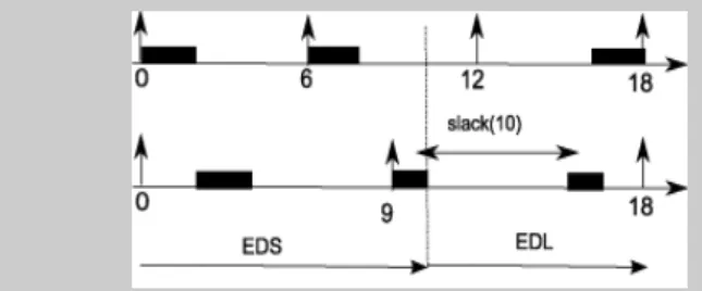
2.3 Simple example

To illustrate the analysis presented, we provide a simple example which consists of two periodic tasks J1(2, 6, 6) and

J2(2, 9, 9). We note that the hyperperiod equals 18 and the

Fig. 1. The EDS schedule

Fig. 2. The EDL schedule

processor utilization is 5₉. If a uniprocessor system solely supports these two periodic tasks, EDF produces a valid schedule during the lifetime of the system and this schedule repeats cyclically every 18 time units (see figures 1 and 2). We observe that ΩEDS

T (0, 8) = 2 and ΩEDLT (0, 8) = 5.

Now, suppose that the periodic tasks are scheduled accord-ing to EDS from 0 to 10. To compute the slack at time 10, the EDL schedule is mapped out from 10 up to the end of the hyperperiod at time 18. And this enables us to deduce that δ(10) = 5 (see figure 3).

3. SLACK OF A PERIODIC TASK SET

In this section, we address the problem of determining the slack time of a periodic task set at time t, denoted as δ(t) and defined as the maximal continuous time the processor could be let idle or process additional tasks without jeopardizing the timing constraints of the periodic task set. First, let us compute the length of the slack at time 0, δ(0), obtained by applying EDL to T at time 0. Let xj = Tj− Dj for j=1 to n. Proposition 1 provides us

a formula to compute δ(0). Proposition 1.

δ(0) = min

k∈K{k − h(k)} (2)

Proof: Consider the schedule produced by EDL for T from 0 to P. Let k be the first instant between 0 and P such that there is no idle time within [0 + δ(0), k] and all the tasks with a deadline greater than k are entirely processed within [k, P]. It follows that δ(0) is equal to the length of the time interval [0, k] minus the total quantity of processor time assigned to the requests with a deadline less than or equal to k. All the requests of every task Jj whose

ready time is greater than k + xj must then be rejected. It

follows that δ(0) = k −h(k). Let t be any time instant in K and α(t) = t − h(t). Let us prove that ∀t 6= k, α(t) ≥ δ(0).

Case 1: t < k. From definition of k, we know that some requests with a deadline posterior to t can be processed within [0, t]. Let Q(t) be the processor time reserved to these tasks. It follows that δ(0) = α(t) − Q(t) and conse-quently δ(0) < α(t).

Case 2: t > k and there may exist some requests with a deadline posterior to t which are processed within [0 + δ(0), t]. Then, δ(0) = α(t) − Q(t) − ϕ(t) where ϕ(t) denotes the total idle time within [0+δ(0), t]. Consequently, δ(0) <

(5)

Fig. 3. Slack at time 10

α(t). Finally, it follows that δ(0) = min{α(t); t ∈ K} which corresponds to (2).2

Example:

Consider the previous periodic task set. For every task Jj

in the set, we have xj = 0. Through formula 2, we obtain

δ(0) = min(4, 5, 6, 8) i.e. 4, which represents the length of the first idle time interval in the EDL schedule produced at time 0 (see figure 2).

We now show a lemma which will serve to derive a lower bound to the slack at any time.

lemma 1. For any release time e that coincides with the end of an idle time interval, δ(e) ≥ δ(0)

Proof: At time e, all the available tasks released before e have been processed since the processor is idle just before e by hypothesis. Consider the set of requests available from time e to time P and form the associated set of aperiodic tasks. Let S be this set and consider time e as a new time zero. From theorem 1, applying EDL to S from e will produce a schedule where the total idle time that follows e is maximized and corresponds to the slack, δ(e) . Now, we show that δ(0) provides a lower bound to the length of this idle time. For this purpose, let t be the first deadline after e such that t is followed by an idle time interval and the processor is fully utilized between e + δ(e) and t. Assume that time t coincides with the deadline of a request, for every task in T . In particular, t coincides with the deadline of the request that is released at time e. Let Jl be this task. Then, ∃k, k0 ∈ N such that

e = kTl and t = k0Tl− xl. This assumption takes care of

the worst possible case in the sense that the processor is required to provide maximum service in the time interval [kTl, k0Tl− xl]. Let ζ = (k0 − k)Tl− xl.It follows that

δ(e) ≥ ζ − h(ζ). Since ζ ∈ K, proposition 1 enables us to conclude that δ(e) ≥ δ(0).2

We are now prepared to provide a safe lower bound on the available slack at any time instant.

Theorem 2. For any time t, δ(t) ≥ δ(0)

Proof: Without loss of generality, we assume that t ∈ {0, 1, 2, ..., P} since the schedule is periodic, and conse-quently δ(t) = δ(t + kP), k = 1, 2, . . . The theorem is proved by induction on the units of time t. The basis of induction corresponds to t = 0.

To carry out the induction step, we assume that the theorem is true at t i.e δ(t) ≥ δ(0) and prove that δ(t + 1) ≥ δ(0). Introduce Γ(t) to be the schedule produced by EDS from 0 to t and by EDL from t to P on T . δ(t) is then given by the length of the idle time that follows time t in Γ(t). Now, consider the schedule Γ(t + 1) and examine three cases.

Case 1: The processor is not occupied in [t, t + 1]. The processor will remain idle until the next release time. Let ei

be this time instant. It follows that δ(t + 1) = ei− t + δ(ei).

Since δ(ei) ≥ δ(0) from lemma 1, we have δ(t + 1) ≥ δ(0).

Case 2: The processor is processing, in [t, t + 1], a task J with deadline d and there is no task with a deadline less than or equal to d that is not yet completed at t.

As tasks are scheduled according to Earliest Deadline, J has the earliest deadline among the ready tasks at t. This implies that J is the first one to be scheduled after t in Γ(t).

We have to examine two subcases:

Subcase 2.1: Task J completes at t + 1 and there is an idle time starting at d in Γ(t) with a length equal to ∆, ∆ > 0. Consequently, J is scheduled between d − 1 and d in Γ(t). It follows that δ(t + 1) = δ(t) + ∆. Then, δ(t + 1) > δ(t) and consequently δ(t + 1) ≥ δ(0).

Subcase 2.2: Else. Γ(t + 1) is obtained from Γ(t) by a permutation of the idle time between t and t + 1 and the busy time for J between t + δ(t) and t + δ(t) + 1. Then, δ(t) = δ(t + 1) and consequently δ(t + 1) ≥ δ(0).

Case 3: The processor is processing, in [t, t + 1], a task J with deadline d and there is at least one task with a deadline less than d that is not yet completed at t. Let Ji

be the first released task that verifies this condition. Let ei and di be the release time and the deadline of Ji

that necessarily verifies ei > t since tasks are scheduled

according to Earliest Deadline first. We have to examine two subcases:

Subcase 3.1: J is totally scheduled after di in Γ(t).

Conse-quently, J is not scheduled between ei and di in Γ(ei). As

there is no ready task with a deadline less than d which is uncompleted at t, there is no task scheduled within [t+1, ei] and so, δ(t+1) = δ(ei)+(ei−(t+1)) which implies

that δ(t + 1) ≥ δ(ei). Since δ(ei) ≥ δ(0) from Lemma 1,

then δ(t + 1) ≥ δ(0).

Subcase 3.2: J is partially scheduled before di in Γ(t). As

J is scheduled after Ji in [ei, di] since d ≥ di, Γ(t + 1)

is obtained from Γ(t) by a permutation of the idle time between t and t + 1 and the busy time for Ji between

t + δ(t) and t + δ(t) + 1. It follows that δ(t + 1) = δ(t) and consequently δ(t + 1) ≥ δ(0).2

Theorem 2 says that the slack of a periodic task set is never less than its slack at time 0. Furthermore, the demonstration enables us to state that the slack has local maximum at the beginning of every idle time interval, is linear decreasing within any idle time interval, and is non

(6)

40 pt 0.556 in 14.1 mm 40 pt 0.556 in 14.1 mm

Fig. 4. Fluctuations in slack over time increasing in any busy time interval.

Example:

Figure 4 depicts variations in the slack within the first hyperperiod [0, 18] for the periodic task set of the previous example. It illustrates both results of lemma 1 and theorem 2, i.e the slack is never less than δ(0), here equal to 4.

4. SLACK UNDER DELAYED-SCHEDULE CONSIDERATIONS

Consider once again a periodic task set T scheduled ac-cording to EDS up to current time τ . Assume that the slack was consumed partialy while preserving the deadlines and the periodic tasks have been held up between 0 and τ . For example, this can be due to the on-line admission of aperiodic tasks or processor shutdowns. We are interested to assess the impact of periodic task postponement upon slack variations. We establish the following theorem: Theorem 3. For any time t ≥ τ , δ(t + 1) ≥ min(δ(t), δ(0)).

Proof: Let us denote by Ψ(t) the schedule produced by EDS from 0 to t, t ≥ τ and by EDL from t to P. And let Γ(t) be defined as previously, i.e without no periodic task postponement. We pick up the three cases of theorem 2.

Case 1: The processor is not occupied between t and t + 1 in Ψ(t + 1). Ψ(t + 1) from time t + 1 is necessarily identical to Γ(t + 1) because all the tasks which are completed at t + 1 in Ψ(t + 1) are also completed in Γ(t + 1). From theorem 2, we deduce that δ(t + 1) ≥ δ(0).

Case 2: The processor is processing, in [t, t + 1], a task J with deadline d and there is no task with a deadline less than or equal to d that is not yet completed at t. As tasks are scheduled according to Earliest Deadline First, J has the earliest deadline among the ready tasks at t. This implies that J is the first one to be scheduled after t in Ψ(t).

We have to examine two subcases:

Subcase 2.1: Task J completes at t + 1 and there is an idle time starting at d in Ψ(t) with a length equal to ∆, ∆ > 0. Consequently, J is scheduled between d − 1 and d in Ψ(t). It follows that δ(t + 1) = δ(t) + ∆. Then, δ(t + 1) > δ(t) which implies that δ(t + 1) ≥ δ(t).

Subcase 2.2: Else. Ψ(t + 1) is obtained from Ψ(t) by a permutation of the idle time between t and t + 1 and the busy time for J between t + δ(t) and t + δ(t) + 1. Then, δ(t) = δ(t + 1) which implies that δ(t + 1) ≥ δ(t).

Case 3: The processor is processing, in [t, t + 1], a task J with deadline d and there is at least one task with a deadline less than d that is not yet completed at t. Let Ji

be the first released task that verifies this condition. Let ei and di be the release time and the deadline of Ji that

necessarily verifies ei ≥ t + 1 since tasks are scheduled

according to Earliest Deadline first. We have to examine two subcases:

Subcase 3.1: J is totally scheduled after di in Ψ(t). Let us

prove that such a situation may occur only if δ(t) > δ(0). Ψ(t + 1) is obtained from Ψ(t) by a permutation of the idle time between t and t + 1 and the busy time for J at a time instant greater than di. Consequently, δ(t + 1) = δ(t) − 1.

There is no ready task with a deadline less than d and uncompleted execution at time t. Consequently all the schedules Ψ(t0) and Γ(t0) with t ≤ t0 ≤ di restricted

to [t0, di] are identical. It follows from theorem 2, that

δ(t0_{) ≥ ∆(0) and in particular δ(t + 1) ≥ ∆(0). As δ(t +}

1) = δ(t) − 1, it results that neccessarily, δ(t) > δ(0) and δ(t + 1) ≥ δ(0).

Subcase 3.2: J is partially scheduled before di in Ψ(t). As

J is scheduled after Ji in [ei, di] since d ≥ di, Ψ(t + 1)

is obtained from Ψ(t) by a permutation of the idle time between t and t + 1 and the busy time for Ji between

t + δ(t) and t + δ(t) + 1. It follows that δ(t + 1) = δ(t) and then δ(t + 1 ≥ δ(t).2

Theorem 3 says that, if at a given time instant, the slack is greater than or equal to δ(0), even though periodic tasks have been postponed, the slack will never decrease below δ(0). Furthermore, if at a given time instant, the slack is less than δ(0), then it will grow up δ(0) without any decreasing phase.

Such results allow us to reduce the computational com-plexity of the on-line guarantee routine to 0(1) when deadling with the problem of the on-line acceptance of aperiodic tasks or temporary processor shutdown. This is done by keeping trace of a lower bound to the slack, then avoiding to compute the exact value, as seen in the following example.

Example:

Consider the previous periodic task set and assume that one nonpreemptable aperiodic task arrives at time 5 and another one at time 8, both with execution time equal to 2 (see figure 5). From theorem 2, the slack at time 5 is surely no less than δ(0), i.e. 4 which guarantees the feasible immediate execution of the first aperiodic task together with the periodic tasks without requiring computation of the exact value of the slack, here equal to 5. Consequently, a lower bound on the slack at the finishing time of the first aperiodic task is clearly 3.

Theorem 3 guarantees that the slack will never be less than 3 after time 5 (see figure 6). At time 8, the second aperiodic task may be executed without needing exact slack computation since its execution time is less than the lower bound on the slack. When the aperiodic task terminates at time 10, a new lower bound is consequently 1.

Figure 6 enables us to show the non decreasing variation of the slack until it will become greater than or equal to

(7)

Fig. 5. Scheduling periodic and nonpreemptable aperiodic tasks

Fig. 6. Fluctuations in slack over time 4.

Now, we prove that the slack at time 0 of a given syn-chronous periodic task set gives a lower bound on the slack of this periodic task set for any release time scenario. Theorem 4. The slack δ(0) obtained at time 0 is valid for any release time scenario.

Proof: Let hAsyn(t) be the demand bound function ob-tained for any asynchronous release time scenario. From its definition, we have: hAsyn(t) ≤ h(t). It follows that ∀t ≥ 0, t − hAsyn_{(t) ≥ t − h(t) ≥ δ(0). It follows that}

mint≥0(t − hAsyn(t)) ≥ δ(0). Hence, δ(0) is the minimum

slack valid for any release time scenario.2 5. SUMMARY

The most important property of a hard real-time system is not high speed, but predictability. The deterministic behavior of a system typically depends on the scheduler. Although interrupts handling and processor shutdown may improve the performance in terms of energy saving or quality of service, they have major influence on periodic task execution. A trustworthy timing guarantee of system behavior is then needed at every moment for avoiding over-load situations which result in deadline misses. These ones are mainly due to unpredictable aperiodic tasks as well as processor shutdown for dynamic power management with insertion of sleeping modes. Timing guarantee has to be achieved with appropriate and efficient on-line kernel mechanisms which lead to compute the slack at run-time. In this paper, we described theoretical results from the analysis of the Earliest Deadline schedule for a set of periodic tasks. First, theorem 2 expresses us that a safe lower bound on the available slack in the absence of task postponement is the slack at time zero than can be ob-tained by an off-line computation in pseudo-polynomial time.

In previous studies, the author showed that the overhead

in computing the exact value of slack at run-time becomes serious as the number of tasks increases. Consequently, we were interested in providing a way to significantly reduce the overhead. Then theorem 3 gives us properties on the Earliest Deadline schedule when authorizing periodic task postponement. Predictability on the schedule is attained by a precise knowledge on slack variations over time. Through an example, we illustrated how such theoreti-cal results can be useful. We can develop either an on-line sufficient schedulability condition based on slack ap-proximation in O(1) or an exact schedulability test that prevents from unecessary and costly computations. This permits to reduce the overhead incurred by the scheduler in terms of both time and energy consumption which is highly desirable in battery powered computers.

The work presented in this paper assumed that all the tasks were independent with no energy limitation. It will be challenging to develop a similar scheduling analysis to handle other cases such as when tasks experience blocking due to resource sharing or when the ED-H algorithm serves to schedule the tasks with energy harvesting constraints (25).

REFERENCES

[1] J. Stankovic, K. Ramamritham, Tutorial Hard Real-Time Systems, Computer Society Press of the IEEE, (1988).

[2] P. Balbastre, I. Ripoll, A. Crespo, Minimum Deadline Calculation for Periodic Real-Time Tasks in Dynamic Priority Systems, IEEE Transactions on Computers, (2007)

[3] P. Balbastre, I. Ripoll, A. Crespo, Analysis of window-constrained execution time systems, Real-Time Systems (2007).

[4] P. Balbastre, I. Ripoll, A. Crespo, Period sensitivity analysis and D–P domain feasibility region in dynamic priority systems, Journal of Systems and Software, (2009).

[5] E. Bini, M. Di Natale and G. Buttazzo, Sensitivity Analysis for Fixed-Priority Time Systems, Real-Time Systems, 39 (1-3) (2008) 5–30.

[6] L. Bougueroua, L. George, S. Midonnet, Dealing with execution-overruns to improve the temporal robustness of real-time systems scheduled FP and EDF, Proceed-ings of the Second International Conference on Systems (2007).

[7] J. P. Lehoczky, S. Ramos-Thuel, An optimal algorithm for scheduling soft-aperiodic tasks fixed priority preemp-tive systems, Proceedings of the 13th IEEE Real-Time Systems Symposium (1992) 110-123.

[8] R. I. Davis, On Exploiting Spare Capacity in Hard Real-Time Systems, PhD thesis, University of York, (1995).

[9] G. Buttazzo, Achieving scalability in real-time sys-tems, IEEE Computer 39 (5) (2006) 54-59.

[10] X. Zhong, C.Z. Xu, System-wide energy minimization for real-time tasks: lower bound and approximation, Proceedings of the IEEE/ACM international conference on Computer-aided design (2006) 516–521.

[11] G.C. Buttazzo, Hard real-time computing systems, Springer (2005).

[12] M.L. Dertouzos, Control robotics: The procedural control of physical processes, Proceedings of IFIP

(8)

40 pt 0.556 in 14.1 mm 40 pt 0.556 in 14.1 mm Congress (1974) 807–813.

[13] M. Chetto, A. Queudet, A Note on EDF Scheduling for Real-Time Energy Harvesting Systems, IEEE Trans-actions on Computers 63(4) (2014) 1037–1040.

[14] C.L. Liu, J.W. Layland, Scheduling algorithms for multiprogramming in a hard-real-time environment, J.ACM 20 (1) (1973) 46–61.

[15] S. K.Baruah, R. R. Howell, and L. E. Rosier, Al-gorithms and Complexity Concerning the Preemptive Scheduling of Periodic Real-Time Tasks on One Proces-sor, Real-Time Systems 2 (4) (1990) 301–324.

[16] A. Guasque, P. Balbastre, and A. Crespo, Real-time hierarchical systems with arbitrary scheduling at global level. J. Syst. Softw. 119, (September 2016), 70–86. DOI:https://doi.org/10.1016/j.jss.2016.05.040.

[17] S. K. Baruah, A. K. Mok, and L. E. Rosier, Pre-emptively scheduling hard real-time sporadic tasks on one processor. In Proceedings 11th Real-Time Systems Symposium, pages 182–190 (1990).

[18] S. K. Baruah, R. R. Howell, and L. E. Rosier, Fea-sibility problems for recurring tasks on one processor. Theor. Comput. Sci., 118:3–20 (1993).

[19] I. Ripoll, A. Crespo, and A. K. Mok, Improvement in feasibility testing for real-time tasks. Real-Time Syst., 11(1):19–39 (1996).

[20] M. Spuri, Analysis of deadline scheduled real-time systems. Technical report, (1996).

[21] G. Buttazzo, Rate Monotonic vs. EDF: Judgment Day, Real-Time Systems 29(1) (2005) 5–26.

[22] J.Y.K. Leung, M.L. Merril, A note on preemptive scheduling of periodic real-time tasks, Information Pro-cessing Letters 20 (30) (1980) 115–118.

[23] H. Chetto, M.Chetto, Some Results of the Earliest Deadline Scheduling Algorithm, IEEE Transactions on Software Engineering 15 (10) (1989) 1261–1269. [24] M. Chetto-Silly, The EDL server for scheduling

peri-odic and soft aperiperi-odic tasks with resource constraints, Real-Time Systems 17 (1) (1999) 1–25.

[25] M. Chetto, Optimal Scheduling for Real-Time Jobs in Energy Harvesting Computing Systems, IEEE Transac-tions on Emerging Topics 2 (2) (2014) 122–133.