HAL Id: hal-01228454
https://hal.archives-ouvertes.fr/hal-01228454
Preprint submitted on 13 Nov 2015
HAL is a multi-disciplinary open access archive for the deposit and dissemination of sci-entific research documents, whether they are pub-lished or not. The documents may come from teaching and research institutions in France or abroad, or from public or private research centers.
L’archive ouverte pluridisciplinaire HAL, est destinée au dépôt et à la diffusion de documents scientifiques de niveau recherche, publiés ou non, émanant des établissements d’enseignement et de recherche français ou étrangers, des laboratoires publics ou privés.
Does Activating Sick-Listed Workers Work? Evidence
from a Randomized Experiment
Kai Rehwald, Michael Rosholm, Bénédicte Rouland
To cite this version:
Kai Rehwald, Michael Rosholm, Bénédicte Rouland. Does Activating Sick-Listed Workers Work? Evidence from a Randomized Experiment. 2015. �hal-01228454�
Dale Squires
EA 4272
Does Activating Sick-Listed Workers
Work?
Evidence from a Randomized Experiment
Kai Rehwald*
Michael Rosholm*
Bénédicte Rouland**
2015/25
(*) Aarhus University (**) LEMNA, Université de Nantes
Laboratoire d’Economie et de Management Nantes-Atlantique Université de Nantes
Chemin de la Censive du Tertre – BP 52231 44322 Nantes cedex 3 – France www.univ-nantes.fr/iemn-iae/recherche
D
o
cu
m
en
t
d
e
T
ra
va
il
W
o
rk
in
g
P
ap
er
Does Activating Sick-Listed Workers Work? Evidence from a
Randomized Experiment
Kai REHWALD∗ Michael ROSHOLM† Bénédicte ROULAND‡§
This version: November 2015
Abstract
Using data from a large-scale randomized controlled trial conducted in Danish job centers, this paper investigates the effects of an intensification of mandatory return-to-work activities on the subsequent labor market outcomes for sick-listed workers. Using variations in local treatment strategies, both between job centers and between randomly assigned treatment and control groups within a given job center, we compare the relative effectiveness of alternative interventions. Our results show that the use of partial sick leave increases the length of time spent in regular employment and non-reliance on benefits, and also reduces the time spent in unemployment. Traditional active labor market programs and the use of paramedical care appear to have no effect at all, or even an adverse effect.
JEL Classification: J68, C93, I18
Keywords: Long-term Sickness; Vocational Rehabilitation; Treatment Effects;
Random-ized Controlled Trial
1
Introduction
As highlighted in the OECD (2010) report on Sickness, Disability and Work, sickness policy is rapidly moving to center stage in the economic policy agenda of most OECD countries. Bud-getary considerations are one of the key reasons for this. Expenditure on paid sick leave in OECD
∗K. Rehwald ([email protected]): Department of Economics and Business Economics, Aarhus University †M. Rosholm ([email protected]): Department of Economics and Business Economics, Aarhus University ‡B. Rouland ([email protected]): LEMNA-TEPP, University of Nantes. Correspondence to:
Bénédicte Rouland, Université de Nantes IEMN-IAE, Chemin de la Censive du Tertre, BP 52231, 44322 Nantes Cedex 3, France.
§We would like to thank Knut Røed as well as seminar participants at CREST (Paris), IFAU (Uppsala), the
University of Nantes, IZA (Bonn) and SFI (Copenhagen), and participants at the 2013 TEPP Conference “Re-search in Health and Labour”, the 2013 DGPE Workshop, the 2013 Annual Workshop of the Centre for Re“Re-search in Active Labour Market Policy Effects (CAFÉ), the 2014 Annual Meeting of the Society of Labor Economists (SOLE), the 9th Nordic Summer Institute in Labour Economics, the “Empirical Strategies” Mini-Workshop in Bergen, the 2014 Annual Conference of the European Economic Association (EEA) and the 2015 Journées Louis-André Gérard-Varet in Public Economics, for their helpful comments and discussions. We gratefully acknowledge the financial and material support provided by the Danish Labor Market Authority. All remaining errors and shortcomings of the article are our own.
countries amounted on average to 0.8 percent of GDP in 2007.1 Although this figure might seem rather low, it is nevertheless a matter of great concern in the current context of growing public deficits and debt burdens. In comparison, public spending on unemployment benefits reached “only” 0.55 percent of GDP in the same year.2 Furthermore, absence due to sickness also implies a reduced labor supply, lost production, and health-related costs.3
Beyond the financial aspect of paid sick leave, the reintegration of sick-listed workers into the labor market is also a matter of great concern. Empirical research on the labor market has shown that frequent and/or long-term spells of absence are associated with a higher risk of unemployment (Hesselius, 2007), and can significantly reduce a worker’s subsequent earnings or prospect of employment(Markussen, 2012). The probability that a worker will then become inactive and dependent on a permanent disability pension also increases.
The importance of well conceived sickness policies is clear in this context. Such policies are essential both for the sick-listed worker (in terms of his/her successful reintegration) and for society as a whole (in view of budgetary constraints). Sickness policies have recently shifted from being passive towards a more employment-orientated approach, aiming both at reducing benefit dependency and increasing rates of employment.4 Taking Denmark as an example, vocational
rehabilitation measures were implemented in 16 percent of all periods of sickness benefit in the years 2009-2011, compared to only seven percent in the period 2005-2007 (Boll et al., 2010). Vocational rehabilitation includes traditional active labor market programs (e.g., internships), paramedical care (e.g., physical therapy), and graded return-to-work (partial sick leave).
Our aim in this paper is twofold. First, we wish to assess the effects of an intensification of return-to-work activities on sick-listed workers’ subsequent labor market outcomes. Second, we aim to compare the relative effectiveness of the alternative interventions. Specifically, we use results from a large-scale randomized controlled experiment conducted in Danish job centers in 2009 among newly registered sick-listed workers. The treatment lasted four months and consisted of a combination of weekly meetings with caseworkers and intensive mandatory return-to-work activities in the form of graded return-to-work (partial sick leave), traditional activation, and/or paramedical care.
Our empirical strategy and key results can be summarized as follows. We first rely on a simple difference-in-means approach to identify the causal effect of offering a more intensive treatment package on the subsequent labor market outcomes for newly sick-listed workers. Specifically,
1OECD data on social expenditure, taken from the OECD (2010) report on Sickness, Disability and Work.
The term ’sickness’ refers to public and mandatory private paid sick leave programs (occupational injury and other sickness-related daily allowances).
2
OECD data on Labour Market Programmes, extracted from OECD data bank (http://stats.oecd.org/). As for Denmark—the country under consideration in this paper—expenditure on paid sick leave amounted to 1.4 percent, while public spending on unemployment benefit reached 0.96 percent of GDP in 2007.
3
According to the Danish Ministry of Employment, absence due to sickness (short and long term) in 2006 reduced the supply of labor by five percent, which implies a cost of more than two percent of GDP.
4
we estimate a causal intention-to-treat effect on four outcome variables: accumulated weeks in regular employment, self-sufficiency (i.e., all forms of non-reliance on benefits), sickness, and unemployment. Second, in the spirit of Markussen and Røed (2014), we exploit variation in local treatment strategies, both between job centers and between treatment and control groups within a given job center, to compare the relative effectiveness of the alternative measures used. Our findings reveal firstly that the experimental intervention as a whole has been ineffective. Sick-listed workers initially assigned to the treatment group spent less time in regular employment and self-sufficiency than their peers in the control group. Nevertheless, our results also show that a greater emphasis on offering graded return-to-work programs is associated with an increase in regular employment and self-sufficiency, and lower unemployment. On the other hand, traditional activation and paramedical care appear to have either no impact at all, or even an adverse impact. Taken in the round, our results suggest that programs focusing on graded return-to-work are the most effective in improving sick-listed workers’ subsequent labor outcomes. These programs are associated with strong and long-lasting effects, but only for workers sick-listed from regular employment and for those with physical (non-mental) disorders.
In line with the rich literature on the effectiveness of active labor market policies for unem-ployed workers (see Card et al. (2010) for a meta-analysis), our study relates to the expanding literature on the impacts of return-to-work policies for (long-term) sick-listed workers.5 Return-to-work can be associated with various forms of interventions, including workplace-based6, edu-cational, medical, and social interventions. The results are mixed, however; Frölich et al. (2004) for example, found that rehabilitation programs for the long-term sick (more than four weeks) in Sweden had no favorable effects at all, but that workplace interventions were less damaging than the alternative strategies. In a randomized study of the inflow of Swedish sick-listed individuals, Engström et al. (2015) found some negative effects associated with having early meetings to assess individuals’ work capacity (more sickness absence and a higher probability of receiving disability benefits). In contrast, Everhardt and de Jong (2011) found strong positive impacts of return-to-work activities for long-term (nine months) sick employees in the Netherlands in terms of their likelihood of returning to work.
Some of the literature on workplace-based interventions focuses specifically on the effects of graded return-to work programs, i.e., some combination of part-time work and sickness benefits.7
5
There is also another branch of the literature that relates to the impacts of return-to-work policies for tem-porary disabled workers. See for instance Aakvik et al. (2005) and Markussen and Røed (2014) for a study of the Norwegian Vocational Rehabilitation program. While there is no absolute definition of long-term sick leave, workers typically call on a temporary disability insurance system following a period of sick pay (which is more generous than the disability insurance); however this is available only for a limited period of time (usually around one year).
6Reviewing recent medical research, Van Oostrom et al. (2009) concluded that workplace interventions are
effective in reducing sickness absence among workers with musculoskeletal disorders compared with normal forms of care, although they are not effective in improving health outcomes.
7
While accurate and reliable evidence remains scarce, Markussen et al. (2012) provides an excep-tion. Using data collected from Norwegian administrative registers, the authors concluded that the use of graded (partial) rather than non-graded (full) sickness absence certificates reduces the length of periods of absence, and significantly improves the propensity for employment in subsequent years. Andrén and Svensson (2012) found that Swedish employees with musculoskele-tal disorders assigned to part-time sick leave were more likely to recover to full work capacity than those assigned to full-time sick leave. From a randomized controlled trial performed in Finland among 63 patients with musculoskeletal disorders, Viikari-Juntura et al. (2012) showed that part-time sick leave reduced both the time taken to return to regular duties and the amount of sickness absence in the one-year follow-up period. In the Danish graded return-to-work pro-gram, Høgelund et al. (2010) found that participation in such a program significantly increased the probability that sick-listed workers returned to regular working hours. However, Nielsen et al. (2014) showed that its effect on the return to self-support differed substantially among the municipalities, and therefore warned against generalizing the results of the study to other Danish municipalities. Moreover, Høgelund et al. (2012) found no impact of the Danish graded return-to-work program for workers with mental health problems.
Based on a large-scale experimental design, the present study adds to the existing literature by offering a comprehensive evaluation of intensive mandatory return-to-work activities (activation requirements). In particular, we focus not only on workplace-based interventions but also on paramedical care, and thus compare the relative effectiveness of alternative intensive interventions (traditional activation vs. paramedical care vs. partial sick leave). We also consider all kind of diseases rather than focusing on a specific subsample of sick-listed workers as others have done. The rest of the paper is organized as follows. Section 2 includes details of the randomized experiment. Section 3 is a description of the data and variables. Section 4 provides an explanation of the empirical strategy, and section 5 contains the findings. Some conclusions are given in Section 6.
2
The randomized experiment
The Danish sick-leave policy In Denmark, all employees, all self-employed, and all indi-viduals receiving unemployment insurance benefits are entitled to receive compensation for each day they cannot work due to sickness (whether the sickness is work-related or not), provided they have worked at least 120 hours within the thirteen successive weeks prior to their sickness absence. Although the benefit period can be extended to more than a year under certain
spe-Finland. The authorities have strongly promoted the use of these in recommending partial sick leave as the mechanism of choice, where sick leave is needed. See Kausto et al. (2008) for a review of the use of partial sick leaves in the Nordic countries. A similar arrangement has also been in place in the UK since 2010 (known here as the “Fit Note”).
cific conditions, sickness benefits are normally available for a maximum of 52 weeks within an eighteen-month period. The employer finances the first 21 days of the sickness absence8, while municipalities are then responsible for funding the remaining period.
The municipalities play a key role in the return-to-work process. Besides managing sickness absence and work rehabilitation, it is their responsibility to monitor and assess recipients of sickness benefits. More precisely, municipalities must conduct an assessment of all sickness benefit cases no later than the eighth week of the sickness absence, and every fourth week from then on (or every eighth week in less complicated cases). Follow-up assessments must rely on updated and coordinated medical, social, and vocational information. The aim of these mandatory follow-up interviews is first to verify that the sick-listed individual is actually eligible for the benefit (i.e., s(he) has a work incapacity) and second, to help him or her to return to work as quickly as possible. Municipal case managers can implement various vocational rehabilitation measures, from job counselling to wage-subsidized job training and professional courses, and including graded return-to-work (partial sick leave).
It is worth noting that municipalities have economic incentives to reintroduce sick-listed individuals to the workplace because the state reimburses their expenditure on sickness benefit to varying degrees, depending on whether any return-to-work activities are implemented or not. Municipalities also have an incentive both to reduce expenditure on sickness benefit because the entitlement to reimbursement only applies to cases lasting less than 52 weeks, and to use part-time (rather than full-time) sick-listing, because this also reduces the final burden on them. Finally, if despite medical treatment and vocational rehabilitation the sick-listed worker is unable to return to ordinary employment, the municipality may refer him or her to a permanent wage-subsidized job (fleksjob) with reduced working hours and special tasks. To be eligible for a
fleksjob, the sick-listed worker must have a permanently reduced work capacity of at least 50
per-cent and be no older than 65. The main difference between a fleksjob and graded return-to-work is that subsidized employment in a fleksjob is granted for an unlimited time while participation in a graded return-to-work program is always temporary. If the sick-listed individual cannot return to a fleksjob, the municipality may award disability benefits.
The experiment In early 2009, the National Labor Market Authority in Denmark launched a randomized controlled trial (hereafter RCT) to test at a small scale some of the elements that were to be included in the forthcoming legislation on active interventions relating to those receiving sickness benefits.9 The overall purpose of this experiment was to examine whether sick-listed workers who behave in a more proactive way during their sickness period can achieve a
8At the time of the experiment (2009), the employer was required to finance the first fourteen days of the
illness period; the rules on this changed in October 2009.
9
A new and intensified treatment package was eventually rolled out nationally (with adjustments) in late 2009, when a new law governing the return-to-work of sick-listed workers was passed in Denmark.
greater degree of autonomy (in terms of returning to work and staying in work) than they would have done had they not behaved proactively. The present study is a report on the outcomes of this experiment.
The experiment was designed as an RCT conducted in 16 job centers across Denmark, with “random” assignment to treatment by birth year, even or odd. A total of 5,652 newly sick-listed workers were covered by the experiment, of which 2,795 were assigned to the control group and 2,857 to the treatment group.10 Individuals were notified that they had been assigned to the treatment group during the first follow-up meeting (no later than the eighth week of their sickness absence) by means of a standard letter from The National Labor Market Authority. Newly registered sick-listed workers born in odd years were subject to intensive efforts (treatment group), while those born in even years were subject to normal levels of effort (control group). Although assignment to treatment was predetermined, not random, we nevertheless consider our study to be an RCT; individuals were not made aware of the assignment mechanism, and a person’s birth year is “random” from his/her own perspective.
The treatment lasted 18 weeks and consisted of a combination of weekly meetings with caseworkers AND intensive mandatory return-to-work activities in the form of either a graded return-to-work (partial sick leave) and/or traditional activation and/or paramedical care. More precisely, traditional activation includes vocational guidance advice and courses aimed at enhanc-ing skills, together with internships and on-the-job trainenhanc-ing. Paramedical care consists of courses on handling one’s own situation, psychological consultations, nutritional counselling, and exercise including back exercises and other physical training. Lastly, the aim of the graded return-to-work measure is to support employees with reduced work ability to continue and return to work via partial sick leave. This involves working part-time (a reduction in working hours by at least four hours per week) and receiving a partial sickness benefit for the hours off work, on top of a partial salary (at a normal hourly rate). The underlying idea is that most sick leave days are a result of non-communicable diseases, and a person’s work capacity while sick may be reduced but it is not nothing. The return to regular working hours should take place as soon as possible, and certainly within the 52-weeks payment period of full sickness benefits. Graded return-to-work must be implemented with the agreement of the employer, the sick-listed worker, and the municipality. In practice, either the sick-listed worker and the employer arrange a graded return-to-work on their own initiative and then ask the municipality to approve this, or the municipality determines that the sick-listed worker is able to work part-time and therefore asks him or her to agree a graded return-to-work with the employer. If the sick-listed worker refuses to enrol in the program even though the municipal case manager recommends it, the sick benefit can be reduced.
10
Table A1 in the Appendix shows the number of individuals by employment region, job center and treatment status.
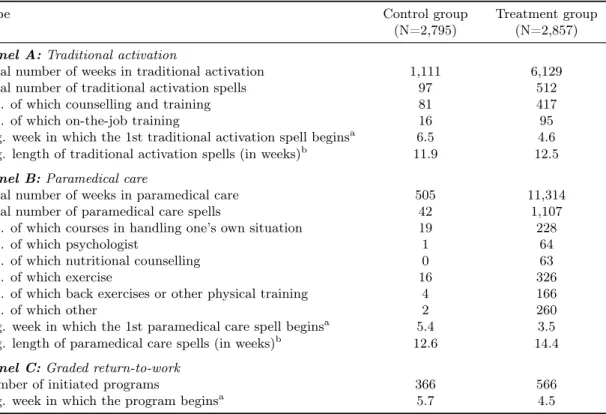
Within four weeks of the first interview, individuals in the treatment group were required to participate in some kind of program (graded return-to-work, traditional activation and/or paramedical care) for at least ten hours a week for up to four months. Table 1 provides details of the extent of these return-to-work activities. Compared with the control group, it is clear that the treatment group received more intensive programs of treatment. For treated individuals, the number of return-to-work activities (all three types) was higher, and the interventions generally began earlier and lasted longer.
Table 1: Number of return-to-work activities by type and treatment status
Type Control group
(N=2,795)
Treatment group (N=2,857)
Panel A: Traditional activation
Total number of weeks in traditional activation 1,111 6,129 Total number of traditional activation spells 97 512
... of which counselling and training 81 417 ... of which on-the-job training 16 95 Avg. week in which the 1st traditional activation spell beginsa 6.5 4.6 Avg. length of traditional activation spells (in weeks)b 11.9 12.5
Panel B: Paramedical care
Total number of weeks in paramedical care 505 11,314 Total number of paramedical care spells 42 1,107
... of which courses in handling one’s own situation 19 228
... of which psychologist 1 64
... of which nutritional counselling 0 63
... of which exercise 16 326
... of which back exercises or other physical training 4 166
... of which other 2 260
Avg. week in which the 1st paramedical care spell beginsa 5.4 3.5
Avg. length of paramedical care spells (in weeks)b 12.6 14.4
Panel C: Graded return-to-work
Number of initiated programs 366 566 Avg. week in which the program beginsa 5.7 4.5 a
Measured in weeks since first follow-up meeting with the municipal caseworker (typically eight weeks after the onset of illness).
b
When calculating the average length of activation spells in weeks, uninterrupted sequences of alternative activities are treated as a single spell (93 spells in the control and 492 spells in the treatment group). Similarly for the average length of paramedical care spells in weeks (40 spells in the control and 787 spells in the treatment group).
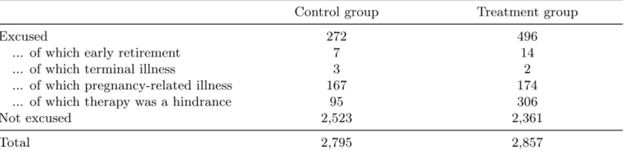
Moreover, the outcome from the first follow-up meeting with the municipal caseworker (eight weeks after the onset of illness) could also be a total program exemption for some sick-listed workers. As shown in Table 2, around 13 percent of all participants in the experiment were excused from any kind of return-to-work activity, mainly because therapy was a hindrance (52 percent of all cases of exemption), or because of a pregnancy-related illness (44 percent of cases). Exemption rates were higher in the treatment group (around 17 percent) than in the control group (almost ten percent). However, the exempted are still included in the analysis. Specifically, those exempted from the treatment group received the treatment as usual (i.e., the same as individuals in the control group) and are included in the treatment group. Those exempted from the control group also received the normal amount of return-to-work activity (even though they
were excused). We account for this significant number of “no-shows” by estimating intention-to-treat effects, so our results could be valid even given imperfect compliance.
Table 2: Number of individuals excused/not excused by reason and treatment status Control group Treatment group
Excused 272 496
... of which early retirement 7 14 ... of which terminal illness 3 2 ... of which pregnancy-related illness 167 174 ... of which therapy was a hindrance 95 306
Not excused 2,523 2,361
Total 2,795 2,857
Notes: The table shows the number of individuals excused/not excused by treatment status. The exempted are included in the analysis because exemption rates were higher in the treatment group than in the control group. Specifically, those exempted from the treatment group received the treatment as usual (i.e., the same as individuals in the control group) and are included in the treatment group. Those exempted from the control group also received the normal amount of return-to-work activity (even though they were excused).
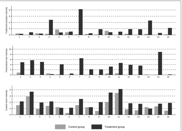
Finally, it is worth noting that the job centers were responsible for the organization of the experiment. They carried out interviews and decided on the composition and content of any vocational rehabilitation, accounting for the individuals’ needs and adapting to local conditions. Therefore, some variations in treatment intensity between job centers may be assumed. From Figure 1, it is very clear that there is substantial variation in the intensity of return-to-work activities, both between the 16 job centers covered by the experiment, and between treatment and control groups within a given job center.11 As we explain in Section 4, we exploit this variation in local treatment strategies to compare the effectiveness of the alternative return-to-work activities (graded return-to-return-to-work, traditional activation, and paramedical care).
3
Data and variables
The empirical analysis is based on four different data sets. First, we exploit unique Danish data derived from the controlled field experiment described above. These data include binary variables for each type of return-to-work activity (graded return, traditional activation and paramedical care) and for each meeting scheduled/held, as well as the number of hours per week in each type of activation and the timing of the intake. We can therefore follow participation accurately on a weekly basis. The data also include information about possible exemption from activation and the job center is identified in each case.
Second, from the DREAM register we obtained information about the type of social welfare benefit received in a given week12, and about individual characteristics. DREAM is an
amalga-11
Similarly, the overall management of the usual vocational rehabilitation is regulated by law, but the assessment and the implementation of individual cases are controlled at job center level. Therefore, there is also substantial variation in the intensity of return-to-work activities among the control group.
12
Figure 1: Traditional activation, paramedical care and graded return-to-work intensities by job center and treatment status 0 2 4 6 8
Traditional activation intensity
1 2 3 4 5 6 7 8 9 10 11 12 13 14 15 16 0 2 4 6 8 10
Paramedical care intensity
1 2 3 4 5 6 7 8 9 10 11 12 13 14 15 16 0 .1 .2 .3 .4
Graded return intensity
1 2 3 4 5 6 7 8 9 10 11 12 13 14 15 16
Control group Treatment group
Notes: Indices 1 to 16 on the horizontal axes refer to job centers: (1) Bornholm, (2) Gentofte, (3) Greve, (4) København, (5) Ringsted, (6) Vordingborg, (7) Aalborg, (8) Morsø, (9) Randers, (10) Holstebro, (11) Herning, (12) Horsens, (13) Svendborg, (14) Nyborg, (15) Odense and (16) Aabenraa. Traditional activation intensities are calculated as the average number of traditional activation weeks per individual in the first 20 weeks after enrolment. Similarly for paramedical care intensities. Graded return intensities are calculated as the proportion of individuals participating in a graded return-to-work program within the first 20 weeks.
mation of information from several different sources, and is updated once per month by the The National Labor Market Authority.13 Data from the DREAM register were obtained from the week in which the experiment began (i.e., between the first week of January 2009 and the third week of November 2009) up to the end of 2012, allowing a three-year follow-up. Specifically, we constructed four outcome variables from the DREAM database, using the weekly information on social transfer payments, namely the cumulative number of weeks spent in regular employment (i.e., employed), in non-reliance on benefits (i.e., self-sufficiency), in sickness and in unemploy-ment, where self-sufficiency covers the officially designated success criteria and covers all periods of non-benefit (self-sufficiency without employment, employment, and ordinary education).14
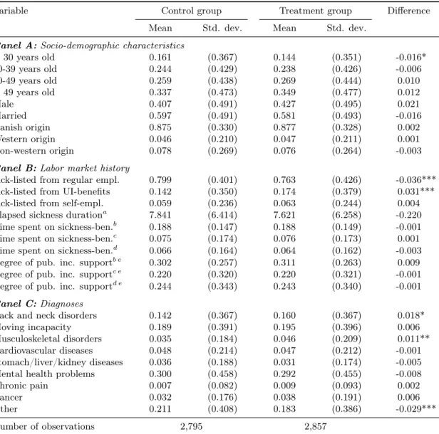
Besides the treatment package, our explanatory variables include age, gender, marital status, country of origin (three categories—Denmark, western, and non-western countries), the state before sickness (three categories—job, unemployment benefits and self-sufficiency), the duration of elapsed sickness at the start of the experiment, the proportion of time spent on sickness payments (in each of the three years before the sickness), and the same proportion for time spent on public income support of any kind (also in each of the three years before the sickness). Table 3, which shows means and standard deviations of the explanatory variables by treatment status, suggests that there are very few observed differences between the treatment and control groups.15 “Random” assignment based on birth year—even or odd—successfully balanced groups. The most significant difference, though nonetheless, relates to the status before sickness: the treatment group was on average in regular employment slightly less than the control group (76.3 vs. 79.9 percent), and in unemployment slightly more (17.4 against 14.2 percent).
Third, from Statistics Denmark we obtain data on socio-economic characteristics at the municipality level. In particular, for each municipality, we collected annual data on the total fertility rate, average age, and life expectancy for new born babies. We obtained quarterly information on the proportion of the working-age population with no more than ten years of schooling, on external and internal migration as a percentage of the population, and on the number of reported criminal offences per capita. As for the local labor market conditions, we calculated quarterly ratios as a percentage of the labor force for the working-age population outside the labor force, or receiving sickness benefits, or employed in the primary sector, as well
not receive social benefits in a given period, it is represented by empty week-variables.
13
The week-variables are only allowed to contain one type of compensation code at a time. This implies that the types of social benefits are ranked. The ranking implies that if a citizen changes the type of social benefit in the middle of a week, only the highest ranked type is registered that week.
14More precisely, we first generated indicators for regular employment, sickness, and unemployment using the
variable “status” from the DREAM register (i.e., the weekly information on labor market status). The outcome variable regular employment is defined using status 500 (i.e., the regular employment indicator is equal to one if the variable status is equal to 500). Similarly, the sickness indicator is based on statuses 890 to 899, while the unemployment indicator is generated from statuses 111, 112, 124, 125, 130 to 138, 200 to 300, and 730 to 738. Having defined these indicators, we computed the cumulative number of weeks spent in each state.
15
Table A2 in the Appendix shows the means and standard deviations of the explanatory variables by treatment status for the sample of 4,728 individuals (see later).
Table 3: Pre-treatment characteristics by treatment status (N=5,652)
Variable Control group Treatment group Difference Mean Std. dev. Mean Std. dev.
Panel A: Socio-demographic characteristics
< 30 years old 0.161 (0.367) 0.144 (0.351) -0.016* 30-39 years old 0.244 (0.429) 0.238 (0.426) -0.006 40-49 years old 0.259 (0.438) 0.269 (0.444) 0.010 > 49 years old 0.337 (0.473) 0.349 (0.477) 0.012 Male 0.407 (0.491) 0.427 (0.495) 0.021 Married 0.597 (0.491) 0.581 (0.493) -0.016 Danish origin 0.875 (0.330) 0.877 (0.328) 0.002 Western origin 0.046 (0.210) 0.047 (0.211) 0.001 Non-western origin 0.078 (0.269) 0.076 (0.264) -0.003
Panel B: Labor market history
Sick-listed from regular empl. 0.799 (0.401) 0.763 (0.426) -0.036*** Sick-listed from UI-benefits 0.142 (0.350) 0.174 (0.379) 0.031*** Sick-listed from self-empl. 0.059 (0.236) 0.063 (0.244) 0.004 Elapsed sickness durationa 7.841 (6.414) 7.621 (6.258) -0.220
Time spent on sickness-ben.b 0.188 (0.147) 0.188 (0.149) -0.001
Time spent on sickness-ben.c 0.075 (0.174) 0.076 (0.173) 0.001 Time spent on sickness-ben.d 0.066 (0.164) 0.064 (0.162) -0.003 Degree of pub. inc. supportb e 0.302 (0.257) 0.311 (0.263) 0.009
Degree of pub. inc. supportc e 0.220 (0.320) 0.220 (0.321) -0.001 Degree of pub. inc. supportd e 0.244 (0.343) 0.243 (0.340) -0.001
Panel C: Diagnoses
Back and neck disorders 0.142 (0.367) 0.160 (0.367) 0.018* Moving incapacity 0.189 (0.391) 0.195 (0.396) 0.006 Musculoskeletal disorders 0.035 (0.184) 0.046 (0.209) 0.011** Cardiovascular diseases 0.048 (0.214) 0.047 (0.212) -0.001 Stomach/liver/kidney diseases 0.036 (0.188) 0.031 (0.174) -0.005 Mental health problems 0.300 (0.458) 0.292 (0.455) -0.008 Chronic pain 0.007 (0.082) 0.009 (0.093) 0.002 Cancer 0.032 (0.176) 0.038 (0.191) 0.006 Other 0.211 (0.408) 0.183 (0.386) -0.029*** Number of observations 2,795 2,857
aat start of experiment (in weeks) bin year before sickness cin second last year before sickness din
third last year before sickness eany kind of public income support. Significance levels: * p < 0.10, ** p < 0.05, *** p < 0.01
as the number of full-time unemployed each quarter as a percentage of the labor force.
Finally, jobindex.dk is a collection of all the vacancies posted on the internet (online newspa-pers, job centers, job databases, etc.), which provides us with monthly information on the number of open vacancies and newly opened vacancies per unemployed person. We used this informa-tion to control for local environment characteristics when exploiting the variainforma-tion in treatment strategies across job centers.
4
Empirical strategy
4.1 The effect of the treatment bundle as a whole
Our first aim is to identify the overall causal effect of offering the intensified treatment package on sick-listed workers’ subsequent labor market outcomes. We may write
Yi = β0+ βZZi+ Xiβ + εi (1)
where Yi is the outcome of individual i (we consider four different measures, see below), Zi is a treatment status indicator equal to unity for clients assigned to the treatment group (zero otherwise), and Xi is the vector of pre-treatment characteristics summarized in Table 3 (with age entering linearly, not as a dummy-coded categorical predictor). Because treatment assignment is essentially random, Zi will, by design, be independent of Xi and of any other (observed or unobserved) pre-treatment variable.16 The coefficient βZ corresponds to the (conditional) difference in the means of outcome variable Yi between treated and controls. It identifies the
intention-to-treat (ITT) effect E(Yi|Zi = 1)− E(Yi|Zi = 0) if E(εi|Zi) = E(εi). This is likely to hold given that Zi is assigned at random. The experimental impact estimate bβZOLS can be interpreted causally; it is unbiased and consistent.
Regarding the dependent variable in equation (1), Yi, we consider four measures evaluated at different points in time: the number of weeks in (i) regular employment, (ii) self-sufficiency, (iii) sickness, and (iv) unemployment during the first, second, and third year after randomization.17 The self-sufficiency measure is meant to cover all forms of non-benefit receipt. It encompasses individuals in regular (i.e., wage) employment, as well as self-employed, housewives and everyone else not receiving public income transfers.18
Additionally, in order to trace the trajectory of treatment effects over time in greater de-tail, let Yi′ be an alternative set of response variables denoting the cumulative total number of
16
It immediately follows that conditioning on Xishould leave bβOLSZ unaffected. At the same time, we expect
a reduction in the residual variance to be accompanied by an increase in precision.
17
All individuals can be followed for 141 weeks, and outcome variables referring to the third year (up to 156 weeks) after enrolment are non-missing for all but eight individuals.
18
Exceptions are (subsidized) adult apprentices (“Voksenlærlinge”) and individuals receiving state educational support (“Statens Uddannelsesstøtte”). Both groups are considered to be self-sufficient.
weeks—running sums counting from the week of intake—in each of the four labor market statuses described above. We evaluate each of these outcomes at each week starting from the week of (individual) intake and ending with the 156th week after randomization (implying a total of 156 regressions per outcome variable). The results are presented graphically.
Besides its ease of use, the main advantage of the identification strategy discussed above is that it produces informative estimates even in the presence of imperfect compliance. Recall that there are a significant number of “no-shows”: more than one out of every six sick-listed workers assigned to treatment received treatment as usual (see Table 2). Under these conditions, the proposed experimental evaluation design (ITT) is the most relevant from a policy perspective. In fact, one of the aims of the experiment was to test the intensified treatment package on a small scale before it was eventually rolled out nationally with minor adjustments (impact pilot). The main drawback, however, is that a simple comparison of average labor market outcomes between treated and non-treated (“difference in means”) only allows us to evaluate the treatment package as a whole. Does the package work? While this question is relevant, it is clearly not the only causal relationship of interest. In particular, we would like to attribute the overall perfor-mance of the treatment bundle to its individual components (traditional activation, paramedical care, graded return-to-work). Yet, since the experiment was not designed as a multi-arm trial (the ideal experiment for answering this richer research question), isolating their individual im-pacts is a challenge. A naive comparison of those who did and those who did not participate in a particular treatment activity risks being biased by self-selection: observed differences in labor market outcomes are equal to the sum of the effect of the treatment on the treated and selection bias. Unbiased estimates can only be obtained if participation is as good as randomly assigned conditional on covariates (conditional independence)—a very strong assumption to make. In consequence, the “difference in means approach” does not enable us to compare the relative ef-fectiveness of the three alternative policies. Our second identification strategy, which is in spirit of that used by Markussen and Røed (2014), addresses this methodological challenge.
4.2 Disentangling the bundle, isolating effects
By exploiting variations in local treatment strategies, Markussen and Røed (2014) analyze the effectiveness of four alternative vocational rehabilitation programs for a large sample of temporary disability benefit recipients in Norway. We follow their approach.
To begin with, recall that there is substantial variation in treatment intensities both between the 16 job centers involved in the experiment and between the treatment and control groups within a given job center (Figure 1). As such, there are 32 distinct “local treatment environments”, each characterized by idiosyncratic working methods and treatment priorities. Differences in these “treatment cultures” may be seen in, e.g., the choice and combination of treatment types,
the speed with which newly registered clients are exposed to them, or the length of initiated activation spells. The resulting “treatment portfolio” is shaped by each of these choices, which may, in sum, be referred to as a “treatment strategy”. Our aim is to proxy these treatment strategies by vectors of local treatment strategy characteristics (φi). These can, in turn, be used
to identify the effects of alternative interventions.
The vectors of local treatment strategy characteristics (φi) are individual-specific and depend
on the treatment histories of all other sick-listed workers exposed to the same local treatment regime (more on this below). Each vector contains three elements—φSi (S=traditional acti-vation, paramedical care, graded return-to-work)—and is meant to describe “both the choice of (first) treatment, and the speed with which it is implemented” (Markussen and Røed, 2014: 15). We estimate the vector of local treatment strategy characteristics in the framework of a linear discrete transition rate model with competing risks. In particular, we consider exits from a single state (“sick and untreated”) to multiple destinations: participation either in traditional activation, in paramedical care, or in a graded return-to-work program. Although a sick-listed individual can be exposed to a combination of alternative interventions over the course of his/her rehabilitation, our focus lies in the choice of first treatment. Accordingly, the data pattern used for estimation is characterized by single spells, one for each individual; repeat spells are ignored. The survival time data at hand is an interval-censored inflow sample with weekly observations. Now, let PSijd be a destination-specific censoring variable equal to unity (zero otherwise) if sick-listed individual i, registered in local treatment environment j, makes a transition into treatment
S after having been untreated—and thus at risk of making the transition—for d weeks. Given
these event indicators, we organize the dataset in the following way. First, because individuals who are not sick-listed in the week of intake (which is the case for 924 out of 5,652 experimental units) are not at risk of being activated, they are excluded from the analysis beforehand; 4,728 individuals remain. Next, starting with a panel in person-week format, for each sick-listed worker we remove observations after the first transition into one of the three alternative programs. Uncompleted spells are right-censored in the absence of an event within the first 20 weeks— recall that the treatment period is meant to last only 18 weeks—or if the sickness spell ends. In short, the resulting panel is unbalanced and contains, for each sick-listed client, one observation per week at risk of being activated for the first time.
Then, letting D denote a vector of duration dummies (one for each week), Xi the vector of individual pre-treatment characteristics summarized in Table A2 in the Appendix (where all non-binary variables, including age, enter in a quadratic fashion to allow for flexibility) and Xjd a vector of municipality-level controls referring to local treatment environment j in week d after randomization (socio-demographic characteristics and local labor market conditions; see Table A3 in the Appendix for a complete list), we estimate—separately for each of the three alternative
treatments—the following linear probability model:
PSijd= β0+ DλS+ XiθS+ XjdϑS+ uSijd (2) Markussen and Røed (2014: 16) argue that the residuals in this model have an appealing interpretation. Particularly, the sum of individual residuals,
buSij = DSi
∑ d=1
buSijd (3)
where DSi corresponds to the number of weeks sick-listed worker i was at risk of making the transition into treatment S, can “be interpreted as the estimated covariate-adjusted transition propensity at the claimant level”. Right-censoring and duration dependence aside,buSij is equal to the (weighted) number of “lacked” waiting weeks for transition into S compared to what one would expect given the observed pre-treatment characteristics of client i (Xi) and the municipality-level socio-economic characteristics of local treatment environment j (Xjd). For instance, buSij > 0 indicates that the transition happened earlier than expected.
Now, recall that the vector of local treatment strategy characteristics is intended to describe both the choice of first treatment and the speed with which newly registered clients are exposed to it. Specifically, the local treatment strategy characteristics relevant for individual i (φSi) may be defined as the average covariate-adjusted transition propensity of all sick-listed workers other than i subject to the same local treatment regime (leave-out mean):
φSi= 1 nj− 1 ∑ k∈Nj−i buSkj (4)
where Nj−i denotes the set of individual i’s peers in local treatment environment j and nj − 1 is the cardinality of this set. Note that even though individual i’s own covariate-adjusted transition propensity does not enter equation (4), φSi is not completely exogenous to individual
i: individual i’s characteristics (Xi) and treatment history (summarized by PSijd) influence the parameter estimates, predicted values, and residuals in (2), therefore all covariate-adjusted transition propensities buSij in (3) and thus φSi in (4). To overcome this problem, we exclude individual i when fitting the linear probability model specified in (2). Accordingly, we estimate 4,728 linear probability models per treatment type S, excluding one individual at a time and computing one datapoint (φSi for the excluded individual) per iteration.
Equipped with the proxies for local area practice styles, we specify the following outcome equation:
where Yi is again the outcome of individual i (we consider the same measures as in (1)), Xi and Xj are the same individual and municipality-level socio-economic characteristics as in (2) and φiis the vector of local treatment strategy characteristics with elements φSi (S=traditional activation, paramedical care, graded return-to-work) as defined in (4).19 The coefficients α identify the impacts of marginal changes in local treatment strategies on subsequent labor market outcomes and can thus be interpreted as intention-to-treat effects. Note that this interpretation hinges only on the assumption that local treatment strategies are as good as randomly assigned conditional on the individual and municipality-level controls included in (5). Provided that there is no unaccounted for purposeful sorting of sick-listed workers into treatment environments, this assumption seems plausible.
Following Markussen and Røed (2014), we also specify a model in which program participation indicators enter directly as right hand side variables. For this purpose, consider the following specification:
Yi = λ0+ Piµ + Xiδ + Xjζ + εi (6)
where Pi is a vector whose elements PSi (S=traditional activation, paramedical care, graded return-to-work) are indicators of actual treatment receipt. In particular, let PSi equal unity (zero otherwise) if individual i participated in treatment activity S at some time during the first 20 weeks after enrolment.
As stressed earlier, one potential problem with (6) is that individuals may, at least in part, self-select into their preferred program, rendering Pi endogenous if selection is based on unobserved traits. The parameters in (6) cannot then be consistently estimated by Ordinary Least Squares (OLS). To overcome this problem, we instrument the potentially endogenous elements of the vector of actual treatment receipt (PSi) by the elements of the vector of local treatment strategy characteristics (φSi). These are, arguably, valid instruments: the instruments are as good as
randomly assigned (independent of potential outcomes), relevant (partially correlated with the
endogenous treatment receipt indicators) and exogenous (uncorrelated with the unobservable error term of the structural model). Under instrument validity, and assuming that there are no defiers (monotonicity), the coefficients µ identify local average treatment effects (LATEs), i.e., the average causal effects of actually participating in alternative programs for the compliant subpopulation (Imbens and Angrist, 1994).
We argued above that exposure to a particular local treatment strategy is as good as randomly
19Note that besides X
i (see Table A2) and Xj (see Table A3), we are controlling for a large number of week of intake dummies when estimating model (5). The same applies to the linear probability model specified in
(2) and to equation (6) below. Also note that the vector of municipality-level characteristics entering the linear probability model in (2), Xjd, consists of time-varying variables, whereas the vector Xj in (5) is time-invariant
(variables refer to the week of intake). Arguably, transition propensities in (2) depend on current conditions, whereas labor market outcomes in (5) depend on initial conditions.
assigned and thus independent of potential outcomes, provided that there is no unaccounted for purposeful sorting of sick-listed workers into treatment environments. Also note that
indepen-dence suffices for a causal interpretation of reduced form estimates and that equation (5) actually
corresponds to the reduced form of the instrumental variables model specified in (6). Next, it should also be clear from the preceding discussion that the proposed instruments are, by con-struction, strongly correlated with the potentially endogenous vector of actual treatment receipt. Besides, the instrument relevance condition can (and will) be tested.
Regarding the exclusion restriction, we need to maintain that the only channel through which local treatment strategies affect labor market outcomes is through their effect on program participation. In particular, we need to assume that the instruments are uncorrelated with unobserved determinants of the outcome. In what follows, we will argue that this assumption is plausible. For this purpose, it is instructional to think of the error term in equation (6) as being composed of two parts. The first part contains unobserved determinants of labor market success that are peculiar to the individual sick-listed worker, i.e., unobserved individual characteristics such as ability, motivation, or the loss in work capacity due to sickness (which is not fully captured by controlling for diagnoses). The second part comprises all remaining factors, i.e., unobservables that are non-specific to a particular client. This second component consists first and foremost of (potentially unobserved) local labor market conditions and other municipality-level influences.
Now, note that, first, the set of instruments relevant for individual i is completely exogenous to individual i in the sense that neither individual i’s characteristics nor individual i’s treatment history have any impact on the instruments. Individual characteristics (observed or unobserved) should therefore be orthogonal to the instrument. It remains to be argued that the same is true for the second part of the error term. We need to maintain that local treatment cultures are uncorrelated with unobserved local labor market conditions and other municipality-level unob-servables determining the outcome. If we think of “treatment cultures” as being the result of the interplay between national statutory provisions and a “combination of individual judgment, guesswork, personal experience, and convenience” (Markussen and Røed, 2014: 6), i.e., if a treat-ment environtreat-ment’s treattreat-ment priorities are first and foremost determined by factors unrelated to current local conditions, this requirement is arguably satisfied. Given this line of reasoning, it should also be the case that observable municipality-level variables have no significant effect on observed treatment portfolios. To test for selection on observables, we regress the treatment intensity indicators plotted in Figure 1 on the vector of municipality-level characteristics, Xj, as described in Table A3 in the Appendix. For traditional activation and paramedical care, none of the estimated coefficients is statistically significant at conventional levels. Moreover, F statistics suggest that they are also jointly insignificant. For graded return-to-work, only one out of 16 covariates ends up being statistically significant (at the ten percent level). We take
this as evidence in favor of the assumption that there is no selection based on (observable) municipality-level variables; this supports the exclusion restriction.
5
Results
5.1 Evaluating the treatment package as a whole (difference in means ap-proach)
To begin with, we present the results of evaluating the treatment package as a whole by comparing average labor market outcomes of treated and non-treated individuals. Does offering intensified services improve sick-listed workers’ labor market prospects compared with clients receiving treatment as usual? The answer is given in Table 4. Panel A displays unconditional intention-to-treat effects (pure differences in means) calculated by regressing the dependent variables in columns I to IV on a treatment status indicator. Conditional intention-to-treat effects, estimated by partialling out the impacts of pre-treatment variables (socio-demographic characteristics, individual labor market history and diagnoses), are shown in Panel B.20
It is immediately apparent from Table 4 that the experimental intervention as a whole is ineffective, not to say harmful. Offering the combined treatment package—a bundle consisting of intensified traditional activation, paramedical care, and graded return-to-work programs—has, on average, adverse impacts on subsequent labor market prospects when evaluated against the counterfactual outcomes of sick-listed workers receiving standard services.
Regarding the outcome variables regular employment and self-sufficiency, estimated intention-to-treat effects are negative, moderate in size, and statistically significant (at the ten, five, or one percent level) during the first and second year after random assignment. The estimates suggest, for instance, that offering intensive rather than standard services reduces the time spent in self-sufficiency (non-benefit receipt) by one week on average during the first year, and one and a half weeks during the second year (Panel B). The corresponding estimates for regular employment are slightly smaller in absolute terms, but still sizeable, given that the non-treated spent on average only 16.5 weeks in regular employment during the first year and 21 weeks during the second year after randomization (Panel A). The impacts during the third year are also unfavorable, but end up being statistically insignificant once background characteristics are controlled for. Turning next to sickness and unemployment, the effects are small in magnitude and not statistically significant at conventional levels across all years. Offering the intensified treatment bundle instead of standard services appears to have, altogether and on average, no discernible effect on these outcomes. The graphical evidence shown in Figure 2 supports these
20
As expected, we find that estimates in Panels A and B are very similar, with standard errors being smaller in the latter.
Table 4: Intention-to-treat effects at different points in time after randomization Dependent variable: Number of weeks in ...
I II III IV
Regular employment
Self-sufficiency Sickness Unemployment
Panel A: Unconditional (not controlling for background characteristics) Panel A1: During 1st year after random assignment (N=5,652)
ITT -1.390*** -1.395*** 0.416 0.409 (0.505) (0.516) (0.498) (0.286) Mean in control group 16.474*** 19.828*** 19.812*** 4.779***
(0.364) (0.370) (0.356) (0.199)
Panel A2: During 2nd year after random assignment (N=5,652)
ITT -1.820*** -1.891*** 0.265 0.586 (0.593) (0.599) (0.394) (0.402) Mean in control group 20.865*** 25.774*** 8.141*** 7.545***
(0.425) (0.426) (0.275) (0.279)
Panel A3: During 3rd year after random assignment (N=5,644)
ITT -0.842 -1.065* -0.287 0.436
(0.607) (0.614) (0.311) (0.408) Mean in control group 20.675*** 25.705*** 5.197*** 7.366***
(0.433) (0.435) (0.223) (0.285)
Panel B: Conditional (controlling for background characteristics) Panel B1: During 1st year after random assignment (N=5,652)
ITT -0.859* -0.981** -0.048 0.180 (0.462) (0.471) (0.465) (0.269) Constant 14.138*** 19.404*** 18.432*** 2.168
(2.639) (3.002) (3.376) (1.580)
Panel B2: During 2nd year after random assignment (N=5,652)
ITT -1.196** -1.444*** 0.075 0.296 (0.549) (0.552) (0.388) (0.377) Constant 25.333*** 37.295*** 9.589*** 5.056**
(3.069) (3.486) (2.892) (2.086)
Panel B3: During 3rd year after random assignment (N=5,644)
ITT -0.336 -0.760 -0.341 0.222
(0.571) (0.572) (0.310) (0.385) Constant 28.774*** 44.856*** 4.960*** 4.874**
(3.200) (3.772) (1.874) (2.246) Notes: The table shows the average causal effect of offering the intensified treatment package as a whole (intention-to-treat). Robust standard errors in parentheses.
findings.
Figure 2: Trajectory of treatment effects (cumulative total intention-to-treat effects)
−8 −6 −4 −2 0 2 4
Weeks in reg. employment
0 50 100 150 Weeks since start of experiment
Panel (A) −8 −6 −4 −2 0 2 4 Weeks in self−sufficiency 0 50 100 150 Weeks since start of experiment
Panel (B) −8 −6 −4 −2 0 2 4 Weeks in sickness 0 50 100 150 Weeks since start of experiment
Panel (C) −8 −6 −4 −2 0 2 4 Weeks in unemployment 0 50 100 150 Weeks since start of experiment
Panel (D)
Intention−to−treat effect (conditional) 95% confidence interval Pure difference in means (unconditional)
Notes: Each panel is based on 156 separate regressions (one for each week) of the cumulative total number of weeks in (A) regular employment, (B) self-sufficiency, (C) sickness, (D) unemployment on a treatment status dummy and the vector of pre-treatment characteristics summarized in Table 3. The plotted intention-to-treat effects correspond to the difference in the average number of weeks spent in (A) regular employment, (B) self-sufficiency, (C) sickness, (D) unemployment between treated and non-treated individuals (controlling for background charac-teristics) evaluated at a given point in time after randomization as indicated on the horizontal axes. The dashed lines depict the corresponding pointwise robust confidence intervals at the 95 percent level. The number of ob-servations that each regression is based on varies between 5,652 for all weeks up to and including the 141st week after the start of the experiment (no missings) and 5,644 for the 156th week.
Figure 2 presents a magnified view of the trajectory of treatment effects over time. Each panel is based on 156 separate regressions, one for each week, of the cumulative total number of weeks in the respective labor market status on a treatment status dummy and a vector of background characteristics (comp. above). The time series of treatment effects shown in Panel A illustrates for example that, 156 weeks after random assignment, treated individuals spent on average four weeks less in regular employment than the non-treated (pure difference in means). A causal intention-to-treat effect of about two and a half weeks remains after having partialled out the impact of pre-treatment characteristics; this effect is borderline significant (p-value: 0.087). The adverse impact on non-benefit receipt is even more pronounced and accumulates in a sustained manner over time. The monotonically decreasing cumulative total intention-to-treat effect in Panel B indicates that the self-sufficiency rate among the treated is strictly smaller than for
the non-treated in all weeks. The (negative) gap persists even three years after randomization and contributes to a further decrease in the cumulative total effect. One may conclude that the adverse impact of the treatment goes well beyond an initial locking-in effect. In contrast to that, cumulative total effects on sickness and unemployment are small and not statistically different from zero over the entire domain.
Given that the treatment group’s relative shortfall in the number of weeks spent in regular employment and other types of self-sufficiency is not fully matched by a relative abundance of sickness or unemployment, the question arises into which labor market statuses the treated pre-dominantly transited instead (compared with the non-treated). Figure 3 sheds some light on this by plotting the trajectory of treatment effects for two additional outcomes: early retirement and fleksjob. Recall that fleksjobs are subsidized jobs targeted at individuals with a permanently reduced work capacity due to a medical condition. Fleksjob-workers are typically not expected ever to return to regular working hours. Figure 3 reveals that offering the treatment package promotes transitions into early retirement and fleksjobs, unintentionally we presume, for encour-aging sick-listed workers to withdraw permanently from productive activities, be it entirely (in the case of early retirement) or in parts (fleksjobs), clearly runs against the public interest. Figure 3: Trajectory of treatment effects for two additional outcome measures (cumulative total intention-to-treat effects)
0
2
4
Weeks in early retirement
0 50 100 150
Weeks since start of experiment
Panel (A) 0 2 4 Weeks in fleksjob 0 50 100 150
Weeks since start of experiment
Panel (B)
Intention−to−treat effect (conditional) 95% confidence interval Pure difference in means (unconditional)
So far we have confined our discussion to average intention-to-treat effects, i.e. to the average effect of offering the treatment among all study participants. However, treatment effects may vary across experimental units for two reasons; first because different subpopulations may respond differently to a given treatment, and second because the composition of actual treatment activities may differ across different subpopulations (see for instance Figure A1 in the Appendix, which shows treatment portfolios by labor market status before sickness). In order to test for effect heterogeneity, we split the sample along two dimensions: we perform subanalyses by labor market status before sickness (regular employment, unemployment, self-employment) and by the degree of benefit dependency in the year prior to assignment (four quartiles). The results, which are shown in Figures A2 and A3 in the Appendix, may be briefly summarized as follows. First, the treatment affects individuals sick-listed from regular employment and individuals sick-listed from unemployment in the same way (adverse impacts on regular employment and self-sufficiency, no effect on sickness and unemployment).21 Second, the adverse impact of the treatment is most pronounced for individuals in the first quartile of the benefit dependency distribution in the year before enrolment, i.e., for sick-listed workers with no or only short periods of prior benefit receipt. The effects within this quartile are up to three times greater than for the sample as a whole.
In sum, the treatment package as a whole comes off badly. The treated spent less time in regular employment and other types of self-sufficiency than their peers in the control group. The adverse impact is moderate in magnitude and goes well beyond initial locking-in effects. We find that the treatment is most harmful for individuals with a high degree of self-sufficiency in the year before assignment. Lastly, the treatment promotes transitions into early retirement and fleksjobs, both of which are one-way tickets into indefinite periods of welfare dependency, programs of no return, and therefore dead ends on the road to successful reintegration.
5.2 Disentangling the bundle, isolating effects (local treatment strategies ap-proach)
As to the results from the “local treatment strategy approach”, have a look at Tables 5 and 6. Table 5 (OLS) displays the average intention-to-treat effects of marginal changes in local treatment strategies. The estimated impacts of actually participating in alternative treatment activities (LATE) are shown in Table 6 (IV/2SLS). Following Markussen and Røed (2014: 19), we have normalized the vectors of local treatment strategy characteristics by scaling its elements
φSi by the inverse of the absolute difference in the average value of φSi between the local treatment regimes applying the respective treatment activity S least and most. Consequently, a unit difference corresponds to the difference described above and parameter estimates in Table 5
21
For the subsample of self-employed, we lack statistical power due to the small sample size. Indeed, the effects for this group are very imprecisely estimated.
can be interpreted as the expected change in the outcome variable “resulting from a movement from the treatment environment giving lowest priority to the strategy under consideration to the one giving it highest priority”. Also note that the estimates shown in Table 5 correspond to the
reduced form estimates of the IV/2SLS model that Table 6 (second stage) is based on. The first stage is summarized by the F test of excluded instruments reported in the footer of Table 6.
Table 5: Intention-to-treat effects of marginal changes in local treatment strategies at different points in time after randomization (OLS, reduced form estimates)
Dependent variable: Number of weeks in ...
I II III IV V VI Regular employ-ment Self-sufficiency Sickness Unemploy-ment Early retirement Fleksjob
Panel A: During 1st year after random assignment (N=4,728)
φtraditionalactivation -2.476* -2.133 -0.444 1.408 0.280 0.768*** (1.381) (1.401) (1.444) (0.859) (0.239) (0.268) φparamedicalcare -2.937** -2.896** 2.073* -0.368 0.119 0.734*** (1.161) (1.178) (1.214) (0.722) (0.201) (0.225) φgradedreturn 4.227*** 3.245** -3.538** 0.251 0.125 -0.862*** (1.578) (1.602) (1.651) (0.981) (0.273) (0.306)
Panel B: During 2nd year after random assignment (N=4,728)
φtraditionalactivation -3.398** -2.610 -0.612 2.077* 0.378 1.374** (1.656) (1.685) (1.248) (1.207) (0.655) (0.685) φparamedicalcare -3.345** -4.055*** 1.006 1.304 0.628 1.599*** (1.392) (1.417) (1.049) (1.015) (0.550) (0.576) φgradedreturn 3.674* 2.202 -1.446 -2.457* 0.622 -1.382* (1.893) (1.927) (1.426) (1.380) (0.748) (0.783)
Panel C: During 3rd year after random assignment (N=4,720)
φtraditionalactivation -3.199* -2.065 -0.458 0.515 0.616 1.044 (1.707) (1.723) (0.985) (1.231) (0.935) (0.958) φparamedicalcare -0.982 -1.552 -0.594 0.652 0.860 1.531* (1.436) (1.450) (0.829) (1.035) (0.787) (0.806) φgradedreturn 3.689* 1.906 -0.199 -1.664 0.794 -1.355 (1.956) (1.974) (1.128) (1.410) (1.072) (1.098) Notes: The table shows intention-to-treat effects of marginal changes in local treatment strategies (re-duced form estimates). Each panel is based on six separate OLS regressions of the number of weeks in regular (i.e., wage) employment/self-sufficiency/sickness/unemployment/early retirement/fleksjob on the normalized vector of local treatment strategy characteristics and additional controls (individual and municipality-level socio-economic characteristics; week of intake dummies). Standard errors in parentheses. Significance levels: * p < 0.10, ** p < 0.05, *** p < 0.01
The OLS estimates in Table 5 suggest that prioritizing graded return-to-work programs has favorable effects. The reduced form estimates indicate that offering these programs more inten-sively decreases the incidence of sickness during the first year after random assignment. At the same time, they promote transitions into regular employment and other forms of self-sufficiency. The estimates suggest for instance that a movement from the treatment regime prioritizing graded return-to-work programs the least to the one promoting it the most leads to an expected decrease in the time spent in sickness of almost one month (3.5 weeks) during the first year. This decrease is accompanied by a corresponding increase in regular employment and non-benefit re-ceipt. We find that the favorable effect on regular employment persists during the second and