HAL Id: hal-00755794
https://hal.archives-ouvertes.fr/hal-00755794
Submitted on 22 Nov 2012
HAL is a multi-disciplinary open access
archive for the deposit and dissemination of
sci-entific research documents, whether they are
pub-lished or not. The documents may come from
teaching and research institutions in France or
abroad, or from public or private research centers.
L’archive ouverte pluridisciplinaire HAL, est
destinée au dépôt et à la diffusion de documents
scientifiques de niveau recherche, publiés ou non,
émanant des établissements d’enseignement et de
recherche français ou étrangers, des laboratoires
publics ou privés.
Introduction
Denis Berthier
To cite this version:
Denis Berthier. Pattern-based constraint satisfaction and logic puzzles. Introduction. Lulu.com.
Pattern-based constraint satisfaction and logic puzzles, Lulu.com, pp.480, 2012, 978-1-291-20339-4.
�hal-00755794�
Logic Puzzles –
Introduction
Denis Berthier
Institut Mines Télécom
1.1. The general Constraint Satisfaction Problem (CSP)
Many real world problems, such as resource allocation, temporal reasoning, activity scheduling, scene labelling…, naturally appear as Constraint Satisfaction Problems (CSP) [Guesguen et al. 1992, Tsang 1993]. Many theoretical problems and many logic games are also natural examples of CSPs: graph colouring, graph matching, cryptarithmetic, N-Queens, Latin Squares, Sudoku and its innumerable variants, Futoshiki, Kakuro and many other logic games (or logic puzzles).
In the past decades, the study of such problems has evolved into a main sub-area of Artificial Intelligence (AI) with its own specialised techniques. Research has concentrated on finding efficient algorithms, which was a necessity for dealing with large scale applications. As a result, one aspect of the problem has been almost completely overlooked: producing readable solutions. This aspect will be the main topic of the present book.
1.1.1. Statement of the Constraint Satisfaction Problem
A CSP is defined by:
– a set of variables X1, X2, … Xn, the “CSP variables”, each with values in a
given domain Dom(X1), Dom(X2), …, Dom(Xn),
– a set of constraints (i.e. of relations) these variables must satisfy.
The problem consists of assigning a value from its domain to each of these variables, such that these values satisfy all the constraints. Later (in Chapter 3), we shall show that a CSP can easily be re-written as a theory in First Order Logic.
As in many studies of CSPs, all the CSPs we shall consider in this book will be finite, i.e. the number of variables, each of their domains and the number of constraints will all be finite. When we write “CSP”, it should therefore always be read as “finite CSP”.
Also, we shall consider only CSPs with binary constraints. One can always tackle unary constraints by an appropriate choice of the domains. And, for k > 2, a k-ary constraint between a subset of k variables (Xn1, .., Xnk) can always be replaced
representing the original k-ary constraint; although this new variable has a large domain and this may be a very inefficient way of dealing with the given k-ary constraint, this is a very standard approach (for details, see [Tsang 1993]). With the Kakuro CSP, chapter 15 will show an example of how this can be done in practice, using application specific techniques more efficient than the general method.
Moreover, a binary CSP can always be represented as a (generally large) labelled undirected graph: a node (or vertex) of this graph, called a label, is a couple CSP variable, possible value for it (or, in our approach, an equivalence class of such couples); given two nodes in this graph, each binary constraint not satisfied by this pair of labels (including the “strong” constraints induced by CSP variables, i.e. all the contradictions between different values for the same CSP variable) gives rise to an arc (or edge) between them, labelled by the name of the constraint and representing it. We shall call this graph the CSP graph. (Notice that this is different from what is usually called the constraint graph.) The CSP graph expresses all the direct contradictions between any two labels (whereas the constraint graph usually considered in the CSP literature expresses their compatibilities).
1.1.2. The Sudoku example
As explained in the foreword, Sudoku has been at the origin of our work on CSPs. In this book, we shall keep it as our main example for illustrating the techniques we introduce, even though we shall also deal with other CSPs in order to palliate its specificities (for other detailed examples, see chapters 14 to 16).
Let us start with the usual formulation of the problem (with its own, self-explanatory vocabulary in italics): given a 99 grid, partially filled with numbers from 1 to 9 (the givens of the problem, also called the clues or the entries), complete it with numbers from 1 to 9 in such a way that in each of the nine rows, in each of the nine columns and in each of the nine disjoint blocks of 3×3 contiguous cells, the following property holds:
– there is at most one occurrence of each of these numbers.
Although this defining condition could be replaced by either of the following two, which are obviously equivalent to it, we shall stick to the first formulation, for reasons that will appear later:
– there is at least one occurrence of each of these numbers, – there is exactly one occurrence of each of these numbers.
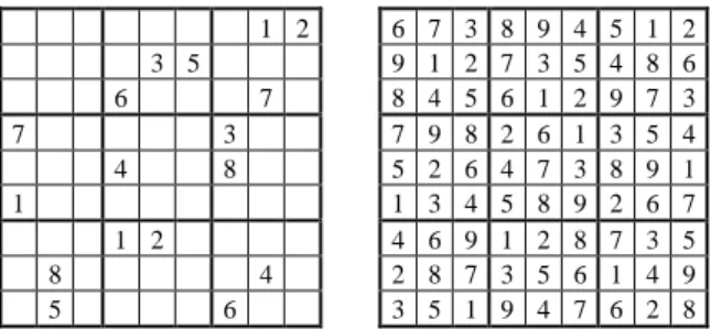
Figure 1.1 shows the standard presentations of a problem grid (also called a
Sudoku puzzle) and of a solution grid (also called a complete Sudoku grid).
Since rows, columns and blocks play similar roles in the defining constraints, they will naturally appear to do so in many other places and a word that makes no
difference between them is widely used in the Sudoku world: a unit is either a row or a column or a block. And one says that two cells share a unit, or that they see each other, if they are different and they are either in the same row or in the same column or in the same block (where “or” is non exclusive). We shall also say that these two cells are linked. It should be noticed that this (symmetric) relation between two different cells, whichever of the three equivalent names it is given, does not depend on the content of these cells but only on their place in the grid; it is therefore a straightforward and quasi physical notion.
1 2 6 7 3 8 9 4 5 1 2 3 5 9 1 2 7 3 5 4 8 6 6 7 8 4 5 6 1 2 9 7 3 7 3 7 9 8 2 6 1 3 5 4 4 8 5 2 6 4 7 3 8 9 1 1 1 3 4 5 8 9 2 6 7 1 2 4 6 9 1 2 8 7 3 5 8 4 2 8 7 3 5 6 1 4 9 5 6 3 5 1 9 4 7 6 2 8
Figure 1.1. A puzzle (Royle17#3) and its solution
As appears from the definition, a Sudoku grid is a special case of a Latin Square. Latin Squares must satisfy the same constraints as Sudoku, except the condition on blocks. Following HLS1, the logical relationship between the two theories will be fully clarified in chapters 3 and 4.
What we need now is to see how the above natural language formulation of the Sudoku problem can be re-written as a CSP. In Chapter 2, the essential question of modelling in general and its practical implications on how to deal with a CSP will be raised and we shall see that the following formalisation is neither the only one nor the best one. But, for the time being, we only want to write the most straightforward one.
For each row r and each column c, introduce a variable Xrc with domain the set
of digits {1, 2, 3, 4, 5, 6, 7, 8, 9}. Then the general Sudoku problem can be expressed as a CSP for these variables, with the following set of (binary) constraints:
Xrc ≠ Xr’c’ for all the pairs {rc, r’c’} such that the cells rc and r’c’ share a unit,
and a particular puzzle will add to these binary constraints the set of unary constraints fixing the values of the Xrc variables corresponding to the givens.
Notice that the natural language phrase “complete the grid” in the original formulation has naturally been understood as “assign one and only one value to each
of the cells” – which has then been translated into “assign a value to each of the Xrc
variables” in the CSP formulation.
1.2. Paradigms of resolution
A CSP states the constraints a solution must satisfy, i.e. it says what is desired. But it does not say anything about how a solution can be obtained; this is the job of resolution methods, the choice of which will depend on the various purposes one may have in addition to merely finding a solution. A particular class of resolution methods, based on resolution rules, will be the main topic of this book.
1.2.1. Various purposes and methods
If one’s only goal is to get a solution by any available means, very efficient general-purpose algorithms have been known for a long time [Kumar 1992, Tsang 1993]; they guarantee that they will either find one solution or all the solutions (according to what is desired) or find a contradiction in the givens; they have lots of more recent variants and refinements. Most of these algorithms involve the combination of two very different techniques: some direct propagation of constraints between variables (in order to progressively reduce their sets of possible values) and some kind of structured search with “backtracking” (depth-first, breadth-first, …, possibly with some forms of look-ahead); they consist of trying (recursively if necessary) a value for a variable and propagating (based on the constraints) the consequences of this tentative choice as restrictions on other variables; eventually, either a solution or a contradiction will be reached; the latter case allows to conclude that this value (or this combination of values simultaneously tried in the recursive case) is impossible and it restricts the possibilities for this (subset of) variables(s).
But, in some cases, such blind search is not possible for practical reasons (e.g. one is not in a simulator but in real life) or not allowed (for a priori theoretical or æsthetic reasons), or one wants to simulate human behaviour, or one wants to “understand” or to be able to “explain” each step of the resolution process (as is generally the case with logic puzzles), or one wants a “constructive” solution (with no “guessing”) or one wants a “pure logic” or a “pattern-based” or a “rule-based” or the “simplest” solution, whatever meaning they associate with the quoted words.
Contrary to the current CSP literature, this book will only deal with the latter cases and more attention will be paid to the resolution path than to the final solution itself. Indeed, it can also be considered as an informal reflection on how notions such as “no guessing”, “a constructive solution”, “a pure logic solution”, “a pattern-based solution”, “an understandable proof of the solution”, “an explanation of the solution” and “the simplest solution” can be defined (but we shall only be able to say more on this topic in the retrospective “final remarks” chapter). It does not mean
that efficiency questions are not relevant to our approach, but they are not our primary goal, they are conditioned by such higher-level requirements. Without these additional requirements, there is no reason to use techniques computationally much harder (probably exponentially much harder) than the general-purpose algorithms.
In such situations, it is convenient to introduce the notion of a candidate, i.e. of a “still possible” value for a variable. As this intuitive notion does not pertain to the CSP itself, it must first be given a clear definition and a logical status. When this is done (in chapter 4), one can define the concepts of a resolution rule (a logical formula in the “condition action” form, which says what to do in some factual, observable situation described by the condition pattern), a resolution theory (a set of such rules), a resolution strategy (a particular way of using the rules in a resolution theory). One can then study the relationship between the original CSP and several of its resolution theories. One can also introduce several properties a resolution theory can have, such as confluence and completeness (contrary to general purpose algorithms, a resolution theory cannot in general solve all the instances of a given CSP; evaluating its scope is thus a new topic in its own; one can also study its statistical resolution power in specific CSP cases).
This “rule-based” or “pattern-based” approach was first introduced in HLS1, in the limited context of Sudoku. It is the purpose of this book to show that it is indeed very general and chapters 14 to 16 will concretely show that it does apply to the very different types of constraints appearing in Futoshiki, Kakuro and map colouring, but let us first illustrate how these ideas work for Sudoku.
1.2.2. Candidates and candidate elimination in Sudoku
The process of solving a Sudoku puzzle “by hand” is generally initialised by defining the “candidates” for each cell. For later formalisation, one must be careful with this notion: if one analyses the natural way of using it, it appears that, at any
stage of the resolution process, a candidate for a cell is a number that has not yet been explicitly proven to be an impossible value for this cell.
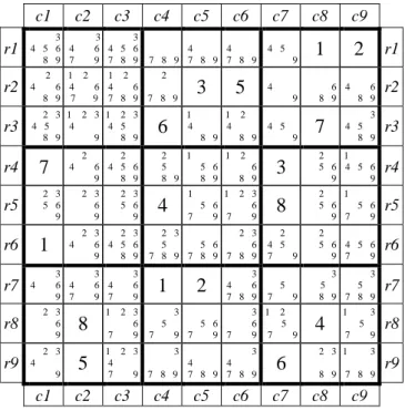
Usually, candidates for a cell are displayed in the grid as smaller and/or clearer digits in this cell (as in Figure 1.2). Similarly, at any stage, a decided value is a number that has been explicitly proven to be the only possible value for this cell; it is written in big fonts, like the givens.
At the start of the game, one possibility is to consider that any cell with no input value admits all the numbers from 1 to 9 as candidates – but more subtle initialisations are possible (e.g. as shown in Figure 1.2) and a slightly different, more symmetric, view of candidates can be introduced (see chapter 2).
Then, according to the formalisation introduced in HLS1, a resolution process that corresponds to the vague requirement of a “pure logic” solution is a sequence of
steps consisting of repeatedly applying “resolution rules” of the general condition-action type: if some pattern – i.e. configuration of cells, possible cell-values, links, decided values, candidates and non-candidates – defined by the condition part of the rule, is effectively present in the grid, then carry out the action(s) specified by the action part of the rule. Notice that any such pattern always has a purely “physical”, invariant part (which may be called its “physical” or “structural” support), defined by conditions on possible cell-values and on links between them, and an additional part, related to the actual presence/absence of decided values and/or candidates in these cells in the current situation. (Again, this will be generalised in chapter 2 with the four “2D” views.)
c1 c2 c3 c4 c5 c6 c7 c8 c9 r1 3 4 5 6 8 9 3 4 6 7 9 3 4 5 6 7 8 9 7 8 9 4 7 8 9 4 7 8 9 4 5 9
1
2
r1 r2 4 6 2 8 9 1 2 4 6 7 9 1 2 4 6 7 8 9 2 7 8 93
5
4 9 6 8 9 4 6 8 9 r2 r3 4 5 2 3 8 9 1 2 3 4 9 1 2 3 4 5 8 96
1 4 8 9 1 2 4 8 9 4 5 97
3 4 5 8 9 r3 r47
2 4 6 9 2 4 5 6 8 9 2 5 8 9 1 5 6 8 9 1 2 6 8 93
2 5 6 9 1 4 5 6 9 r4 r5 2 3 5 6 9 2 3 6 9 2 3 5 6 94
1 5 6 7 9 1 2 3 6 7 98
2 5 6 9 1 5 6 7 9 r5 r61
2 3 4 6 9 2 3 4 5 6 8 9 2 3 5 7 8 9 5 6 7 8 9 2 3 6 7 8 9 2 4 5 7 9 2 5 6 9 4 5 6 7 9 r6 r7 3 4 6 9 3 4 6 7 9 3 4 6 7 91
2
3 4 6 7 8 9 5 7 9 3 5 8 9 3 5 7 8 9 r7 r8 2 3 6 98
1 2 3 6 7 9 3 5 7 9 5 6 7 9 3 6 7 9 1 2 5 7 94
1 3 5 7 9 r8 r9 2 3 4 95
1 2 3 4 7 9 3 7 8 9 4 7 8 9 3 4 7 8 96
2 3 8 9 1 3 7 8 9 r9 c1 c2 c3 c4 c5 c6 c7 c8 c9Figure 1.2. Grid Royle17#3 of Figure 1.1, with the candidates remaining after the elementary constraints for the givens have been propagated
Depending on the type of their action part, such resolution rules can be classified into two categories (assertion type and elimination type):
– either they assert a decided value for a cell (e.g. the Single rule: if it is proven that there is only one possibility left for it); there are very few such assertion rules;
– or they eliminate some candidate(s) (which we call the target(s) of the pattern); as appears from a quick browsing of the available literature, almost all the
classical Sudoku resolution rules are of this type (and, apart from Singles, the few rules that seem to be of the assertion type can be reduced to elimination rules); they express elaborated forms of constraints propagation; their general form is: if such pattern is present, then it is impossible for some number(s) to be in some cell(s) and the target candidates must therefore be deleted; for the general CSP also, all the rules we shall meet in this book, apart from Singles, will be of the elimination type.
The interpretation of the above resolution rules, whatever their type, should be clear: none of them claims that there is a solution with such value asserted or such candidate deleted. Rather, it must be interpreted as saying: “from the current situation it can be asserted that any solution, if there is any, must satisfy the conclusion of this rule”.
From both theoretical and practical points of view, it is also important to notice that, as one proceeds with resolution, candidates form a monotone decreasing set and decided values form a monotone increasing set. Whereas the notion of a candidate is the intuitive one for players, what is classical in logic is increasing monotonicity (what is known / what has been proven can only increase with time); but this is not a real problem, as it could easily be restored by considering non-candidates instead (i.e. what has been erased instead of what is still present).
For some very difficult puzzles, it seems necessary to (recursively) make a hypothesis on the value of a cell, to analyse its consequences and to eliminate it if it leads to a contradiction; techniques of this kind do not fit a priori the above condition-action form; they are proscribed by purists (for the main reason that they often make the game totally uninteresting) and they are assigned the infamous, though undefined, name of Trial-and-Error. As shown in HLS and in the statistics of chapter 6, they are needed in only extremely rare cases if one admits the kinds of chain rules (whips) that will be introduced in chapter 5.
1.2.3. Extension of this model of resolution to the general CSP
It appears that the above ideas can be generalised from Sudoku to any CSP. Candidate elimination corresponds to the now classical idea of domain restriction in CSPs. What has been called a candidate above is related to the notion of a label in the CSP world, a name coming from the domain of scene labelling, which historically led to identifying the general Constraint Satisfaction Problem. However, contrary to labels that can be given a very simple set theoretic definition based on the data defining the CSP, the status of a candidate is not a priori clear from the point of view of mathematical logic, because this notion does not pertain per se to the CSP formulation, nor to its direct logic transcription.
In chapter 4, we shall show that a formal definition of a candidate must rely on intuitionistic logic and we shall introduce more formally our general model of
resolution. Then we shall define the notion of a resolution theory and we shall show that, for each CSP, a Basic Resolution Theory can be defined. Even though this Basic Theory may not be very powerful, it will be the basis for defining more elaborate ones; it is therefore “basic” in the two meanings of the word.
1.3. Parameters and instances of a CSP; minimal instances; classification
Generally, a CSP defines a whole family of problem instances.
Typically, there is an integer parameter that splits this family into subclasses. A good example of such a parameter is the size of the grid in N-Queens, Latin Squares, Sudoku or Futoshiki; in Kakuro, it could be the number of white cells. In the resource allocation problem, it could be some combination of the number of resources and the number of tasks competing for them. In graph colouring and graph matching, it could be the size of the graph (e.g. the number of vertices or some combination of the number of vertices and the number of edges).
1.3.1. Minimal instances
Typically also, once this main parameter has been fixed, there remains a whole family of instances of the CSP. In 9×9 Sudoku, an instance is defined by a set of givens. In N-Queens, although the usual presentation of the problem starts from an empty grid and asks for all the solutions, we shall adopt for our purposes another view of this CSP; it consists of setting a few initial entries and asking for a solution or a “readable” proof that there is none. In “pure” Futoshiki, an instance is defined by a set of inequalities between adjacent cells; in Kakuro by a set of sum constraints in horizontal or vertical sectors. In graph colouring, the possibilities are still more open: there may be lots of graphs of a given size and, once such a graph has been chosen, it may also be required to have predefined colours for some subsets of vertices (although this is a non-standard requirement in graph theory). The same remarks apply to graph matching, where one may want to have predefined correspondences between some vertices (and/or edges) of the two graphs.
In such cases, classifying all the instances of a CSP or doing statistics on the difficulty of solving them meets problems of two kinds. Firstly, lots of instances will have very easy solutions: if givens are progressively added to an instance, until only the values of few variables remain non given, the problem becomes easier and easier to solve. Conversely, if there are so few instances that the problem has several solutions, some of these may be much easier to find than others. These two types of situations make statistics on all the instances somewhat irrelevant. This is the motivation for the following definition (inherited from the Sudoku classics).
Definition: an instance of a CSP is called minimal if it has one and only one solution and any instance obtained from it by eliminating any of its givens has more than one solution. [This is a notion of local minimality.]
For the above-mentioned reasons, all our statistical analyses of a CSP (and only the statistical ones!) will be restricted to the set of its minimal instances.
1.3.2. Rating and the complexity distribution of instances
Classically, the complexity of a CSP is studied with respect to its main size parameter and one relies on a worst case (or more rarely on a mean case) analysis. It often reaches conclusions such as “this CSP is NP-complete” – as is the case for Sudoku(n) or LatinSquare(n), considered as depending on grid size n.
The questions about complexity that we shall tackle in this book are of a very different kind; they will not be based on the main size parameter. Instead, they will be about the statistical complexity distribution of instances of a fixed size CSP.
This supposes that we define a measure of complexity for instances of a CSP. We shall therefore introduce several ratings (starting in chapter 5) that are meaningful for the general CSP. And we shall be able to give detailed results (in chapter 6) for the standard (i.e. 9×9) Sudoku case. In trying to do so, the problem arises of creating unbiased samples of minimal instances and it appears to be very much harder than one may expect. We shall be able to show this in full detail only for the particular Sudoku case, but our approach is sufficiently general to suggest that the same kind of problem is very likely to arise in any CSP; moreover, the final chapters on different logic puzzles will show that they do face the same problem.
Indeed, we shall define measures of complexity associated with various families of resolution rules. For each of them, the complexity of a CSP instance will be defined as the complexity of the hardest rule in this family necessary to solve it, which is also the complexity of the hardest step of the “simplest” resolution path using only rules from this family. Sudoku examples show that a given set of rules can solve puzzles whose full resolution paths vary largely in intuitive complexity (whatever intuitive notion of complexity one adopts for the paths), but the hardest step rating is statistically meaningful; moreover, there is currently no idea about how to formally define the complexity of a full path, i.e. of how to combine in a consistent way the complexities of a sequence of individual steps.
The main advantage of considering ratings of the hardest step type is that, for each family of rules, an associated rank can be defined in a very simple, pure logic way. This naturally leads to an interpretation of our initial “simplest solution” requirement and to the notion of a “simplest-first strategy”.
1.4. The basic and the more complex resolution theories of a CSP
Following the definition of the CSP graph in section 1.1.1, we say that two candidates are linked by a direct contradiction, or simply linked, if there is a constraint making them incompatible (including the obvious “strong” constraints, usually not explicitly stated as such, that different values for a CSP variable are incompatible).
1.4.1. Universal elementary resolution rules and their limitations
Every CSP has a Basic Resolution Theory: BRT(CSP). The simplest elimination rule (obviously valid for any CSP) is the direct translation of the initial problem formulation into operational rules for managing candidates. We call it the “elementary constraints propagation rule” (ECP):
– ECP: if a value is asserted for a CSP variable (as is the case for the givens), then remove any candidate that is linked to this value by a direct contradiction.
The simplest assertion rule (also obviously valid) is called Single (S):
– S: if a CSP variable has only one candidate left, then assert it as the only possible value of this variable.
There is also an obvious Contradiction Detection rule (CD):
– CD: if a CSP variable has no decided value and no candidate left, then conclude that the problem has no solution.
Together, the “elementary rules” ECP, S and CD constitute the Basic Resolution Theory of the CSP, BRT(CSP).
In Sudoku, novice players may think that these three elementary rules express the whole problem and that applying them repeatedly is therefore enough to solve any puzzle. If such were the case, one would probably never have heard of Sudoku, because it would amount to mere paper scratching and it would soon become boring. Anyway, as they get stuck in situations in which they cannot apply any of these rules, they soon discover that, except for the easiest puzzles, this is very far from being sufficient. The puzzle in Figure 1.1 is a very simple illustration of how one gets stuck if one only knows and uses the elementary rules: the resulting situation is shown in Figure 1.2, in which none of these rules can be applied. For this puzzle, modelling considerations related to symmetry (chapter 2) lead to “Hidden Single” rules allowing to solve it, but even this is generally very far from being enough.
1.4.2. Derived constraints and more complex resolution theories
As we shall see later, there are lots of puzzles that require resolution rules of a much higher complexity than those in the Basic Resolution Theory in order to be
solved. And this is why Sudoku has become so popular: all but the easiest puzzles need a particular combination of neuron-titillating techniques and they may even suggest the discovery of as yet unknown ones.
In any CSP, the general reason for the limited resolution power of its Basic Resolution Theory can be explained as follows. Given a set of constraints, there are usually many “derived” or “implied” constraints not immediately obvious from the original ones. Many resolution rules can be considered as a way of expliciting some of the derived unary constraints. As we shall see that very complex resolution rules are needed to solve some instances of a CSP, this will show not only that derived constraints cannot be reduced to the elementary rules of the Basic Resolution Theory (which constitute the most straightforward operationalization of the axioms) but also that they can be unimaginably more complex than the initial constraints.
With all our examples being minimal instances, secondary questions about multiple or inexistent solutions can be discarded. From an epistemological point of view, the gap between the what (the initial constraints) and the how (the resolution rules necessary to solve an instance) is thus exhibited in all its purity, in a concrete way understandable by anyone. [In spite of my formal logic background and of my familiarity with all the well-known mathematical ideas more or less related to it (culminating in deterministic chaos), this gap has always been for me a subject of much wonder. It is undoubtedly one of the main reasons why I kept interested in the Sudoku CSP for much longer than I expected when I first chose it as a topic for practical classes in AI.]
All the families of resolution rules defined in this book can be seen as different ways of exploring this gap – and the consideration of derived binary constraints and/or larger Sudoku grids shows that the gap can be still much larger or deeper than shown by the standard 99 case.
1.4.3. Resolution rules and resolution strategies; the confluence property
One last point can now be clarified: the difference between a resolution theory (a set of resolution rules) and a resolution strategy. Everywhere in this book, a
resolution strategy must be understood in the following extra-logical sense:
– a set of resolution rules, i.e. a resolution theory, plus
– a non-strict precedence ordering of these rules. Non-strict means that two rules can have the same precedence (for instance, in Sudoku, there is no reason to give a rule higher precedence than a rule obtained from it by transposing rows and columns or by any of the generalised symmetries explained in chapter 2).
As a consequence of this definition, several resolution strategies can be based on the same resolution theory with different partial orderings of its rules and they may lead to different resolution paths for a given instance.
Moreover, with every resolution strategy one can associate several deterministic procedures for solving instances of the CSP, as given by the following (sketchy) pseudo-code.
As a preamble (each of the following choices will generate a different procedure): - list all the resolution rules in a way compatible with their precedence ordering (i.e. among the different possibilities of doing so, choose one);
- list all the labels in a predefined order or take them in random order.
Given an instance P, loop until a solution of P is found (or until all the solutions are found or until it is proven that P has no solution):
Do until a rule can effectively be applied: Take the first rule not yet tried in the list
Do until its condition pattern is effectively active:
Try to apply all the possible mappings of the condition pattern of this rule to subsets of labels, according to their order in the list of labels
End do End do
Apply the rule to the selected matching pattern End loop
In this context, a natural question arises: given a resolution theory T, can different resolution procedures built on T lead to an instance being finally solved by some of them and unsolved by others? The answer lies in the confluence property of a resolution theory, to be explained in chapter 5; this fundamental property implies that the order in which the rules of T are applied is irrelevant as long as we are only interested in solving instances (but it can still be relevant when we also consider the efficiency of the procedure): all the resolution paths will lead to the same final state.
This apparently abstract confluence property (first introduced in HLS1) has very practical consequences when it holds in a resolution theory T. It allows any opportunistic strategy, such as applying a rule as soon as a pattern instantiating it is found (e.g. instead of waiting to have found all the potential instantiations of rules with the same precedence before choosing which should be applied first). Most importantly, it also allows to define a “simplest first” strategy that is guaranteed to produce a correct rating of an instance with respect to T after following a single resolution path (with the easy to imagine computational consequences).
1.5. The roles of logic, AI, Sudoku and other examples
As its organisation shows, this book about the general CSP has a large part (about a quarter) dedicated to illustrating the abstract concepts with a detailed case study of Sudoku; to a lesser extent, it also provides examples from various other
logic puzzles. It can be considered as an exercise in either logic or AI or any of these games. Let us clarify the roles we grant each of these topics.
1.5.1. The role of logic
Throughout this book, the main function of logic will be to provide a rigorous framework for the precise definitions of our basic concepts (such as a “candidate”, a “resolution rule” and a “resolution theory”). Apart from the formalisation of the CSP itself, the simplest and most striking example is the formalisation (in section 4.3) of the CSP Basic Resolution Theory informally defined in section 1.4.1 and of all the forthcoming more complex resolution theories. Logic will also be used as a compact notational tool for expressing some resolution rules in a non-ambiguous way. In the Sudoku example, it will also be a very useful tool for expliciting the precise symmetry relationships between different “Subset rules” (in chapter 8).
For better readability, the rules we introduce are always formulated first in plain English and their validity is only established by elementary non-formal means. The non-mathematically oriented reader should thus not be discouraged by the logical formalism. Moreover, all the types of chain rules we shall consider will always be represented in a very intuitive, almost graphical formalism.
As a fundamental and practical application of our strict logical foundations to the Sudoku CSP, its natural symmetry properties can be transposed into three formal meta-theorems allowing one to deduce systematically new rules from given ones (see chapter 2 and sections 3.6 and 4.7). In HLS, this allowed us to introduce chain rules of completely new types (e.g. “hidden chains”). It also allowed the statement of a clear logical relationship between Sudoku and Latin Squares.
Finally, the other role assigned to logic is that of a mediator between the intuitive formulation of the resolution rules and their implementation in an AI program (e.g. our general purpose CSP-Rules solver). This is a methodological point for AI (or software engineering in general): no program development should ever be started before precise definitions of its components are given (though not necessarily in strict logical form) – a commonsense principle that is very often violated, especially by those who consider it as obvious [this is the teacher speaking!]. Notice however that the logical formalism is only one among other preliminaries to implementation (even in the form of rules of an inference engine) and that it does not dispense with the need for some design work (be it only for efficiency matters!).
1.5.2. The role of AI
The role we assign to AI in this book is mainly that of providing a quick testbed for the general ideas developed in the theoretical part. The main rules have been implemented in our general CSP-Rules solver. This was initially designed for
Sudoku only (and accordingly named SudoRules), with input and output functions dedicated to Sudoku, but the hard core (CSP-Rules) can be applied to any CSP and all the examples of chapters 14 to 16 also rely on it. See section 17.4 for more about CSP-Rules and the specific CSPs that have already been interfaced to it.
One important facet of the rules introduced in this book is their resolution power. This can only be tested on specific examples but the resolution of each instance by a human solver needs a significant amount of time and the number of instances that can be tested “by hand” against any resolution method is very limited. On the contrary, implementing our resolution rules in a solver allowed us to test about ten millions of Sudoku puzzles (see chapter 6). This also gave us indications of the relative efficiency of different rules. It is not mere chance that the writing of HLS,
CRT and the present book occurred in parallel with successive versions of
(SudoRules and) CSP-Rules. Abstract definitions of the relative complexities of rules were checked against our puzzle collections for their resolution times and for their memory requirements (in terms of the number of partial chains generated).
This book can also be considered as the basis for a long exercise in AI. Many computer science departments in universities have used Sudoku for various projects. According to our personal experience, it is a most welcome topic for student projects in computer science or AI. This is also true of the other types of puzzles introduced in chapters 14 to 16. Trying to implement some rules, even the “simple” Subset rules of chapter 8 and even in an application-specific way, shows how re-ordering the conditions can drastically change the behaviour of a knowledge-based system: without care, Quads can easily lead to memory overflow problems. (We give detailed formulations for Subset rules in Sudoku, also valid for games based on similar square grids, so that they can be used for such exercises without too long preliminaries.) Trying to implement Sp-whips or Wp-whips is a real challenge.
1.5.3. The role of Sudoku
Because some parts of this book related to the general CSP may seem abstract to the non-mathematician reader (e.g. chapters 3 and 4) or technical (e.g. chapters 9 to 11), a detailed case study was needed to show progressively how the general concepts work in practice. It is also necessary to show how the general theory can easily be adapted, in the most important initial modelling phase, for dealing more efficiently or more naturally with each specific case. Choosing Sudoku for these purposes was for us a natural consequence of the historical development of the techniques described here, both the general approach and all the types of resolution rules. But there are many other reasons why it is an excellent example for the general CSP.
A fast browsing of this book shows that examples from the Sudoku CSP appear in many chapters (generally at the end, in order not to overload the main text with
long resolution paths) and we keep our HLS constraint that all of them should originate in a real minimal puzzle. But it should be clear for the readers of HLS that the purpose here is very different: we have no goal of illustrating with a Sudoku example each of the rules we introduce (for this, there is HLS).
Each example is chosen to satisfy a precise function with respect to the general Constraint Satisfaction Problem, such as providing a counter-example to some conjecture. As a result, most of our Sudoku examples will be exceptional cases, with very long resolution paths – which (without this warning) could give a very bad idea of how difficult the resolution paths look for the vast majority of instances; the statistics in chapter 6 will give a much better idea: most of the time, the chains used and the paths are short.
1.5.3.1. Why Sudoku is a good example
Sudoku is known to be NP-complete [Gary & al. 1979]; more precisely, the CSP family Sudoku(n) on square grids of sizes nn for all n is NP-complete. As we fix n = 9, this should not have any impact on our analyses. But the Sudoku case will exemplify very clearly (in chapter 6) that, for fixed n, the instances of an NP-complete problem often have a broad spectrum of complexity. It will also show that standard analyses, only based on worst case (worst instances) or (more rarely) mean case, can be very far from reflecting the realities of a CSP.
For fixed n = 9, Sudoku is much easier to study than other readily formalised problems such as Chess or Go or any “real world” example. But it keeps enough structure so that it is not obvious.
Sudoku is a particular case of Latin Squares. Latin Squares are more elegant (and somehow more “respectable”) from a mathematical point of view, because they enjoy a complete symmetry of all the types of variables: numbers, rows, columns. In Sudoku, the constraint on blocks introduces some apparently mild complexity that makes it more exciting for players. But this lack of full symmetry also makes it much more interesting from a theoretical point of view. In particular, it allows to introduce the notion of a grouped label (g-label), not present in Latin Squares, and new resolution rules based on it: g-whips and g-braids (see chapter 7). It is noticeable that, with the proper definition of these patterns, they appear (in very different guises) in many other CSPs.
There are millions of Sudoku players all around the world and many forums where the rules defined in HLS have been the topic of much debate. A huge amount of invaluable experience has been cumulated and is available – including generators of random (but biased) puzzles, collections of puzzles with very specific properties (fish patterns, symmetry properties, …) and other collections of extremely hard puzzles. The lack of similar collections and of generators of minimal instances is a strong limitation for the detailed analysis of other CSPs.
1.5.3.2. Origin of our Sudoku examples
Most of our Sudoku examples rely on the following sets of minimal puzzles: – the Sudogen0 collection consists of 1,000,000 puzzles randomly generated by us with the top-down suexg generator (http://magictour.free.fr/suexco.txt), with seed 0 for the random numbers generator; puzzle number n is named Sudogen0#n;
– the cb collection consists of 5,926,343 puzzles we produced with a new kind of generator, the controlled-bias generator (we first introduced it on the late Sudoku Player’s Forum; see also [Berthier 2009] and chapter 6 below); it is still biased, but much less than the previously existing ones and in a precisely known way, so that it allows to compute unbiased statistics; puzzle number n is named cb#n;
– the Magictour collection of 1,465 puzzles considered to be the hardest (at the time of its publishing); puzzle number n is named Magictour-top1465#n;
– the gsf collection of 8,152 puzzles considered to contain the hardest puzzles (at the time of its publishing); puzzle number n is named gsf-top8152 #n;
– the recent eleven collection of 26,370 puzzles not solvable by T&E(S4); puzzle
number n is named eleven#n; we occasionally refer to complementary collections so as to deal with all the known hardest puzzles (see chapter 11).
1.5.4. The role of non Sudoku examples
Although Sudoku is a very good CSP example, it has a few specificities, such as (the major one of) having only “strong” constraints (i.e. all its constraints are defined by CSP variables). With other examples (e.g. N-Queens), we shall show that these specificities have no negative impact on our general theory: the main resolution rules (for whips, g-whips, Subsets, Sp-whips, Wp-whips, braids, …) can
effectively be applied to other CSPs; we shall also illustrate how different these patterns may look in these cases.
We are aware that many more examples should be granted as much consideration as Sudoku. We hope that the final chapters partially palliate this shortcoming by considering CSPs based on constraints of very different kinds (transitive in Futoshiki, non-binary arithmetic in Kakuro, topological and geometric in Map colouring, Numbrix® and Hidato®). We also hope that this book will
motivate more research for applications to other CSPs.
1.5.5. Uniform presentation of all the examples
If we displayed the full resolution path of an instance, it would generally take several pages, most of which would describe obvious or uninteresting steps. We shall skip most of these steps, by adopting the following conventions (the same as in
– elementary constraint propagation rules (ECP) will never be displayed; – as the final rules that apply to any instance are always ECP and Singles (at least when these rules are given higher priority than more complex ones – which is a natural choice), they will be omitted from the end of the path.
All our examples respect the following uniform format. After an introductory text explaining the purpose of the example, the resolution theory T applied to it and/or comments on some particular point, a row of two (sometimes three) grids is displayed: the original puzzle (sometimes an intermediate state) and its solution. Then comes the resolution path, a proof of the solution within theory T, where
“proof” is meant in the strict sense of intuitionistic/constructive logic.
Each line in the resolution path consists of the name of the rule applied, followed by: the description of how the rule is “instantiated” (i.e. how the condition part is satisfied), the “==>” sign, the conclusion allowed by the “action” part. The conclusion is always either that a candidate can be eliminated (symbolically written as r4c8 ≠ 6 in Sudoku) or that a value must be asserted (symbolically written as r4c8 = 5). When the same rule instantiation justifies several conclusions, they are written on the same line, separated by commas: e.g. r4c8 ≠ 8, r5c8 ≠ 8. Occasionally, the detailed situation at some point in the resolution path (the “resolution state”) is displayed so that the presence of the pattern under discussion can be directly checked, but, due to place constraints, this cannot be systematic.
All the resolution paths given in this second edition were obtained with version 1.2 of our general pattern-based CSP solver: CSP-Rules1 (with occasional hand editing for a shorter and/or cleaner appearance), using the CLIPS inference engine (release 6.30), on a MacPro® 2006 running at 2.66 GHz. It was easily supplemented
with inpout/output functions specific to Sudoku (making it correspond to version 15d.1.12 of our SudoRules solver), Futoshiki, Kakuro, Map colouring, Numbrix® and Hidato®.
1.6. Notations
Throughout this book, we consider an arbitrary, but fixed, finite Constraint Satisfaction Problem. We call it CSP, generically. BRT(CSP) or simply BRT (when there is no ambiguity) refers to its Basic Resolution Theory, RT to any of its resolution theories, Wn [respectively Bn, gWn, gBn, SpWn, SpBn, BpBn, …] to its nth
whip [respectively braid, g-whip, g-braid, Sp-whip, Sp-braid, Bp-braid, …] resolution
theory. The same letters, with no n subscript, are used for the associated ratings.
1