HAL Id: hal-01710759
https://hal.archives-ouvertes.fr/hal-01710759
Submitted on 16 Feb 2018
HAL is a multi-disciplinary open access
archive for the deposit and dissemination of
sci-entific research documents, whether they are
pub-lished or not. The documents may come from
L’archive ouverte pluridisciplinaire HAL, est
destinée au dépôt et à la diffusion de documents
scientifiques de niveau recherche, publiés ou non,
émanant des établissements d’enseignement et de
Minimal controllability time for finite-dimensional
control systems under state constraints
Jérôme Lohéac, Emmanuel Trélat, Enrique Zuazua
To cite this version:
Jérôme Lohéac, Emmanuel Trélat, Enrique Zuazua.
Minimal controllability time for
finite-dimensional control systems under state constraints. Automatica, Elsevier, 2018, 96, pp.380-392.
�10.1016/j.automatica.2018.07.010�. �hal-01710759�
Minimal controllability time for finite-dimensional control
systems under state constraints
J´
erˆ
ome Loh´
eac
*Emmanuel Tr´
elat
Enrique Zuazua
February 16, 2018
Abstract
We consider the controllability problem for finite-dimensional linear autonomous control systems, under state constraints but without imposing any control constraint. It is well known that, under the classical Kalman condition, in the absence of constraints on the state and the control, one can drive the system from any initial state to any final one in an arbitrarily small time. Furthermore, it is also well known that there is a positive minimal time in the presence of compact control constraints. We prove that, surprisingly, a positive minimal time may be required as well under state constraints, even if one does not impose any restriction on the control. This may even occur when the state constraints are unilateral, like the nonnegativity of some components of the state, for instance. Using the Brunovsky normal forms of controllable systems, we analyze this phenomenon in detail, that we illustrate by several examples. We discuss some extensions to nonlinear control systems and formulate some challenging open problems.
1
Introduction
Let n∈ IN∗
and m∈ IN∗
be integers, with m< n. Let A be a n × n matrix and B be a n × m matrix, with real coefficients, satisfying the Kalman condition
rank(B, AB, . . . , An−1B) = n. (1.1) Throughout the paper, we consider the linear autonomous control system
˙
y(t) = Ay(t) + Bu(t) (1.2a) with some initial condition
y(0) = y0 (1.2b) where y(t) ∈ IRn is the state and u(t) ∈ IRm is the control. In order to avoid confusion, we will sometimes write y(t; u) the solution of (1.2). It is well known that, given any two points y0 and
*Universit´e de Lorraine, CRAN, UMR 7039, Centre de Recherche en Automatique de Nancy, 2 avenue de la forˆet de Haye, 54516 Vandœuvre-l`es-Nancy Cedex, France;
CNRS, CRAN, UMR 7039, France ([email protected]).
Sorbonne Universit´e, Universit´e Paris-Diderot SPC, CNRS, Inria, Laboratoire Jacques-Louis Lions, ´equipe CAGE, F-75005, Paris, France ([email protected]).
DeustoTech, Fundaci´on Deusto, Avda Universidades, 24, 48007, Bilbao, Basque Country, Spain; Departamento de Matem´aticas, Universidad Aut´onoma de Madrid, 28049 Madrid, Spain;
Facultad Ingenier´ıa, Universidad de Deusto, Avda. Universidades, 24, 48007 Bilbao, Basque Country, Spain; Sorbonne Universit´e, Universit´e Paris-Diderot SPC, CNRS, Laboratoire Jacques-Louis Lions, F-75005, Paris, France ([email protected]).
y1 of IRn and given any time T > 0, there exists a control u ∈ L∞((0, T ), IRm) such that the corresponding trajectory, solution of (1.2), satisfies y(T ) = y1. In other words, one can pass from any initial condition to any final one in arbitrarily small time. Of course, this is at the price of using controls that have a L∞-norm that is larger as the transfer time T is smaller [25]. Therefore, under the Kalman condition (1.1), if there is no state and control constraint in the control problem, then the minimal controllability time, defined as the infimum of times required to pass from y0 to y1, is equal to 0.
Now, we consider a connected subset C⊂ IRn with nonempty interior, standing for state con-straints that we want to impose to the controllability problem, and we address the following question:
Given any two points y0 and y1 in C, is it possible to steer the control system (1.2) from y0 to y1 in arbitrarily small time T , while guaranteeing that y(t) ∈ C for every t∈ [0, T ], or is there a positive minimal time required?
We stress that we impose no control constraint, i.e., u(t) ∈ IRm, but we impose a state constraint. It is surprising that this apparently simple question has not been investigated before. It is the main objective of this paper to explore it.
Before going further, it is useful to note that controllability under control constraints but without state constraints is well understood (see [4]) and can be studied by usual optimal control methods (see [20, 28]). Recall that, when there is a control constraint u(t) ∈ Ω with Ω a compact subset of IRm then the set AccΩ(y0, T) of accessible points from y0 in time T > 0 with controls u∈ L∞((0, T ), Ω) is compact and convex and evolves continuously with respect to T : hence in this case the minimal time required to pass from y0to y1≠ y0is always positive.
Here, in contrast, we want to investigate the question of knowing whether the minimal time may be positive when imposing state constraints but no control constraint. Of course, in order to address this question we may first wonder whether the target point y1 is reachable or not from the initial point y0. This is the question of controllability under state constraints, which is not the objective of the present paper but on which we shortly comment hereafter.
Controllability under state constraints. When C is a proper subset of IRn, the question of controllability under the state constraint y(⋅) ∈ C is complicated. Even under the Kalman condition, very simple state constraints can immediately make fail the controllability property. For instance, take the control system in IR2
˙
y1(t) = y2(t), y2(t) = u(t),˙
and the state constraint y2(t) ⩾ 0 on the second component of the state. For any trajectory, the first component y1(t) must be nondecreasing, and then obviously one cannot pass from any point to any other.
Controllability under state constraints has not been much investigated in the literature, certainly due to the difficulty of the question, even for linear control systems. Early conditions were given in [17], with the idea of deriving conic directions of expansion of the reachable set. A more achieved version appears in [18], where the author states a necessary and sufficient condition for small-time controllability of linear control systems under conic state constraints. The verification of such algebraic conditions (given in terms of convex hull) remain however quite technical. In [14], controllability is established under appropriate invertibility conditions of the transfer matrix and adequate Hautus test conditions. We also mention the recent paper [19] for sufficient controllability conditions for nonlinear control systems.
In this paper, our objective is, when we already know that y1 can be reached from y0 under state constraints, to investigate whether the minimal time may be positive or not, while keeping the connecting trajectory in the set C.
It is anyway interesting to note that there is a specific situation under which controllability under state constraints can easily be proved, within a transfer time that may however be quite large. This is when y0 and y1 are steady-states (a point ¯y ∈ C is a steady-state if there exists ¯
u∈ IRm such that A¯y+ B¯u = 0). This situation is studied in Section 4.1. More precisely, we prove in this section that, under a slight condition on the set C (which is satisfied if C is convex), it is possible to steer the control system (1.2) from any steady-state y0∈ ˚C to any steady-state y1∈ ˚C in time sufficiently large, while ensuring that the corresponding trajectory remains in the interior ˚
C of the set C. The proof is done by an iterative use of a local controllability result along a path of steady-states (whence the possibly large transfer time). The question is then to know whether one could find a control for which this transfer time would be arbitrarily small.
Minimal controllability time. We investigate the minimal time problem for the system (1.2) under state constraints y(⋅) ∈ C, without control constraint. Given y0, y1∈ C, we define TC(y0, y1) as the infimum of times required to pass from y0 to y1 under the state constraint C (with an unconstrained L∞control), with the agreement that TC(y0, y1) = +∞ if y1is not reachable from y0. More precisely, if y1is reachable from y0, with L∞controls, we define
TC(y0
, y1) = inf {T > 0 ∣ ∃u ∈ L∞((0, T ), IRm) s.t. the solution y(t) of (1.2) satisfies
y(T ) = y1 and ∀t ∈ [0, T ], y(t) ∈ C}. It is obvious that if r = rank B = n then TC(y0, y1) = 0 for any y0 and y1 belonging to a same connected component of C. More precisely, given any time T > 0 and any C1-path, ¯y such that ¯y(0) = y0, ¯y(T ) = y1 and ¯y(t) ∈ C for every t ∈ [0, T ], then any control ¯u, satisfying B ¯u(t) = ˙¯y(t)−A¯y(t), steers the solution of (1.2) to y1in time T . Hence, in what follows we assume that r< n.
As a first example (more details are given in Example 5.1 further), consider the linear control system
˙
y1(t) = y1(t) + u(t), y2(t) = 2y2(t) + u(t),˙
under the nonnegativity state constraints y1(⋅) ⩾ 0, y2(⋅) ⩾ 0, and take the terminal conditions y0 = (1, 1/2)⊺ and y1 = (2, 1)⊺. Both points are steady-states, C = [0, +∞)2 is convex and the Kalman rank condition is satisfied. Hence, it is possible to steer the system from y0 to y1 with a trajectory satisfying the state constraints (see Section 4.1). But we claim that this cannot be done in arbitrarily small time. Here, the value of the minimal time under the state constraint y(⋅) ∈ C is TC(y0, y1) = ln(2). In contrast, steering the control system from y1 to y0 in C can be done in arbitrarily small time, i.e., we have TC(y1, y0) = 0.
The main result of the paper is the following. Theorem 1.1. Let C be a subset of IRn and let y0∈ C.
(i) Let y1∈ ˚C∖ {y0}. Assume that y0∈ ˚C and there exists a steady state ¯y∈ ˚C. If ¯y and y1 are in a same connected component of({y0} + Ran B) ∩ ˚C, then TC(y0, y1) = 0.
(ii) Assume that C is bounded and let y1∈ C ∖ {y0}. If y1− y0∉ Ran(B) then TC(y0, y1) > 0. (iii) Assume that
C= {y ∈ IRn ∣ ⟨`, y⟩ = `1y1+ ⋯ + `nyn⩾ β} (1.3) (unilateral and affine state constraint) for some β∈ IR and for some generic1 `∈ IRn∖ {0}.
If r = rank B > 1 then under a generic2condition on the pair(A, B) we have TC(y0, y1) = 0 for any y0, y1∈ ˚C.
If r = 1 or if the above generic condition is not satisfied then there exists an open subset C1⊂ C such that TC(y0, y1) > 0 for every y1∈ C1.
Note that, in the statement (i) of the theorem, when y1− y0 ∈ Ran(B), even if the segment [y0, y1] is contained in ˚C, it may happen that TC(y0, y1) > 0 (see the example given in Section 2.6). The statement (ii) says that imposing a bounded state constraint creates a positive minimal time. More strikingly, the statement (iii) shows that an unilateral (and thus, unbounded) state constraint may as well create a positive minimal time, depending on the position of the terminal points. It is interesting to note that, for such an unilateral state constraint, the positive minimal time property occurs generically only for m= 1 (only one scalar control).
However, this Theorem does not establish the existence of a control in the minimal time and the existence of such a control is open. As we will indicate further in Section 2.7, we can expect that a minimal time control exists in a wider class of controls.
An additional question discussed in this paper is: does the minimal time defined with L∞controls coincide with the minimal time defined with a wider class of controls?
The proof of Theorem 1.1, done in Section 2, consists of a series of very simple arguments consisting of reductions using Brunovsky normal forms. For the unilateral state constraint (1.3), it reduces our study to the investigation of a linear control system under a nonnegativity constraint on one of the controls.
The statement (iii) of Theorem 1.1 can be easily extended to the case where we consider k unilateral state constraints, i.e. with C= {y ∈ IRn ∣ L⊺y⩾ β}, with L a n × k matrix and β ∈ IRk. With similar arguments as the one used for the proof of Theorem 1.1, it is possible to show that
If r = rank B > k, then under a generic condition on A, B and L, we have TC(y0, y1) = 0 for any y0, y1∈ C;
If m ⩽ k, then under a generic condition on A, B and L, there exists an open subset C1⊂ C such that TC(y0, y1) > 0 for every y1∈ C1.
Since the proof of this result is a slight modification of the one of Theorem 1.1, and since this proof requires more technical notations, we did not provide here the proof of this result.
Heuristic arguments and comments. An intuition suggesting that the minimal controllability time may be positive is the following. We explain it by assuming that m= 1, i.e., in the case where the control is scalar; in this case the matrix B is a (nonzero) vector in IRn. Since there is no constraint on the control u, one can use large control inputs, which behave like impulsive controls, (e.g., approximations of Dirac masses). In particular, in this sense, one can move almost instantaneously in the directions given by B, that is, parallel to B, by taking u(t) = M (or −M) over a small time interval, with M> 0 very large. For instance, if the system is at state y at the instant of time t, and if one takes an impulsive control input in the direction B, then one can move in arbitrarily small time to any point of the affine line y+IRB. But then, according to the shape of the set C, the state constraint y(⋅) ∈ C may prevent the trajectory from moving too far along this line and may then constrain the motion, forbidding one to use such impulses that are not actually admissible because of the state constraint.
Now, in order to move along other directions, for instance, parallel to AB, one usually takes a succession of arcs: u = +M, then u = −M, over small time intervals, with M > 0 very large.
2The word generic means here that the pair (A, B) belongs to an open and dense subset of the set of matrices (A, B) with A (resp. B) a n × n (resp. n × m) matrix.
This corresponds to moving along Lie brackets (see [7, Section 3.2 and comments page 133]). Geometrically, this means that, in order to make one step in some direction AB, one needs to go first very far in the direction B and then maybe in the direction−B. This can indeed be done if there is no state constraint. But, as above, the state constraint y(t) ∈ C may forbid to be able to achieve such a motion.
When m> 1, these comments are still valid by replacing the vector B above by any nontrivial vector of Ran(B), the range of the n × m matrix B.
Of course, the above arguments do not make a rigorous proof but anyway suggest the possible occurrence of a positive minimal time due to state constraints, even if the state constraint is unilateral.
Since the controls are unconstrained, trajectories going from y0 to y1 can move arbitrarily quickly as long as they are in the interior of the authorized region C (in other words, outside of C jumps are allowed) but there is a “loss of time” along the boundary ∂C. This is easily understood by writing (at least locally) C= {y ∈ IRn ∣ c(y) ⩽ 0} for some function c ∶ IRn → IR of class C1: indeed, along a boundary arc, one has c(y(t)) = 0 and by derivating in time we get
⟨∇c(y(t)), Ay(t)⟩ + ⟨B∗∇c(y(t)), u(t)⟩ = 0.
Thus, along ∂C, the motion should be done in minimal time under this new mixed state and control constraint. For instance, if m= 1 and if ⟨∇c(y), B⟩ ≠ 0 for every y ∈ ∂C (meaning that the state constraint is of order one [3]), then the boundary control must be
u(t) = u(y(t)) = −⟨∇c(y(t)), Ay(t)⟩ ⟨∇c(y(t)), B⟩
and generates a boundary arc that travels at finite speed (following the flow of ˙y(t) = Ay(t) + Bu(y(t))), thus creating a positive minimal time. This situation is similar for higher-order state constraints where one needs to differentiate several times before making the control appear explic-itly (see [3]) and in any case, since the value of the control cannot be arbitrarily large, this causes a “loss of time” along the boundary arc.
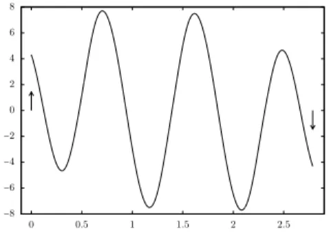
For 2D systems, the situation is quite well understood and this will be developed in Section 5. In the 2D case it is also easy to illustrate the above informal arguments. This is done on Figure 1 (see also Remark 5.1, and Figure 3, for more details on this computation). For this figure, we have considered the system ˙y1= y2, ˙y2= u, under the state constraint y2(t) ⩽ ϕ(y1(t)), for some positive C1 function ϕ.
1. Since the initial point,(y10, 0)⊺ is in the interior of the set of state constraints, one can move with arbitrarily large velocity in the direction generated by B= (0, 1)⊺. At the formal limit, this corresponds to an impulse control (Dirac mass) at the initial time. This impulse is such that the trajectory instantaneously reaches the boundary of the state constraint, at the boundary point(y10, ϕ(y01))⊺ and the corresponding Dirac impulse control is ϕ(y10)δ0. 2. The control is then tuned to follow the state constraint until the point (y1
1, ϕ(y11)). This causes a ”loss of time”.
3. From the point(y1
1, ϕ(y11))
⊺, it is finally possible to instantaneously reach the target(y1 1, 0)
⊺ with a Dirac impulse control.
These rather informal considerations explain why a positive minimal time may be expected to occur, due to state constraints (even unilateral) and although there is no control constraint.
0 0.5 1 1.5 2 2.5 y0 1 y11 −1.5 −0.5 0 0.5 1.5 y2 y1 Forbidden zone Limit state trajectory
(a) State trajectories in the limit case
−8 −6 −4 −2 0 2 4 6 8 0 0.5 1 1.5 2 2.5
(b) Control in the limit case (arrows stands for Dirac masses).
Figure 1: Limit trajectories for the 2D Brunovsky system ˙y1 = y2, ˙y2 = u, with initial point y0= (0, −1)⊺ and target y1= (0, 1)⊺.
Article organization. The article is structured as follows: Theorem 1.1 is proved in Section 2.
In Section 3 we provide several extensions of Theorem 1.1, considering nonlinear control-affine systems under unilateral state constraints.
Section 4 is devoted to establishing several further facts: controllability in large time among the set of steady-states (Section 4.1); there is no classical control exactly at the minimal time (Section 4.2); the minimal time with unbounded controls is the limit of the minimal time under the additional control constraint∣u(⋅)∣ ⩽ M as M → +∞ (Section 4.3).
In Section 5 we compute explicitly the minimal transfer time in 2D (Proposition 5.1) and we give several examples.
Section 6 is a conclusion listing some open problems.
2
Proof of Theorem 1.1
In this section, we give the proof of Theorem 1.1. The statement (i) is proved in Section 2.1. For the other statements, we proceed in three steps (Sections 2.2 to 2.4). These steps are summarized in a concluding section (Section 2.5). We illustrative this result with an example in Section 2.6 and we give some additional comments on this proof in Section 2.7.
2.1
Proof of statement (i)
It suffices to prove that y0(respectively ¯y) can be steered in arbitrarily small time to ¯y (respectively y1). By reversing the time (t↦ T − t), proving that ¯y can be steered to y1in arbitrarily small time is equivalent to proving that y1can be steered to ¯y in arbitrarily small time. Consequently, for the proof, we assume that y1 is a steady state, y1≠ y0, and that there exists ¯v∈ C1([0, 1], IRm) such that ¯v(0) = 0, y0+ B¯v(1) = y1 and for every s∈ [0, 1], y0+ B¯v(s) ∈ ˚C.
For some M > 0, we take as control uM(t) = M ˙¯v(Mt), for t ∈ [0, 1/M]. Then as M → ∞, for every s∈ [0, 1], yM(s/M) → y0+ B¯v(s). This ensures that for M > 0 large enough, yM(t) ∈ ˚C for
every t∈ [0, 1/M] and yM(1/M) is in a neighborhood of y1. Using small time local controllability around y1, we obtain that yM(1/M) can be steered to y1 in some time τ= τ(M), while the state constraint is preserved. In addition, since yM(1/M) converges to y1as M→ ∞, we also have that τ(M) converges to 0 as M → ∞. This ends the proof of statement (i) of Theorem 1.1.
2.2
First step: feedback equivalence and dynamic Brunovsky normal
form
First of all, since no constraint is imposed on the control, one can perform a feedback equivalence in order to obtain a (sometimes called “dynamic”) Brunovsky normal form for (1.2).
We recall that the pair(A, B) is feedback equivalent to ( ˜A, ˜B) if there exist an invertible matrix P of size n× n, an invertible matrix V of size m × m and a matrix F of size m × n such that P−1(A + BF )P = ˜A and P−1BV = ˜B. Feedback equivalence corresponds to make the changes of variables y= P ˜y and u = F y + V ˜u, where ˜y is the new state and ˜u is the new control. The new control system is
˙˜
y(t) = ˜A˜y(t) + ˜B ˜u(t). (2.1) Note that( ˜A, ˜B) satisfies the Kalman condition as well, that the new state ˜y(t) is submitted to the state constraint ˜y(⋅) ∈ P−1C, and that the new control ˜u(⋅) ∈ IRm is still unconstrained. In addition, if ¯y is a steady state for the system (1.2), then P−1y is a steady state as well for the¯ system (2.1). For the unilateral and affine state constraint (1.3), the constraint ˜y(⋅) ∈ P−1C gives ⟨˜`, ˜y(⋅)⟩ ⩾ β with ˜`= P⊺`.
The multi-input Brunovsky normal form theorem (see, e.g., [27]) asserts that, if(A, B) satisfies the Kalman condition and if rank(B) = r ⩽ m then the pair (A, B) is feedback equivalent to the pair of matrices given by
A= ⎛ ⎜⎜ ⎜ ⎝ Ak1 0 ⋯ 0 0 ⋱ ⋱ ⋮ ⋮ ⋱ ⋱ 0 0 ⋯ 0 Akr ⎞ ⎟⎟ ⎟ ⎠ and B= ⎛ ⎜⎜ ⎜ ⎝ bk1 0 ⋯ 0 0 ⋯ 0 0 ⋱ ⋱ ⋮ ⋮ ⋮ ⋮ ⋱ ⋱ 0 ⋮ ⋮ 0 ⋯ 0 bkr 0 ⋯ 0 ⎞ ⎟⎟ ⎟ ⎠ (2.2)
where the indices ki∈ {1, . . . , n} (i ∈ {1, . . . , r}) satisfy k1+ ⋅ ⋅ ⋅ + kr= n and where we have defined the matrices Ak= ⎛ ⎜⎜ ⎜⎜ ⎜ ⎝ 0 1 0 ⋯ 0 ⋮ ⋱ ⋱ ⋱ ⋮ ⋮ ⋱ ⋱ 0 ⋮ ⋱ 1 0 ⋯ ⋯ ⋯ 0 ⎞ ⎟⎟ ⎟⎟ ⎟ ⎠ and bk= ⎛ ⎜⎜ ⎜ ⎝ 0 ⋮ 0 1 ⎞ ⎟⎟ ⎟ ⎠ (2.3)
of respective sizes k× k and k × 1 for any k ∈ IN∗
. Here, we have dropped the tildes in order to keep a better readability. Writing y= (y1, . . . , yr) ∈ IRk1× ⋅ ⋅ ⋅ × IRkr and u= (u1, . . . , um)⊺, the control system (2.1) is
˙
yi= Akiyi+ bkiui, i= 1, . . . , r, (2.4)
with unconstrained controls u1, . . . , ur.
This transformation has no impact on the minimal controllability time and the minimal time TC(y0, y1) for the system (1.2) with state constraint C is equal to the minimal time TC(P−1y0, P−1y1) for the system (2.1) with state constraint P−1C. Let us also give the generic assumption on ` men-tioned in the statement (iii) of Theorem 1.1:
In other words, we make the generic assumption that P P⊺` is not a steady state for the system (1.2) in the initial coordinates.
Based on these considerations, we assume, without loss of generality, that the system (1.2) is already in Brunovsky form (i.e. the matrices A and B are given by (2.2) and ` is not a steady state).
2.3
Second step: reduction by Goh transformation
Let us first explain the idea when there is only one block in (2.4), i.e., when r= 1. We have then the control system
˙
y1,1= y1,2, ˙y1,2= y1,3, . . . , ˙y1,k1−1= y1,k1, ˙y1,k1= u1.
Since the control u1 is unconstrained, the Goh transformation consists of reducing the above system of one dimension by considering y1,k1 itself as a new control. In other words, this is as if we would take u1as Dirac masses and then allow y1,k1 to have discontinuities. This well known idea, consisting in replacing the control by its primitive and then in considering part of the state as a new control, is referred to as the Goh transformation. Introduced in [12], this transformation has often been used to derive second-order necessary and/or sufficient conditions for optimality and is related to the notion of cheap control (see [2]).
Let us now explain how this transformation has an impact on the state constraint y(⋅) ∈ C. Assume that this state constraint only acts on the j1+ 1 first coordinates y1,1, . . . , y1,j1+1. Then one can reiterate the Goh transformation k1− j1 times, until, indeed, y1,j1+1 itself has become a control.
Then, for the reduced control system in dimension j1, where the state is z1= (y1,1, . . . , y1,j1) and
the control is v1= y1,j1+1, the new constraint is(z1(⋅), v1(⋅)) ∈ C, which is now a mixed state and
control constraint.
For instance, for the unilateral and affine state constraint (1.3), written here as `1,1y1,1(⋅) + ⋯ + `1,k1y1,k1(⋅) ⩾ β where `i = (`i,1, . . . , `i,ki) ∈ IRki, the above assumption means that `1,j
1+2= ⋯ =
`1,k1= 0. Hence, at the end of the series of Goh transformations, we have obtained the mixed state and control constraint `1,1y1,1(⋅) + ⋯ + `1,j1y1,j1(⋅) + `1,j1+1v1(⋅) ⩾ β.
In general, doing so for each block in (2.4), we obtain that the minimal controllability time TC(y0, y1) is not lower than the minimal time for steering the control system (living in lower dimension)
˙
zi(t) = Ajizi(t) + bjivi(t) i = 1, . . . , s
from the initial point(z10, . . . , zs0) to the final point (z11, . . . , zs1) with unconstrained controls, under the mixed state and control constraint
(z1(⋅), v1(⋅), . . . , zs(⋅), vs(⋅)) ∈ C.
The novelty here is that, at the previous step we had a pure state constraint, and now due to the Goh transformation we have obtained a mixed state and control constraint indeed acting in a nontrivial way, in particular, on the controls vi.
At this stage, the second point of the statement (ii) of the theorem easily follows, i.e., imposing a bounded state constraint creates a positive minimal time. This is so since the new controls v1, . . . , vsare bounded. This completes the proof of statement (ii) of Theorem 1.1.
Let us now establish the statement (iii), by considering the unilateral and affine state con-straint (1.3). We denote `= (`1, . . . , `r) ∈ IRk1×⋅ ⋅ ⋅×IRkr, with indices kiorganized so that ki= 1 for
i> s and ki > 1 for i ⩽ s. Then, the assumption that ` is not a steady-state ensures the existence of i0∈ {1, . . . , s} and j0∈ {2, . . . , ki0} such that the j0th coefficient of `i0 is nonzero. Without loss
γ= `1,j0 the value of this coefficient. By performing k1− j0+ 1 Goh transformations on the control u1, we obtain that the minimal control time TC(y0, y1) is not lower than the minimal time for steering the control system
˙
z1(t) = Aj0−1z1(t) + bj0−1v1(t)
˙
yi(t) = Akiyi(t) + bkiui(t) i = 2, . . . , r
(2.5)
from the initial point(z10, y02, . . . , yr0) to the final point (z11, y21, . . . , y1r) with controls v1, u2, . . . , ur∈ L∞(0, T ) under the mixed state and control constraint
⟨̂`1, z1(⋅)⟩ + γv1(⋅) + ⟨`2, y2(⋅)⟩ + ⋅ ⋅ ⋅ + ⟨`r, yr(⋅)⟩ ⩾ β
where z1 (resp., ̂`1) is the vector consisting of the first j0− 1 components of y1 (resp., `1). Recall that the matrices Ak and bk are defined by (2.3) for every k∈ IN∗
.
At this step, we have therefore reduced our initial problem to the minimal time problem for a linear control system with r scalar controls among which r− 1 controls are unconstrained. More generally, we have shown that the minimal control time TC(y0, y1) is not lower than the minimal time for
˙
y(t) = Ay(t) + Bu(t)
⟨α, y(⋅)⟩ + γu1(⋅) ⩾ β, (2.6) where the pair(A, B) satisfies the Kalman condition and γ ∈ IR ∖ {0}. Here, A (resp. B and α) is a N× N matrix (resp. N × r matrix and vector of IRN) with N= n − k1+ j0− 1. In order to avoid new notations, we keep denoting n instead of N and m instead of r.
2.4
Third step: change of control
Considering (2.6), we replace the control u with the new control ¯u given by ¯u1= ⟨α, y⟩ + γu1− β and ¯ui= γui for i> 1 and we thus obtain the new control system
˙ y(t) =1γ(γA − b1α⊺)y(t) +1 γB ¯u(t) + β γb1 ¯ u1(⋅) ⩾ 0
where b1 is the first column of B and the control ¯u∈ L∞((0, T ), IRm) is constrained to have a nonnegative first component. Let us also notice that the pair(γA − b1α⊺, B) satisfies the Kalman condition.
At this step, we have reduced the constraint on the control to an unilateral (nonnegativity) constraint on the first component of the control.
Hence, without loss of generality, we consider the minimal time problem for the linear control system
˙
y(t) = Ay(t) + Bu(t) + r
u1(⋅) ⩾ 0 (2.7)
with A (resp. B and r) a n× n matrix (resp. n × m matrix and vector of IRn) and the pair(A, B) satisfies the Kalman condition, with m scalar controls among which the m− 1 last controls are unconstrained and the first control is subject to an unilateral (nonnegativity) constraint. In order to establish the statement (iii) of Theorem 1.1, we only need to prove that for every initial state y0∈ IRn, there exists a target state y1∈ IRn that cannot be reached in arbitrarily small time by a solution of (2.7) such that y(0) = y0.
More precisely, given any time T> 0 and any solution y of (2.7) such that y(0) = y0, we have y(T ) ∈ (eT Ay0+ ∫ T 0 e(T −t)Ar dt) + Acc+(T ) where Acc+ (T ) = { ∫0Te(T −t)ABu(t) dt ∣ u ∈ L∞((0, T ), IRm), u1(⋅) ⩾ 0}.
is the set of accessible points with controls u having a nonnegative first component. It is easy to see that Acc+(T ) is a convex cone with vertex at 0 and that Acc+(T1) ⊂ Acc+(T2) if T1< T2. It would be compact and evolve continuously with respect to T if there were to be a compact constraint on the controls (see [20, 28]); but here, we only have an unilateral constraint on u.
In the next lemma, we denote by b1the first column of B and by ˆB the n× (m − 1) matrix formed by the remaining columns of B (when m= 1, we have B = b1).
Lemma 2.1. If m> 1 and if the pair (A, ˆB) satisfies the Kalman condition then Acc+(T ) = IRn for every T> 0.
Otherwise, if m= 1 or if the pair (A, ˆB) does not satisfy the Kalman condition, then Acc+(T ) is a convex cone with vertex at 0, which is isomorphic to the positive quadrant of IRn for T > 0 small enough.
We stress that this result is only valid in small time. Indeed, for N= 2 consider the matrices A = (−1 0)0 1 , b= (0
1).
We have m= 1, and we claim that Acc+(T ) = IR2 for every T > 2π. Indeed, consider the corre-sponding control system and let it start at (0, 0) at time 0. On a first interval [0, ε) with ε > 0 small, take u(t) = 1, so we steer the system to some point that is close but distinct from the origin. Then, take u= 0 and wait: the corresponding trajectory runs at speed 1 along a circle centered at the origin. This is the way that in time greater than 2π one can indeed reach any point of the plane.
This simple example shows that, although Acc+(T ) is a proper subset of IRn for T > 0 small, it may evolve discontinuously in time and become equal to the whole IRnfor T > T0, for some T0> 0. Proof. The first claim is clear. Let us prove the second claim. Consider first the case m= 1. We consider the system ˙y = Ay + b1u1. In order to prove that Acc+(T ) is isomorphic to the positive quadrant, one needs to prove that Acc+(T ) and its complement contain a nonempty open set. The fact that Acc+(T ) contains a nonempty open set follows from the Kalman condition on the pair(A, b1). In order to prove that the complement of Acc+(T ) contains a nonempty open set for small enough time T , let us prove that−Acc+(T )∖{0} is contained in the complement of Acc+(T ), i.e., −Acc+(T ) ∩ Acc+(T ) = {0} for T > 0 small enough. Assume by contradiction that for every T > 0 there exists y1,T ≠ 0 such that y1,T ∈ −Acc+(T ) ∩ Acc+(T ). Then there exist two nontrivial nonnegative controls w1T and vT1 such that
y1,T = ∫ T 0 e(T −t)Ab1w1T(t) dt = − ∫ T 0 e(T −t)Ab1vT1(t) dt.
We have w1T ≠ vT1 (because y1,T≠ 0) and hence the nontrivial nonnegative control uT1 = wT1 + v1T is such that∫0Te(T −t)Ab
1uT1(t) dt = 0. Hence, 0< ∫ T 0 uT1(t) dt = −1 ∣b1∣2∫ T 0
b⊺1(e(T −t)A− In)b1uT
1(t) dt ⩽ sup t∈[0,T ] ∣b⊺1(etA− In)b1∣ ∣b1∣2 ∫ T 0 uT1(t) dt.
Since supt∈[0,T ]∣b⊺1(etA−In)b1
∣ → 0 as T → 0, there exists T > 0 small enough such that ∫T 0 u
T 1(t) dt < ∫0Tu
T
1(t) dt. This raises a contradiction and the claim is proved for m = 1.
Let us now assume that m> 1 and that (A, ˆB) does not satisfy the Kalman condition. In this case we have Acc+(T ) = Acc+
1(T ) + ̂Acc(T ) where Acc+ 1(T ) = { ∫ T 0 e(T −t)Ab1u1(t) dt ∣ u1∈ L∞(0, T ), u1(⋅) ⩾ 0}, is the set of points accessible with nonnegative controls u1and where
̂ Acc(T ) = { ∫ T 0 e(T −t)AB ˆˆu(t) dt ∣ ˆu ∈ L∞ ((0, T ), IRm−1 )},
is the set of accessible points with (unconstrained) controls u2, . . . , um. The set ̂Acc(T ) is in-dependent of T because there is no constraint on ˆu and is a proper subspace of IRn because the pair (A, ˆB) does not satisfy the Kalman condition. Since the pair (A, ( ˆB ∣ b1)) satisfies the Kalman condition, it follows that Acc+
1(T ) ∖ ̂Acc(T ) is nonempty for every T > 0. Similar argu-ments to the one used for the case m= 1 show that there exists T > 0 small enough (such that supt∈[0,T ]∣b⊺
1(e
tA− In) b1∣ < ∣b1∣2) such that−y1 1∉ Acc + 1(T ) for every y 1 1∈ Acc + 1(T ) ∖ ̂Acc(T ). Let us now pick such a time T> 0. For every y11∈ Acc+1(T ) ∖ ̂Acc(T ), we have −y11∉ Acc+1(T ). This ensures that −y1
1 ∉ Acc+(T ). This last claim can be proved by contradiction, if −y11 ∈ Acc+(T ), then there exist x1 ∈ Acc+1(T ) and ˆx ∈ ̂Acc(T ) such that −y11 = x1+ ˆx, consequently, we have −x1= y1
1+ ˆx ∈ Acc+(T ), but since x1∈ Acc+1(T ), we necessarily have x1∈ Acc+1(T ) ∩ ̂Acc(T ) and in particular, y1
1= −x1− ˆx ∈ ̂Acc(T ), leading to a contradiction with y11∈ Acc +
1(T ) ∖ ̂Acc(T ).
Since Acc+(T ) is open in IRn (this is due to the Kalman condition on (A, (b1 ∣ ˆB))) and since ̂
Acc(T ) is a proper subspace of IRn, we have Acc+(T ) ∖ ̂Acc(T ) is a nonempty open set of IRn. In order to conclude the proof of this lemma, we are now going to show that−(Acc+(T ) ∖ ̂Acc(T )) is included in the complement of Acc+(T ). Picking any point y1 ∈ Acc+(T ) ∖ ̂Acc(T ), we write y1 = y11+ ˆy1 with y11 ∈ Acc+
1(T ) ∖ ̂Acc(T ) and ˆy
1∈ ̂Acc(T ). Assume by contradiction that −y1 = −y1
1− ˆy
1∈ Acc+(T ), then there exist x1∈ Acc+1(T ) and ˆx ∈ ̂Acc(T ) such that −y1 1− ˆy
1= x1+ ˆx. This ensures that−y11= x1+ ˆy1+ ˆx ∈ Acc+(T ). This leads to a contradiction with y1
1∈ Acc +
1(T ) ∖ ̂Acc(T ) and this gives the claim.
The result of Lemma 2.1 explains well why for every initial state there exist target points that cannot be reached in arbitrarily small time. More precisely, in the second alternative of the lemma, one has to wait a time T > 0 such that y1− eT Ay0− ∫0Te(T −t)Ar dt∈ Acc+(T ).
2.5
Conclusion of the proof
Let us summarize the three steps above for the proof of statement (iii) of Theorem 1.1.
(1) We use a feedback equivalence to set the system (1.2) in Brunovsky form. This has no impact on the minimal controllability time.
(2) We make a Goh transformation on a well chosen control to obtain a control system of the form (2.6) with mixed state and control constraint. The minimal transfer time for this new system is lower that the initial minimal controllability time TC(y0, y1).
(3.a) We give conditions on the matrices A and B of (2.6) ensuring that there always exists a target such that the minimal time to reach it is positive. Actually, the minimal time is positive if the coefficients of ` satisfy some polynomial condition. In particular, if `2= ⋅ ⋅ ⋅ = `r= 0 then the minimal time is positive. This proves the second point of statement (iii) of Theorem 1.1.
(3.b) In order to establish the first point of statement (iii) of Theorem 1.1, we will build a control for the reduced system (2.5) without using the control v1. More precisely, v1 is going to be chosen arbitrarily so that the terminal conditions of the original system (1.2) are satisfied. Let us first recall that v1 stands for the j0th coefficient of y1 and the kth derivative of v1 stands for the(j0+ k)th coefficient of y1. Let us also notice that the derivatives of v1 can be interpreted in term of the derivatives of the control u1 appearing in (2.7) (in fact, we have u1= ⟨α, y⟩ + γv1− β). Now from Lemma 2.1, controllability of the reduced system (2.6) can be obtained only by using the control ˆu= (u2, . . . , ur)⊺. In addition, we can impose that the derivatives of ˆu vanish at the initial and final times. This ensures that the derivatives at time 0 and T of u1 can be tuned independently of ˆu. By assumption, the initial and final conditions y0 and y1 are interior points of C. Consequently, we can build a C∞ function u1 such that u1⩾ 0 with all derivatives of u1 given at time 0 and T . This system (with u1 imposed) can be controlled in time T > 0 with a control ˆu of which all derivatives are equal to 0 at the initial and final times. Now we pick as control for the original system (1.2) the control (u(N )1 , ˆu), where N is the number of Goh transformations. With this control, the solution of (1.2) satisfies the state constraint and reaches the target y1 in time T > 0. This ends the proof of the first point of the statement (iii), since T > 0 can be arbitrarily small.
2.6
Example
To end this section, we give an example illustrating the second and third steps of the proof above. We consider the control system:
˙
y1= y2, y˙2= y3, y˙3= u, (2.8) under the state constraint y3(t) ⩾ −1, i.e. C = IR×IR×[−1, ∞). This system is already in Brunovsky form, consequently, the first step is trivial.
The second step is a Goh transformation leading to the reduced control system ˙
y1= y2, y2˙ = v, under the control constraint v(t) ⩾ −1.
In the third step, we change the control and we set w(t) = v(t) + 1, thus considering the control system
˙
y1= y2, y2˙ = w − 1, under the control constraint w(t) ⩾ 0.
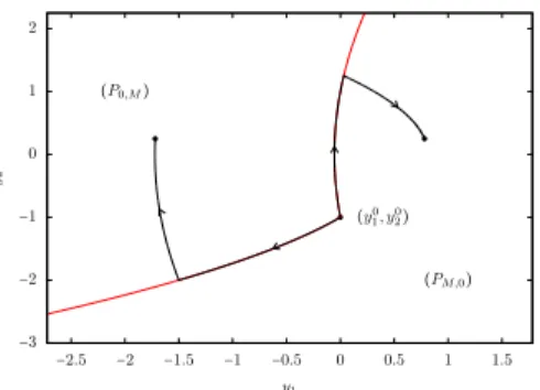
To compute the minimal time for this control problem, we add the control constraint w⩽ M with M destined to tend to+∞. According to [20, Theorem 20 p. 143], the time optimal control takes its values in{0, M} and has at most one switch. The following possible control strategies are given in Figure 2 for two types of initial conditions.
Taking the limit M→ ∞, we obtain:
1. if y20 > 0 and if the target (y11, y21) is different from the initial condition (y01, y02) then the minimal time required to reach the target with the control constraint w(t) ⩾ 0 is positive; 2. if y20 ⩽ 0, if the target (y11, y2) does not belong to the segment {y1 10} × [y20,−y02], then the
minimal time required to reach the target with the control constraint w(t) ⩾ 0 is positive, otherwise it is 0.
−3 −2 −1 0 1 2 3 4 −2 −1 0 1 2 3 4 5 6 (y0 1, y20) (P0,M) (PM,0) y2 y1
(a) Different types of optimal state trajectories with y0 2>0. −3 −2 −1 0 1 2 −2.5 −2 −1.5 −1 −0.5 0 0.5 1 1.5 (y0 1, y02) (P0,M) (PM,0) y2 y1
(b) Different types of optimal state trajectories with y0
2<0.
Figure 2: We take M = 10. The zones (P0,M) and (PM,0) are delimited by the red lines. When the target is in the zone(P0,M) (respectively (PM,0)), then the optimal control strategy is to take the control w equal to 0 and then M (respectively M and then 0). Examples of trajectories are plot in black.
Going back to the original system (2.8), we obtain that TC(y0, y1) can vanish if y1
1= y01and y21= y20 or if y11 = y10, y02 ⩽ 0 and y21∈ [y02,−y02]. Of course, due to the reduction procedure, we ignore the conditions on the last component y3 of y and at this step nothing ensures that the minimal time required to steer the original system from y0 = (y0
1, y02, y03)⊺ to y1 = (y11, y12, y13)⊺ is equal to the minimal time required to steer the reduced system from(y0
1, y02) ⊺ to(y1
1, y12) ⊺.
Let us also illustrate on this system, the condition given in the first point of the statement (ii) of Theorem 1.1 in order to have TC(y0, y1) = 0. More precisely, we give an example of initial and final conditions y0 and y1 such that y1− y0∈ Ran B (but do not fulfill the first point of statement (ii) of Theorem 1.1) and we show that TC(y0, y1) > 0. Namely, take y0= (0, 1, 0)⊺ and y1= (0, 1, 1)⊺. Let us prove that, if u∈ L∞(0, T ) is a classical L∞ control steering y0 to y1 in time T then we must have T ⩾ 1. This positive minimal time is due to the fact that y2(t) has to take some non-positive value. Indeed, assume by contradiction, that for every t∈ [0, T ], we have y2(t) > 0, then y1(T ) = ∫
T
0 y2(t) dt > 0, hence this control does not fulfill the target requirements. Consequently, there exists τ∈ [0, T ] such that y2(τ) ⩽ 0. But, since y2(t) = 1 + ∫0ty3(s) ds, and since y3(s) ⩾ −1, for every t> 0, we have y2(t) ⩾ 1 − t. Therefore, the first time instant τ such that y2(τ) ⩽ 0 cannot be lower than 1. This proves that TC(y0, y1) ⩾ 1.
Let us also notice that with a Dirac mass located at the initial time the target y1is instantaneously reached.
2.7
Additional comments
In Theorem 1.1, we only give the explicit minimal controllability time in the statement (i) and in the first point of statement (iii) and the minimal time is 0. When the assumption of the statement (i) is not completely satisfied (i.e. y1− y0∈ Ran B but there does not exist a steady state in {y0} + Ran B), then as we can see in the example above, the minimal time may be positive.
In the proof of Theorem 1.1, we show that the minimal controllability time TC(y0, y1) is non lower than the minimal controllability time of a reduced system with an unilateral
control constraint. Let us point out that nothing ensures that these two minimal times coincide. In particular, in the example above, we show that the minimal controllability time of the reduced system is zero for some well chosen terminal conditions, but the minimal controllability time TC(y0, y1) for the initial system is positive. Consequently, we cannot expect to have equality of the two times. Let us also mention that, in the only examples (showing this gap phenomenon) we have been able to build, the minimal controllability time for the reduced system is zero. Hence, we do not know if this gap appears in more general situations.
A problem that has not been tackled in this proof is the existence of a minimal time control. As we will see further in Proposition 4.1, generically there does not exist a classical L∞ control in time TC(y0, y1). However, we expect that a control exists in a wider class. If there exists a minimal time control for the reduced system, then a strategy to build a minimal time control would be to take as original control the Nth derivatives of the time optimal control for the reduced system (N being the number of Goh reductions that has been performed to obtain the reduced system). Of course, we expect that this control belongs to some space of distributions. To properly define a solution of the system with such irregular controls, we can use the transposition method (as done in [22]). In addition, with this control, the state might also be a distribution and we have to be careful with the definition of the state constraint y(t) ∈ C. However, when the state constraint is affine (as it is in the statement (iii) of Theorem 1.1), this should not be a problem.
One last point is that with this new irregular control, there is no reason that the terminal conditions be fulfilled. In particular, in the Brunovsky form, the last part of the state will not be reached. However, this might be overcome by adding some Dirac masses (and/or derivatives of Dirac masses) at the initial and final times.
The previous point is related with the following question: does the minimal time TC(y0, y1) defined with L∞ controls coincide with the minimal time defined with controls chosen in a wider class? To address this issue, a first step could be to consider Radon measure controls instead of L∞ controls, this ensures that the corresponding state trajectory belongs to L∞ and hence the state constraint y(t) ∈ C still makes sense. But as we can see in the example of Section 2.6, the target state(0, 1, 1)⊺can be reached instantaneously from the initial state (0, 1, 0)⊺ with a Dirac impulse whereas this requires a waiting time greater than 1 when using classical L∞ controls. Consequently, the minimal control time with Radon measure controls may differ from the minimal time with L∞controls. The study of conditions ensuring that these two minimal controllability times coincide is an interesting problem which would deserve more attention. We refer to [11, 30] for studies of a possible gap of the value functions respectively associated to classical L∞ controls or to relaxed measure controls.
3
Extensions of Theorem 1.1
3.1
Arbitrary unilateral state constraints
In the statement (iii) of Theorem 1.1, we have considered the unilateral affine state constraint (1.3). If, instead, we consider a nonlinear unilateral state constraint of the form c(y(t)) ⩾ 0 for some function c∶ IRn → IR of class C1, then the first and the second steps in Section 2 can be achieved as well.
Let us assume that m= 1 (only one scalar control) and let us be more precise. In the second step, Goh transformations are made until we come up with a mixed state and control constraint of the form c(z(⋅), v(⋅)) ⩾ 0, instead of the linear one in (2.6). To perform the third step, we assume
that ∂v∂c ≠ 0. Then, by the implicit function theorem, at least locally this constraint can be written in the form ϕ(z(⋅)) + v(⋅) ⩾ 0 (for some C1 function ϕ), and then one can set ¯v= ϕ(z) + v as a new control. But then, instead of (2.7), we obtain the new control system
˙
z(t) = Az(t) − bϕ(z(t)) + b¯v(t) = f(z(t)) + b¯v(t), ¯
v(⋅) ⩾ 0,
which is not linear anymore. The analysis done in the third step of Section 2 can still be done with only slight changes, in small time (replace etA with the flow etf). We do not provide details. We obtain here that, for generic functions c and for r= 1, there exists an open subset C1⊂ C such that TC(y0, y1) > 0 for every y1∈ C.
3.2
Nonlinear control-affine systems
Instead of considering the linear control system (1.2), we now consider the more general control-affine system ˙ y(t) = f(y(t)) + m ∑ i=1 ui(t)gi(y(t)), (3.1)
where f and the gj’s are smooth vector fields in IRn. We consider the optimal control problem of steering in minimal time the control system (3.1) from a given y0∈ C to some given y1 ∈ C, without control constraint but under the state constraint y(⋅) ∈ C.
Then the analysis done in Section 2 can still be performed with few changes under appropriate assumptions. There exist indeed nonlinear versions of the Brunovsky normal form: in [15], feedback equivalence with a linear control system is given under certain Lie bracket conditions (see also [1, 2]). Precisely, defining
Gi(y) = Span{adk
f.gj(y) ∣ k = 0, . . . , i, j = 1, . . . , m}
at any point y∈ IRn for i= 0, . . . , n − 1, it is stated in [15, Theorem 5.2.3 page 233] that if all Gi’s have constant dimension, if dim Gn−1= n and if Gi is involutive for i= 0, . . . , n−2 then there exists a (nonlinear) dynamic change of coordinates in which the system (3.1) can be written as a linear autonomous control system (1.2). This result is then applied in the first step of Section 2, the other steps are then unchanged.
We obtain that, for C bounded and, under the above Lie bracket assumptions, if y1− y0 ∉ G0(y0) then TC(y0, y1) > 0. This generalizes the statement (ii) of Theorem 1.1. We also obtain a generalization of the statement (iii), at least for r= 1 and for generic constraints as in Section 3.1. Finally, similarly to the statement (i) of Theorem 1.1, if there exists a steady state ¯y∈ ˚C such that the small time local controllability property holds at this point and if y0, y1 and ¯y belong to the interior of C and y1 and ¯y are in a same component of({y0} + G0(y0)) ∩ ˚C, then TC(y0, y1) = 0.
It is interesting to notice that, because of the involutivity assumption, the above conditions on the Lie brackets are (by far) nongeneric. They generalize the case of f(y) = Ay and gi(y) = bi∈ IRn. At the opposite, under the generic (in the sense of Whitney) condition that the Lie algebra Lie(g1, . . . , gm) generated by the vector fields gj is equal to IRn (Lie Algebra Rank Condition, also called Chow condition or H¨ormander assumption), we claim that TC(y0, y1) = 0 for all y0, y1∈ ˚C. Indeed, under this generating Lie bracket assumption (which requires that m> 1), given any path in IRn joining y0 to y1 and given any tubular neighborhood V of this path, one can find a control steering the system (3.1) from y0 to y1 in arbitrarily small time with a corresponding trajectory remaining in V (see, e.g., [16, Chapter 4]). This fact generalizes the statement (iii) of Theorem 1.1 for the case r> 1.
For m= 1 (only one scalar control), the situation is more complex. We have seen above that, under a nongeneric condition on the Lie brackets, the system is linearisable. But for generic vector fields(f, g1), the control system is not linearisable and actually new phenomena appear, which are typical of nonlinear systems. In particular, as soon as n⩾ 3, singular trajectories do occur in a generic way (see [1, 2]) and under an open condition they are moreover time optimal.
Let us be more precise. Assuming that n⩾ 3 and that m = 1, there always exists at least one singular trajectory y(⋅), “singular” meaning that the linearised control system along y(⋅) is not controllable. Now, along y(⋅) we make the following generic assumptions: the set K(t) = {adkf.g1(y(t)) ∣ k ∈ IN} is of codimension one in IRn and [g1,[g1, f]](y(t)) ∉ K(t) along the trajectory y(⋅). Under an additional sign condition meaning that the latter vector field points in a certain direction with respect to the hyperplane K(t), it is proved in [2, Chapter 10.8, Prop. 96] that there exists a tubular neighborhood of y(⋅) in which any minimal time trajectory is the concatenation of y(⋅) with some jumps at the initial and at the final time. In other words, such a trajectory steering the system from y0 to y1 has a first jump, at time t= 0, to join the curve y(⋅), then it follows the singular trajectory y(⋅) (and it must do so with a finite speed), and makes a final jump at the final time to reach the point y1.
It is noticeable that this structure is the one encountered in the turnpike phenomenon (see [29]). In any case, in this picture, time is lost along the singular trajectory. This is a new phenomenon with respect to the linear case where singular trajectories do not occur.
We summarize the above discussion in the following theorem. Theorem 3.1. Let C be a subset of IRn and let y0∈ C.
(i) Let y1∈ C ∖ {y0}. Assume that y0∈ ˚C and that there exists a point ¯y∈ ˚C at which small time local controllability holds. If ¯y and y1are in a same connected component of(y0+ G0(y0))∩ ˚C then TC(y0, y1) = 0.
(ii) Assume that C is bounded and let y1 ∈ C. If y1− y0 ∉ G0(y0), if dim Gi is constant for i = 0, . . . , n − 1, if dim Gn−1 = n and if Gi is involutive for i = 0, . . . , n − 2 (nongeneric assumptions) then TC(y0, y1) > 0.
(iii) Assume that Lie(g1, . . . , gm) = IRn(generic assumption, requiring that m> 1). Then TC(y0, y1) = 0 for all y0, y1∈ ˚C.
(iv) For m= 1 and n ⩾ 3, under generic assumptions on the vector fields, if the subset C con-tains singular curves then there exists an open set of terminal conditions (y0, y1) for which TC(y0, y1) > 0.
This theorem remains a bit informal but it is difficult to be more precise without entering into many technical considerations and this is not our aim here. As already explained, our main objective is to show that adding state constraints in an unconstrained control problem may create a positive minimal time.
4
Further facts
4.1
Steady-state controllability under state constraints
Definition 4.1. A point ¯y∈ C is a steady-state if there exists ¯u ∈ IRmsuch that A¯y+ B¯u = 0. For instance, when C= [0, +∞)n, a necessary and sufficient condition ensuring that any point of C is a steady-state is that
Ran B∩ Cone+(a1
where a1, . . . , an are the vectors of IRn that are the columns of A and Cone +
(a1, . . . , an) is the positive cone generated by these vectors.
Steady-states are particularly interesting because a connectedness assumption ensures that one can pass from any steady-state to any other one, while remaining in C, in large enough time. This assumption is the following:
Steady-state connectedness assumption:
Let y0 and y1 be two steady-states in ˚C. We assume that there exists a path of steady-states τ↦ ¯y(τ), 0 ⩽ τ ⩽ 1, such that ¯y(0) = y0 and ¯y(1) = y1 and such that ¯y(τ) ∈ ˚C for every τ∈ [0, 1].
Here, ˚C is the interior of C. Note that, since the system is linear, if C is convex then, given any steady-states y0 and y1 in ˚C, τ↦ ¯y(τ) = (1 − τ)y0+ τy1 is a path of steady-states contained in ˚C and thus the above steady-state connectedness assumption is satisfied.
Lemma 4.1. Under the Kalman condition (1.1) and under the steady-state connectedness as-sumption, given any two steady-states y0, y1 ∈ ˚C, there exist T > 0 (sufficiently large) and u ∈ L∞((0, T ), IRm) such that the corresponding solution y of (1.2) satisfies y(T ) = y1 and y(t) ∈ C for every t∈ [0, T ].
The proof consists of applying a local controllability argument (ensuring that the trajectory remains in C), repeatedly along the path of steady-states, and one gets the conclusion by compact-ness. We do not provide any details. Notice that, based on such arguments, quasi-static control strategies have been implemented in [8, 9] in view of controlling nonlinear heat and wave equations on steady-states. Let us also refer to [23] where this quasi-static control strategy has been used for the control of semi-linear heat equation under nonnegative state constraint.
4.2
No classical L
∞control at the minimal time
Proposition 4.1. Assume that either y0or y1 belongs to ˚C and that TC(y0, y1) ∈ (0, +∞). Then, exactly at T = TC(y0, y1), there does not exist any classical control u ∈ L∞((0, T ), IRm) steering the system (1.2) from y0 to y1 in time T .
This result ensures that the minimal time cannot be reached with L∞ controls as soon as the initial point or the target point is in the interior of the set of state constraints. One can easily build examples, where the minimal time is reached with L∞ controls. But this requires that the initial point and target point are in a same connected component of the boundary of the constraint set.
However, when y0 or y1 belong to ˚C, one can wonder whether the minimal time can be reached with impulse controls in the space of distributions. This issue has been discussed in Section 2.7. Proof. Reversing the time if necessary, we can assume that y0∈ ˚C. Let ε0 > 0 be such that the open ball B(y0, ε0) is contained in C.
Let us assume, by contradiction, that there exists a control u∈ L∞((0, TC), IRm) steering y0to y1. We set M= ∥u∥L∞. Let τ ∈ (0, TC] be such that ∥etA− In∥∣y0∣ + (M + 1)∥B∥ ∫
t 0 ∥e
(t−s)A∥ ds < ε0for every t∈ [0, τ]. The positive time instant τ is defined so that for every control u ∈ L∞((0, τ), IRm) satisfying ∥u∥L∞ ⩽ M + 1, the solution of (1.2) satisfies y(t) ∈ C for every t ∈ [0, τ]. We set
¯
y= y(τ; u), the solution at time τ of (1.2) with control u. Since u is assumed to be time optimal, it follows that τ is the minimal time required time to steer y0 to ¯y. Thus, u∣[0,τ ] is a minimal time control steering y0 to ¯y and we have∥u∣[0,t
0]∥L∞ ⩽ M < M + 1. Consequently, τ and u∣[0,τ ]
are also the minimal time and a time optimal control steering y0to ¯y under the control constraint ∥u∥L∞⩽ M + 1 (and without state constraint). But due to the saturation property (see [20]), any
time optimal control solution of the above time optimal control problem shall satisfy∥u∥L∞= M +1.
This contradicts the fact that u is a time optimal control.
4.3
Approximation of the minimal time function with control constraints
In order to systematically ensure existence of classical minimal time controls, we add the control constraint ∥u∥L∞ ⩽ M for some M > 0 (destined to be large). We define TCM(y0, y1) as the
minimal time required to steer the control system (1.2) from y0to y1 under the control constraint ∥u∥L∞⩽ M and under the state constraint C (with the agreement that TCM(y0, y1) = +∞ when y1
is not reachable from y0). We have TC(y0, y1) = T+∞ C (y
0, y1) and obviously we have TC(y0, y1) ⩽ TM
C (y
0, y1) and the function M ↦ TM C (y 0, y1) is nonincreasing. Proposition 4.2. lim M →+∞T M C (y 0 , y1) = TC(y0, y1).
Proof. We denote, in short, TC= TC(y0, y1) and TCM = TCM(y0, y1). Let us consider a minimizing sequence(Tn)n∈IN converging to TC, associated with controls un ∈ L∞((0, Tn), IRm) steering the system (1.2) to y1 in time Tn > 0 under the state constraint y(t) ∈ C. Set Mn = ∥un∥L∞. Since
TC ⩽ TMn C ⩽ Tn, it follows that T Mn C → TC as n→ +∞. Since T M C ⩽ TC Mn when 0< Mn⩽ M, the conclusion follows.
5
Explicit computations in 2D
In this section, we take n= 2 and m = 1 (B is a vector in IR2). The Brunovsky normal form for the control system (1.2) is then
˙
z1= z2, z2˙ = v, (5.1) with z = (z1, z2)⊺ = P−1y and v = F y + u, and with F = DA2, (P−1)⊺ = (D⊺ (DA)⊺) and D = (0 1)(B AB)−1. Steering (1.2) from y0 to y1 under the state constraint y(t) ∈ C is equivalent to steering (5.1) from z0= P−1y0 to z1= P−1y1 under the state constraint z(t) ∈ P−1C. For y0 and y1 two steady-states, z0 and z1 are two steady-states as well and thus zi = (z1i, 0)⊺ for i∈ {0, 1}. Consequently, without loss of generality, we aim to find the minimal controllability time in order to steer the system (5.1) from z0= (z0
1, 0)⊺ to z1= (z11, 0)⊺under the state constraint z(t) ∈ C. Let us define, for every ζ1∈ IR,
ϕ+(ζ1) =⎧⎪⎪⎨⎪⎪ ⎩
0 if(ζ1, 0)⊺∉ C, sup{ζ2∈ IR+ ∣ ∀ζ ∈ [0, ζ2], (ζ1, ζ)⊺∈ C} otherwise and similarly,
ϕ−(ζ1) =⎧⎪⎪⎨⎪⎪ ⎩
0 if(ζ1, 0)⊺∉ C, sup{ζ2∈ IR+ ∣ ∀ζ ∈ [−ζ2, 0], (ζ1, ζ)⊺∈ C} otherwise. The functions ϕ± can take the value+∞.
Proposition 5.1. Assume that C⊂ IR2 is a closed and simply connected set and z0= (z01, 0)⊺ and z1= (z11, 0)⊺ are two steady-states in C, such that the segment[z0, z1] belongs to the interior of C. Then TC(z0, z1) = ⎧⎪⎪⎪ ⎪⎪⎪ ⎨⎪⎪ ⎪⎪⎪⎪ ⎩ ∫ z10 z1 1 dζ ϕ−(ζ) if z11⩽ z10, ∫ z1 1 z0 1 dζ ϕ+(ζ) if z11⩾ z10.
Proof. Let us define ˜C as the closure of
{(ζ1, ζ2)⊺∈ IR2 ∣ ϕ+(ζ1) > 0, ϕ−(ζ1) > 0, −ϕ−(ζ1) < ζ2< ϕ+(ζ1)} .
Since ˜C⊂ C, we have TC˜(z0, z1) ⩾ TC(z0, z1) where TC˜(z0, z1) is the time required to steer (5.1) from z0 to z1 under the state constraint z(t) ∈ ˜C. Moreover, noting that if z2> 0 (resp., z2< 0) then z1 is increasing (resp., decreasing), a simple argument shows that any controlled trajectory in C steering z0= (z10, 0)⊺ to z1= (z1
1, 0)
⊺ remains in ˜C. Therefore, T ˜
C(z0, z1) = TC(z0, z1). Let us assume that z10< z11(the proof for the other case is similar). Considering the control system
˙
z1= z2with z2as a control subject to z2⩽ ϕ+(z1), we obtain TC(z0, z1) ⩽ ∫z
1 1 z0 1 dz2 ϕ+(z2). Let us prove the equality by using Proposition 4.2. For M> 0, we define the sets
˜ C+M = {(ζ 0 1+ T 2M/2 T M ) ∈ IR 2 ∣ T ⩾ 0, ζ0 1 ∈ IR s.t. ∀t ∈ [0, T ], ( ζ10+ t2M/2 tM ) ∈ ˜C} , ˜ C−M = {( ζ1 1− T2M/2 T M ) ∈ IR 2 ∣ T ⩾ 0, ζ1 1 ∈ IR s.t. ∀t ∈ [0, T ], ( ζ1 1− t2M/2 tM ) ∈ ˜C} , ˜ CM = ( ˜C+M∪ ˜C+−M) ∩ ( ˜C−M∪ ˜C−−M) .
In particular, we have ˜CM ⊂ ˜C and ˜CM contains all trajectories of (5.1) starting from a steady-state point and reaching a steady-steady-state point under the control constraint∣v(⋅)∣ ⩽ M and under the state constraint ˜C. Similarly to ϕ±, we define ϕM± and we check that ϕ
M
± (ζ) ⩽ ϕ±(ζ) and ϕM± (ζ) → ϕ±(ζ) as M → +∞ for every ζ ∈ IR. Furthermore, the minimal time T
M ˜ C (z
0, z1) required to steer the system (5.1) from z0to z1under the control constraint∣v(⋅)∣ ⩽ M and under the state constraint ˜C is∫z11 z0 1 dz2 ϕM +(z2)
. Taking the limit M→ +∞ gives the result.
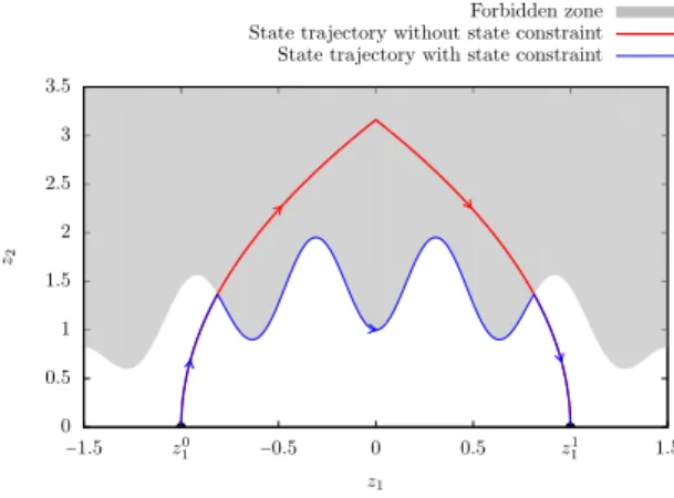
Remark 5.1. The minimal time control problem for the 2D system (5.1) under the state constraint z2(t) ∈ [−ϕ−(z1(t)), ϕ+(z1(t))] and under the control constraint ∣v(⋅)∣ ⩽ M can easily be solved when ϕ+and ϕ−are Lipschitz: given any M > 0 larger than the Lipschitz constants of ϕ+and ϕ−, the minimal time trajectory coincides with the minimal time trajectory without state constraint intersected with ∂C (see Figure 3). In other words: take the optimal solution without state constraint, truncate it with the allowed domain, and follow the lines.
The above comment is also valid when considering directly the control system (1.2) (for n= 2 and m = 1). More precisely, for a state constraint of order one, the minimal time trajectory between two steady-states, for the problem under state constraint and under control constraint ∣u(⋅)∣ ⩽ M with M > 0 sufficiently large, is exactly the optimal trajectory for the problem without state constraint, and constraint M on the control, ”intersected” with the authorized domain. This fact is however not true when n⩾ 3.
Example 5.1. Take A= (1 0 0 2), B= ( 1 1), y 0= ( 1 1/2), y 1= (2 1)
and the state constraints y1(⋅) ⩾ 0 and y2(⋅) ⩾ 0 (i.e., C = [0, +∞)2). Setting z = P−1y and v = (−1 4)y+u, with P−1= (−1 1
−1 2), we obtain the Brunovsky normal form (5.1) and the aim is to steer z0= P−1y0= (−1/2, 0)⊺ to z1= P−1y1= (−1, 0)⊺ under the state constraints z
2⩾ 2z1 if z1⩾ 0 and z2⩾ z1if z1⩽ 0. For every z1∈ IR, we compute ϕ+(z1) = 0 if z1> 0 and +∞ if z1< 0, and ϕ−(z1) = 0
0 0.5 1 1.5 2 2.5 3 3.5 z0 1 z11 −1.5 −0.5 0 0.5 1.5 z2 z1 Forbidden zone State trajectory without state constraint State trajectory with state constraint
Figure 3: Relations between the state trajectory with and without the state constraint and under the control constraint∣v(⋅)∣ ⩽ M.
−1 −0.8 −0.6 −0.4 −0.2 0 −1.1 −1 −0.9 −0.8 −0.7 −0.6 −0.5 −0.4 z2 z1 M= 1/2 M= 2 M= 100
(a) State trajectories in Brunovsky variables
−4 −2 0 2 4 0 0.5 1 1.5 2 v t M= 1/2 M= 2 M= 100
(b) Control in Brunovsky variables
0 0.2 0.4 0.6 0.8 1 0.4 0.6 0.8 1 1.2 1.4 1.6 1.8 2 x2 x1 M= 1/2 M= 2 M= 100
(c) State trajectories in initial variables
−4 −2 0 2 4 0 0.5 1 1.5 2 u t M= 1/2 M= 2 M= 100
(d) Control in initial variables
Figure 4: Minimal time trajectories steering y0 to y1 in Brunovsky variables (top) and in initial variables (bottom) for the state constraint problem, under the additional control constraint∣v(t)∣ ⩽ M , for M∈ {1/2, 2, 100}.
if z1> 0 and −z1 if z1⩽ 0. According to Proposition 5.1, we obtain TC(y0, y1) = ∫ −1 2 −1 dζ ϕ−(ζ) = ln 2 and TC(y1, y0 ) = ∫ −1 2 −1 dζ
ϕ+(ζ) = 0. On Figure 4, one can see a sequence of minimal time trajectories
ln 2 0 0.5 1 1.5 2 2.5 3 0 5 10 15 20 T M TM(z0, z1)
Figure 5: Convergence of the minimal time control with ∣v(t)∣ ⩽ M in Brunovsky variables, as M→ ∞.
under the control constraint∣v(⋅)∣ ⩽ M for M ∈ {12, 2, 100}, steering the system from y0 to y1. In accordance with Proposition 4.2, the corresponding sequence of minimal times converges to the minimal time given above. Simple computations show that, under the control constraint bound M , the minimal time is√2/M when M < 9/8 and√1+ 2/M −√1− 1/M + ln (
√ 1+2/M −1 1−
√
1−1/M) when M⩾ 9/8 (see also Figure 5).
Example 5.1 illustrates Proposition 5.1. The next example shows that the situation is more intricate when C is not simply connected.
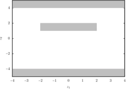
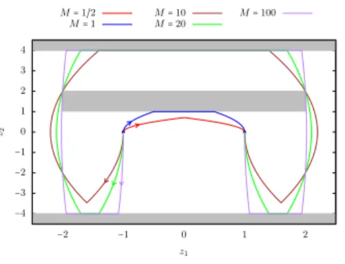
Example 5.2. We consider the set C drawn and defined by Figure 6, which is not simply connected. The objective is to steer the control system (5.1) from z0= (−1, 0)⊺ to z1= (1, 0)⊺ under the state
−4 −2 0 2 4 −4 −3 −2 −1 0 1 2 3 4 z2 z1
Figure 6: State constraint set considered in Example 5.2, the forbidden zones are in grey. constraint C. Proposition 5.1 would give the minimal time ∫−11 dζ2
1 = 2, but in fact the minimal time is∫−1−2dζ4 + ∫−22 dζ4 + ∫21dζ4 =32 (see Figure 7 to have an idea of this fact).
Optimal trajectories under the additional control constraint∣v(⋅)∣ ⩽ M are plotted on Figure 7. For M> 0 large enough, starting from z0= (−1, 0)⊺, the trajectory first goes to the left, then saturates
the constraint z2= −4, then goes to the right and grazes the obstacle in the middle, before hitting the constraint z2= 4 and following it for a while; and then, symmetrically to the final point.
−4 −3 −2 −1 0 1 2 3 4 −2 −1 0 1 2 z2 z1 M= 1/2 M= 1 MM= 10= 20 M= 100
Figure 7: Minimal time trajectories under the state constraints given in Figure 6, and under the additional constraint∣v(⋅)∣ ⩽ M, for M ∈ {12, 1, 10, 20, 100}.
6
Conclusion and further comments
We have shown that steering a finite-dimensional linear autonomous control system satisfying the Kalman condition, under state constraints but without control constraints, may require a positive minimal time, even for unilateral state constraints. We have proved that the positive minimal time phenomenon occurs for a bounded state constraint set, and more surprisingly, generically occurs for linear control systems as soon as there are more affine state constraints than controls (m⩽ k), but does not generically occur in the converse situation (m> k). We have extended our results to nonlinear control-affine systems, providing evidence that, when m= 1, the positive minimal time is rather due to the occurrence of singular trajectories, which is a typical nonlinear phenomenon.
Some remarks and open issues are in order.
We have shown that there does not exist any classical L∞ control realizing controllability exactly at the minimal time, but could we expect that there exists a control in the wider space of Radon measures. This is in particular the case for the heat equation with nonnegative Dirichlet controls (cf. [21]).
A problem related to the above point is the existence a gap between the minimal time obtained for the reduced system and the minimal time for the initial system. The example given in Section 2.6 indicates that such a gap may exist. But this example is very particular since the minimal time for the reduced system is zero. We point out that we did not find examples where a gap exists and the minimal time for the reduced system is positive. Explicit minimal times have been given for 2D systems (and lower bounds are given in [21]
for the heat equation). Obtaining such expressions, or at least, estimates, is an open problem in larger dimension.
The two latter items may certainly be addressed within impulsive optimal control theory (see [5, 6, 10, 26]). An open question is to investigate whether a version of the Pontryagin maximum principle, valid for Radon measures control, would allow one to provide evidence