Contribution à l'analyse de performance des robots parallèles

HAL Id: tel-01524856

https://hal.archives-ouvertes.fr/tel-01524856

Submitted on 19 May 2017

HAL is a multi-disciplinary open access archive for the deposit and dissemination of sci-entific research documents, whether they are pub-lished or not. The documents may come from teaching and research institutions in France or abroad, or from public or private research centers.

L’archive ouverte pluridisciplinaire HAL, est destinée au dépôt et à la diffusion de documents scientifiques de niveau recherche, publiés ou non, émanant des établissements d’enseignement et de recherche français ou étrangers, des laboratoires publics ou privés.

Contribution à l’analyse de performance des robots

parallèles

Ranjan Jha

To cite this version:

Ranjan Jha. Contribution à l’analyse de performance des robots parallèles. Robotique [cs.RO]. Ecole Centrale de Nantes (ECN), 2016. Français. �tel-01524856�

Ranjan JHA

Mémoire présenté en vue de l’obtention du

grade de Docteur de l’Ecole Centrale de Nantes

sous le label de L’Université Nantes Angers Le Mans

École doctorale : STIM

Discipline : Sciences pour l'ingénieur Unité de recherche : IRCCyN

Soutenue le 7 juillet 2016

Contributions to the performance

analysis of parallel robots

JURY

Rapporteurs : Jean-Pierre MERLET, Directeur de Recherche, INRIA

Grigore GOGU, Professeur, IFMA

Examinateurs :

Said ZEGHLOUL,Professeur, Université de Poitiers

Damien CHABLAT, Directeur de Recherche, CNRS Guillaume MOROZ, Chargé de Recherche, INRIA Fabrice ROUILLIER, Directeur de Recherche, INRIA

Invité(s) :

Directeur de Thèse : Damien CHABLAT, Directeur de Rercheche, CNRS

Ranjan JHA

Contributions to the performance analysis of parallel robots

Résumé

Cette thèse apporte des contributions pour plusieurs problèmes associés à la planification de mouvements pour les robots parallèles. Ces différents problèmes sont classis en quatre catégories: l’analyse de l'espace de travail et de l'espace articulaire ; les domaines d'unicité ; la planification des trajectoires et l'analyse de précision. L'analyse de l’espace de travail et de l'espace articulaire différencient les régions possédant un nombre constant de solutions aux modèles géométrique inverses et des directs en utilisant une décomposition algébrique cylindrique. Une méthode d’élimination utilisant des bases de Gröbner est utilisée pour calculer les singularités parallèles et sérielles des manipulateurs parallèles étudiés. Les surfaces caractéristiques sont également calculées pour définir les domaines d'unicité dans l'espace de travail. Une extension de la notion d’aspect est proposée pour les robots parallèles possédant plusieurs modes de fonctionnement, d’assemblage et d’opération. Une méthode algébrique est proposé pour vérifier la faisabilité de toutes les trajectoires données dans l'espace de travail pour régler le problème bien connu qui se pose lorsqu'il existe une configuration singulière entre les deux postures de la plate-forme mobile lorsque l’on discrétise la trajectoire avec une approche classique. Appliquée au robot NaVARo, un robot parallèle possédant plusieurs modes d'actionnement, une interface Matlab est présentée pour générer sa prise d’origine et ses mouvements en utilisant uniquement le modèle géométrique inverse. Pour l’Orthoglide 5-axes, une analyse de précision est réalisée pour estimer l'erreur de position de l’outil associée aux erreurs produites par la boucle de régulation PID. Le modèle d’erreur proposé, qui est basé sur les propriétés statiques et dynamiques de l’Orthoglide, permet d’estimer les erreurs de positionnement dans l'espace cartésien.

Mots clés

Manipulateur parallèles, planification des trajectoires, décomposition cylindrique algébrique, singularités, base de Gröbner, paramètres de conception, les indices de performance, modes d’opération

Abstract

This doctoral thesis focuses on the different aspects which are associated with efficient planning of desired tasks for parallel robots. These different aspects are mainly categorized in four parts, namely: workspace and joint space analysis, uniqueness domains, trajectory planning and accuracy analysis. The workspace and joint space analysis differentiate the regions with different number of inverse kinematic solutions and direct kinematic solutions using a

cylindrical algebraic decomposition algorithm,

respectively. The influence of design parameters and joint limits on the workspace boundaries for the parallel robots are reported. Gr\"{o}bner based elimination methods are used to compute the parallel and serial singularities of the manipulator under study. The descriptive analysis of a family of delta like robots is presented by using algebraic tools to induce the an estimation about the complexity in representing the singularities in the workspace and the joint space. The generalized notions of aspects and uniqueness domains are defined for the parallel robot with several operation modes. The characteristic surfaces are also computed to define the uniqueness domains in the workspace. An algebraic method is proposed to check the feasibility of any given trajectory in the workspace to address the well known problem which arises when there exists a singular configuration between the two poses of the end-effectors while discretizing the path with a classical approach. A Framework for the control loop of a parallel robot with several actuation modes is presented , which uses only the inverse geometric model. The accuracy analysis focuses on the estimation of errors in the pose of the end effector due to the joint's errors produced by the PID control loop. The proposed error model, which is based on the static and dynamic properties of the Orthoglide, helps in estimating the error in the Cartesian workspace

Key Words

Parallel manipulators, trajectory planning, cylindrical algebraic decomposition, singularities, Gröbner basis, design parameters, performance indices, operation modes

Acknowledgements

It is very well said that Solving a problem for which you know there’s an answer is like

climbing a mountain with a guide, along a trail someone else has laid. I would have never

been able to complete my dissertation without the guidance, help and support of the kind people around me, to only some of whom it is possible for me to give a particular mention here.

At every step God helped me not to waste the amazing opportunities that came before me and gave me confidence to utilize them. First of all, I would like to thank the almighty God for establishing me to complete this thesis. I would like to thank my parents, sister, brother-in-law and other family members for their support and great patience all the time. They have given me their unequivocal support throughout, as always, for which my mere expression of thanks likewise does not suffice.

My thesis at IRCCyN would not have been possible without the support, guidance and suggestions of many people. I would like to thank my thesis supervisors Prof. D. Chablat, Prof. F. Rouillier and Dr. G. Moroz, for giving me an opportunity to work with them.

I am deeply indebted to my research supervisor, Professor D. Chablat for presenting me such an interesting thesis topic. Each meeting with him added invaluable aspects to the implementation and broadened my perspective. He has guided me with his invaluable sug-gestions, lightened up the way in my darkest times and encouraged me a lot in the academic life. From him I have learned to think critically, to select problems, to solve them and to present their solutions.

I would like to address special thanks to the jury members, Prof. S. Zeghloul, Prof. J.P Merlet and Prof. G. Gogu for their valuable comments which helped to considerably im-prove the quality of the thesis.

I also thank robotics team, International Office members, my colleagues and lab mates at IRCCyN, Ecole Centrale de Nantes for being a constant source of motivation, enthusiasm and encouragement and making it a fun place to work at. I would like to extend my sin-cerest thanks to the European Commission for their generous fellowship (Erasmus Mundus INDIA4EU II) which allowed me to work on my thesis.

Résumé

Cette thèse apporte des contributions pour plusieurs problèmes associés à la planification de mouvements pour les robots parallèles. Ces différents problèmes sont classis en quatre catégories: l’analyse de l’espace de travail et de l’espace articulaire ; les domaines d’unicité ; la planification des trajectoires et l’analyse de précision. L’analyse de l’espace de travail et de l’espace articulaire différencient les régions possédant un nombre constant de solutions aux modèles géométrique inverses et directs en utilisant une décomposition algébrique cylin-drique. Une méthode d’élimination utilisant des bases de Gröbner est utilisée pour calculer les singularités parallèles et sérielles des manipulateurs parallèles étudiés. Les surfaces car-actéristiques sont également calculées pour définir les domaines d’unicité dans l’espace de travail. Une extension de la notion d’aspect est proposée pour les robots parallèles possédant plusieurs modes de fonctionnement, d’assemblage et d’opération. Une méthode algébrique est proposée pour vérifier la faisabilité de toutes les trajectoires données dans l’espace de travail a fin de régler le problème bien connu qui se pose lorsqu’il existe une configuration sin-gulière entre les deux postures de la plate-forme mobile lorsque l’on discrétise la trajectoire avec une approche classique. Appliquée au robot NaVARo, un robot parallèle possédant plusieurs modes d’actionnement, une interface Matlab est présentée pour générer sa prise d’origine et ses mouvements en utilisant uniquement le modèle géométrique inverse. Pour l’Orthoglide 5-axes, une analyse de précision est réalisée pour estimer l’erreur de position de l’outil associée aux erreurs produites par la boucle d’asservissement (PID). Le modèle d’erreur proposé, qui est basé sur les propriétés statiques et dynamiques de l’Orthoglide, permet d’estimer les erreurs de positionnement dans l’espace cartésien.

Mots-clés: Manipulateur parallèles, planification des trajectoires, décomposition cylindrique algébrique, singularités, base de Gröbner, paramètres de conception, modes d’opération.

Abstract

This doctoral thesis focuses on the different aspects which are associated with efficient plan-ning of desired tasks for parallel robots. These different aspects are mainly categorized in four parts, namely: workspace and joint space analysis, uniqueness domains, trajectory planning and accuracy analysis. The workspace and joint space analysis differentiate the regions with different number of inverse kinematic solutions and direct kinematic solutions using a cylindrical algebraic decomposition algorithm, respectively. The influence of design parameters and joint limits on the workspace boundaries for the parallel robots are reported. Gröbner based elimination methods are used to compute the parallel and serial singularities of the manipulator under study. The descriptive analysis of a family of delta like robots is presented by using algebraic tools to induce an estimation about the complexity in repre-senting the singularities in the workspace and the joint space. The generalized notions of aspects and uniqueness domains are defined for the parallel robot with several operation modes. The characteristic surfaces are also computed to define the uniqueness domains in the workspace. An algebraic method is proposed to check the feasibility of any given tra-jectory in the workspace to address the well known problem which arises when there exists a singular configuration between the two poses of the end-effectors while discretizing the path with a classical approach. A Framework for the control loop of a parallel robot with several actuation modes is presented , which uses only the inverse geometric model. The accuracy analysis focuses on the estimation of errors in the pose of the end effector due to the joint’s errors produced by the PID control loop. The proposed error model, which is based on the static and dynamic properties of the Orthoglide, helps in estimating the error in the Cartesian workspace.

Keywords: Parallel Robots, Trajectory Planning, Cylindrical Algebraic Decomposition, Singularities, Gröbner Basis, Design Parameters, Operation Modes, Workspace.

Contents

Acknowledgements

i

Résumé

iii

Abstract

v

Nomenclature

1

Introduction

3

I Definitions and Mathematical Tools

11

I.1 Parallel Robots

· · · ·

I.1.1 Create Manipulator with SIROPA · · · ·12

I.1.2 Workspace and Jointspace · · · ·12

I.2 Kinematics : IKP and DKP

· · · ·

I.3 Singularities

· · · ·

I.3.1 Parallel Singularities · · · ·17

I.3.2 Serial Singularities · · · ·18

I.4 Assembly modes and Working modes

· · · ·

I.5 Operation Modes

· · · ·

I.6 Aspects and Uniqueness Domains

· · · ·

I.6.1 Aspect for parallel manipulators with single IKS · · · ·21

I.6.2 Aspect for parallel manipulators with multiple IKS · · · ·21

I.6.3 Characteristic surfaces· · · ·21

I.6.4 Basic components and Basic regions · · · ·22

viii

I.7 Non-Singular assembly mode changing trajectories

· · · ·

I.8 Standard Bases (Gröebner Bases)

· · · ·

I.9 Discriminant Variety and Cylindrical Algebraic Decomposition

· · · ·

I.10 Conclusions

· · · ·

II Workspace and Joint Space Analysis

31

· · · ·

II.2 Manipulators Under Study

· · · ·

II.2.1 Orthoglide Architecture and Kinematics · · · ·32

II.2.2 Hybridglide Architecture and Kinematics · · · ·33

II.2.3 Triaglide Architecture and Kinematics· · · ·33

II.2.4 UraneSX Architecture and Kinematics· · · ·34

II.2.5 Reconfigurable 3-RPS Parallel Robot · · · ·35

II.2.6 NaVARo 3RRR Planar Parallel Robot · · · ·38

II.3 Workspace Analysis of a Delta-like Family Robot

· · · ·

II.4 Joint space Analysis of a Delta-like Family Robot

· · · ·

II.5 Workspace Analysis of the 3RPS Parallel robot

· · · ·

II.5.1 Operation Modes · · · ·42

II.5.2 Cylindrical Algebraic Decomposition · · · ·43

II.5.3 Workspace: 3T Projection Space for OM1 and OM2 · · · ·44

II.6 Joint space Analysis of the 3RPS Parallel robot

· · · ·

II.7 Conclusions

· · · ·

III Aspects and Uniqueness Domains

51

· · · ·

III.2 Singularities: Delta-Like Family Robot

· · · ·

III.2.1 Parallel Singularities: Projection in workspace and jointspace · · · ·52

III.2.2 Serial Singularities: Projection in workspace and jointspace· · · ·54

III.2.3 Complexity in Singularities · · · ·56

III.3 Parallel Singularies of 3RPS Parallel robot

· · · ·

III.4 Influence of design parameter on Parallel Singularities

· · · ·

III.5 Aspect for an Operation mode

· · · ·

III.6 Characterstic surfaces for an operation mode

· · · ·

III.7 Uniqueness domains

· · · ·

III.8 Non Singular assembly mode Trajectories

· · · ·

III.9 Conclusions

· · · ·

IV Trajectory Planning

71

· · · ·

IV.2 Methodology

· · · ·

IV.3 Method Validation

· · · ·

IV.3.1 Manipulator Architecture and Kinematics · · · ·75

IV.3.2 Trajectory definition in the workspace· · · ·78

IV.3.3 Projection in the joint space · · · ·79

ix

IV.4 Parallel Manipulator with Several Actuation Modes

· · · ·

IV.4.1 Robot under study · · · ·86

IV.4.2 Transmission System · · · ·87

IV.4.3 Control Hardware and Software · · · ·88

IV.4.4 Sensor Placements· · · ·88

IV.4.5 Graphic user interface · · · ·89

IV.5 Homing

· · · ·

IV.5.1 Introduction · · · ·89

IV.5.2 Direct kinematics of the 3-RPR · · · ·89

IV.5.3 Direct kinematics of the 3-RRR · · · ·90

IV.5.4 Homing procedure · · · ·91

IV.6 Motions of the robot

· · · ·

IV.6.1 Inverse kinematic model · · · ·92

IV.6.2 Jacobian matrices· · · ·94

IV.6.3 Actuation mode changing· · · ·95

IV.6.4 Motions of the robot · · · ·95

IV.7 Conclusions

· · · ·

V Prospective Work: Evaluation of the Accuracy

97

· · · ·

V.2 Architecture & Kinematics: Orthoglide 5-AXIS

· · · ·

V.2.1 Direct Kinematics Model:· · · ·99

V.2.2 Inverse Kinematics Model: · · · 100

V.2.3 Parallel Singularities · · · 101

V.3 Trajectory Planning

· · · ·

V.4 Error Analysis

· · · ·

V.5 Error Model

· · · ·

V.6 Projection of Joint Errors in the Workspace

· · · ·

V.7 Influence of Starting positions on the joints errors

· · · ·

V.7.1 Joints errors for different starting positions · · · 111

V.7.2 Projection of Joint errors in the Cartesian space · · · 116

V.8 Conclusions

· · · ·

VI Conclusions and Future Work

119

· · · ·

VI.2 Main Contributions

· · · ·

VI.3 Future Work

· · · ·

Personal Publications

125

A Appendix Mathematical Expressions

127

· · · ·

A.2 Parallel Singularities

· · · ·

A.3 Serial Singularities

· · · ·

A.4 Reconfigurable 3RPS Parallel Robot

· · · ·

B Appendix SIROPA Library

139

· · · ·

x

C Appendix Timeline

149

List of Figures

I.1 Projection of parallel Singularity curves . . . 17

I.2 Projection of serial Singularity curves . . . 18

I.3 Assembly modes of orthoglide . . . 19

I.4 Postures of orthoglide . . . 19

I.5 Octree model of the characterstic surfaces . . . 22

I.6 Octree model of the basic regions . . . 23

I.7 Octree model of the basic components . . . 23

I.8 Octree model of the uniqueness domain . . . 24

I.9 Non-singular assembly-mode changing trajectory . . . 25

II.1 Configuration plot for Orthoglide robot . . . 33

II.2 Configuration plot for Hybridglide robot . . . 33

II.3 Configuration plot for Triaglide robot . . . 34

II.4 Configuration plot for UraneSX robot . . . 34

II.5 3-RPS parallel robot . . . 35

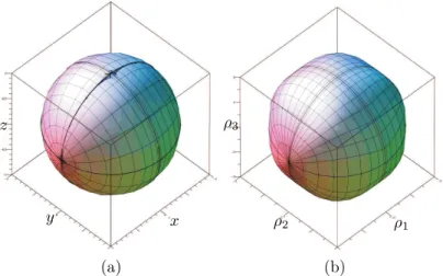
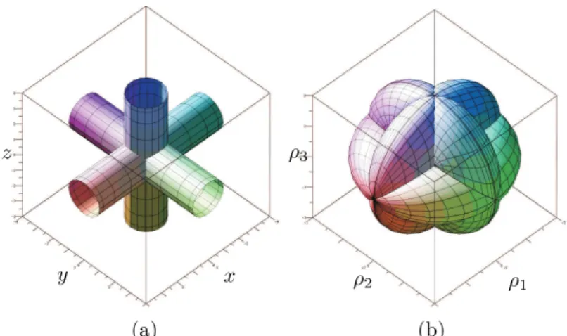
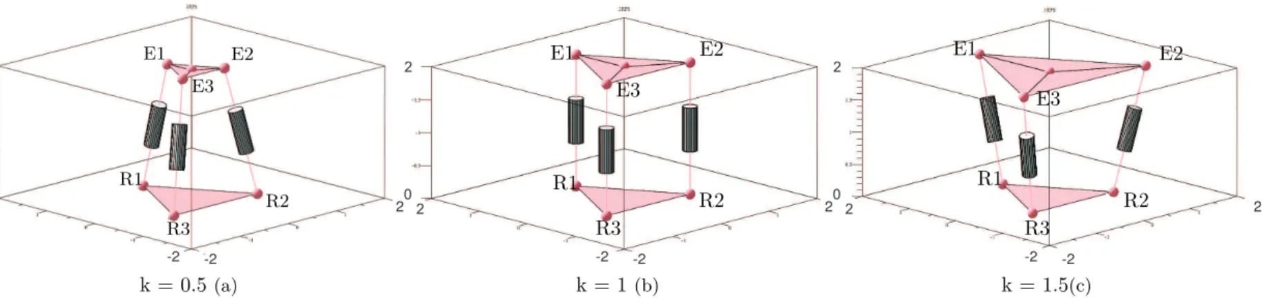
II.6 Virtual model of 3-RPS parallel manipulator with different design parameter k, k = 0.5 (a), k = 1 (b), k = 1.5 (c) . . . 36

II.7 The NaVARo robot . . . 38

II.8 The virtual model of the NaVARo robot . . . 38

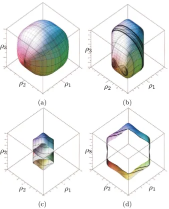
II.9 Workspace plot for delta robots . . . 39

II.10 Jointspace plot for delta robots . . . 41

II.11 Aspects for OM1 _{with det(A) < 0 (a) and det(A) > 0 (b) and aspects for} OM2 _{with det(A) < 0 (c) and det(A) > 0 (d) . . . 42}

xii

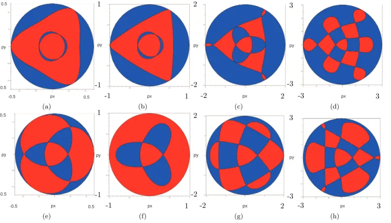
II.12 Slice of workspace for OM1 _{with different design parameter and p}

z= 2, k =

0.5 (a), k = 1 (b), k = 2 (c) and k = 3 (d) for OM2 k = 0.5 (e), k = 1 (f), k = 2 (g) and k = 3 (h). Blue and red regions corresponds to the four number

of solutions for the IKP for det(A) > 0 and det(A) < 0, respectively. . . 45

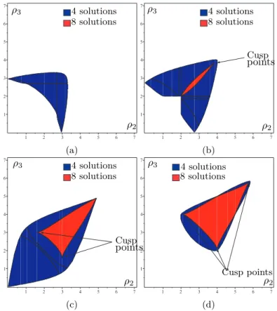
II.13 Slice of the joint space for ρ1= 3 . . . 46

II.14 Slice of the joint space for OM1 _{for different values of ρ . . . 46}

II.15 Cusp points for OM1 _{and OM}2 _{. . . 46}

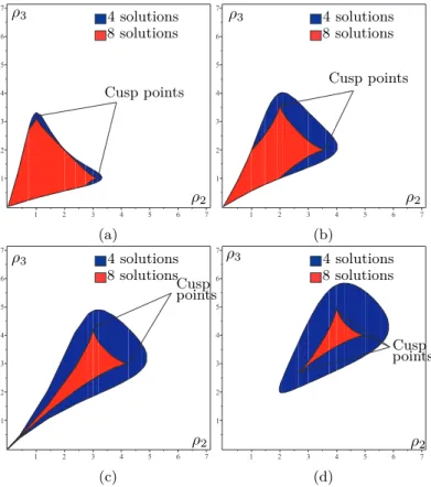
II.16 Slice of the joint space for ρ1 = 1, k = 0.5 (a), ρ1 = 1, k = 1 (b), ρ1 = 1, k = 1.5 (c), ρ1= 2, k = 0.5 (d), ρ1 = 2, k = 1 (e), ρ1= 2, k = 1.5 (f), ρ1= 3, k = 0.5 (g), ρ1 = 3, k = 1 (h) ρ1 = 3, k = 1.5 (i), where the DKP admits four, eight, twelve and sixteen real solutions in the blue, red, yellow and pink region, respectively. . . 47

II.17 Slice of the joint space for OM2 _{for different values of ρ . . . 48}

III.1 Projection of parallel singularity curve in workspace . . . 53

III.2 Projection of parallel singularity curve in jointspace . . . 54

III.3 Projection of serial singularity curve in jointspace . . . 55

III.4 Projection of serial singularity curve in workspace . . . 55

III.5 Singularity curves and its 2D projection for q1 = 0 . . . 58

III.6 Singularity curves and its 2D projection for q4 = 0 . . . 58

III.7 Projection of parallel singularities in projection space [px, py, pz] for OM1. Variation in the parallel singularities surface for different design parameter k = 0.5 (a), k = 1 (b), k = 2 (c) and k = 3 (d), top view of the parallel singularities surface, k = 0.5 (e), k = 1 (f), k = 2 (g) and k = 3 (h). . . 59

III.8 Projection of parallel singularities in projection space [px, py, pz] for OM2. Variation in the parallel singularities surface for different design parameter k = 0.5 (a), k = 1 (b), k = 2 (c) and k = 3 (d), top view of the parallel singularities surface, k = 0.5 (e), k = 1 (f), k = 2 (g) and k = 3 (h). . . 60

III.9 Aspects for OM1 _{and OM}2 _{. . . 61}

III.10Singularity curves and characteristic surfaces with z = 3 for OM1 _{(a) OM}2 _{(b) . 62} III.11Slice of an aspect for z = 3 and OM1 for det(A) > 0 and det(A) < 0 . . . 63

III.12Slice of an aspect for z = 3 and OM2 _{for det(A) > 0 and det(A) < 0 . . . 64}

III.13Basic regions of OM1 _{for det(A) > 0 . . . 64}

III.14Basic regions of OM1 _{for det(A) < 0 . . . 65}

III.15Basic regions of OM2 _{for det(A) > 0 . . . 66}

III.16Basic region of OM2 for det(A) < 0 . . . 67

III.17Slice of an aspect for z = 3 and det(A) > 0 for OM1 _{(a) OM}2 _{. . . 68}

III.18Variation of det(A) along trajectory for OM1 _{and OM}2 _{. . . 68}

III.19Projection in Q of the trajectories with the cusp curves . . . 69

IV.1 Architecture of an Orthoglide including two assembly modes (a) Workspace plot with χ(ρ) joint constraints (b) and Parallel singularity det(A) projected in the workspace as ξ(X) (c) and joint space plot with χ(ρ) joint limits (d) . . . 76

IV.2 A comparison between the parallel singularity surface for an Orthoglide com-puted with the joint limits µ(X) (a) without µ(X) (b) . . . 77 IV.3 Position of Trajectories 1&2 (a) Trajectory 3 (b) in the workspace of an Orthoglide78

xiii

IV.4 A pictorial representation of the mapping of trajectories from workspace to joint space. Eight different pairs of trajectories, Υ1(ρ, t) & Υ2(ρ, t) in joint

space are the image of corresponding φ1(t) & φ2(t). These eight different

trajectories are associated with the eight working modes of the Orthoglide. Only one trajectory lies inside the joint space boundary due to to the joint

constraints. . . 79

IV.5 Mapping of the Trajectory 3 from workspace to joint space. Eight different possible solutions of Υ3(ρ, t) are marked in joint space which are the image of φ3(t). There is only one feasible trajectory (marked as 1) lies inside the joint space boundary. . . 80

IV.6 Representation of the trajectories with singularity surface. Trajectory 1 cuts the parallel singularity surface ξ(X) in four points s1, s2, s3 and s4 in the workspace of the Orthoglide. Also, it can be seen that Trajectory 2 lies inside ξ(X) as µ2(t)6= 0 ∀t ∈ [−π, π]. . . 82

IV.7 Representation of the real singular points s3and s4along with the singularity surface ξ(X), which is associated with one working mode. . . 83

IV.8 Variation of µ1(t) along Trajectory 1. s1, s2, s3 and s4 represents the four solutions of µ1(t) = 0 ∀t ∈ [−π, π]. . . 83

IV.9 Variation of det(A) along the Trajectory 1. s3 and s4 represents the two solutions of det(A) = 0 _{∀t ∈ [−π, π]. . . 84}

IV.10Variation of µ2(t) along the Trajectory 2. There are no solutions for µ2(t) = 0 _{∀t ∈ [−π, π]. . . 85}

IV.11Variation of µ3(t) along the Trajectory 3. There are no solutions for µ3(t) = 0 _{∀t ∈ [−π, π]. . . 85}

IV.12The NaVARo robot . . . 86

IV.13The virtual model of the NaVARo robot . . . 87

IV.14The NaVARo transmission system . . . 87

IV.15The graphic user interface of the NaVARo robot . . . 89

IV.16Joint space of 3RPR parallel mechanism (a) without joint limits (b) with joint limits. The Red and Blue regions represents the two and four real solutions for the DKP, respectively. . . 90

IV.17First assembly mode of the NaVARo shown with pink colored mobile platform and the second assembly mode shown with yellow colored mobile platform for θ1=−0.585, θ2 =−2.680 and θ3 = 1.508 . . . 91

IV.18Flow chart of the control loop . . . 92

IV.19Definition of the angles used to solve the inverse kinematics . . . 93

V.1 Semi industrial prototype of the Orthoglide 5-Axis . . . 99

V.2 Simplified architecture of the Orthoglide for the simulation and the analysis. . . 100

V.3 Location of the trajectories φi(t) along with the parallel singularity surfaces ξ(X). CAD algorithm is used to plot these surfaces for a single working mode. . 102

V.4 Cartesian velocities along the trajectories φi(t) . . . 103

V.5 Cartesian acceleration along the trajectories φi(t) . . . 103

V.6 Joint parameters values along trajectories φ1(t), φ2(t), φ3(t), φ4(t), φ5(t) Joint positions (ai) Joint velocities (bi) Joint accelerations (ci), where i = 1, 2, 3, 4, 5 which represents different trajectories . . . 104

V.7 Joint errors in ∆ρ1 (a) ∆ρ2 (b) and ∆ρ3 (c) along the trajectories φi(t), Experimental data from the Orthoglide 5-axis . . . 107

xiv

V.8 Joint error ∆ρi and proposed error model ∆ρim value along trajectory φ1(t):

[−80, −80, −140], φ2(t): [−80, −80, −80], φ3(t): [00, 00, 00], φ4(t): [80, 80, 140],

φ5(t): [80, 80, 140] ∆ρ1(ai)∆ρ2 (bi) ∆ρ3 (ci), where i = 1, 2, 3, 4, 5 which

rep-resents different trajectories . . . 108 V.9 Cartesian errors in x (a) y (b) and z (c) along the trajectories φi(t), Image

of the joint errors in the workspace of the manipulator . . . 110 V.10 Different starting points on the trajectory to analyse the influence on the

accuracy of the Orthoglide. . . 112 V.11 Joint error values, ∆ρj from experimental data for different starting position

[Ti: [0] (in blue), Ti : [π/2] (in green), Ti: [π] (in red), Ti : [3π/2] (in black)]

of Orthoglide 5-axis along trajectories φ1(t), φ2(t), φ3(t), φ4(t), φ5(t) for ρ1

(a) ρ₂ (b) ρ₃ (c), where i = 1, 2, 3, 4, 5 which represents different trajectories

and j = 1, 2, 3. . . . 113 V.12 Cartesian velocities, ˙ρi (ai) and Cartesian accelerations, ¨ρi (bi) along

trajec-tory φ5(t) for different starting positions [T5 : [0] (in blue), T5 : [π/2] (in

green), T5: [π] (in red), T5 : [3π/2] (in black)]. . . 116

V.13 Cartesian errors in x (a1), y (a2), z (a3) and norm (a4) along the trajectories

φ5(t) for different starting positions [T1 : [0] (in blue), T2 : [π/2] (in green),

T3 : [π] (in red), T4 : [3π/2] (in black)], Image of the joints errors in the

workspace of the manipulator. . . 117 V.14 Cartesian errors, norm, along trajectories φ1(t) (a1), φ2(t) (a2), φ3(t) (a3),

φ4(t) (a4) and φ5(t) (a5) for different starting positions [T1 : [0] (in blue),

T₂ : [π/2] (in green), T₃ : [π] (in red), T₄ : [3π/2] (in black)], Image of the

joints errors in the workspace of the manipulator. . . 117 VI.1 Parallel singularity surface of 3RPS parallel robot (a) The methodology can

be extended to find the optimized path between point p1 and p2(b) which is

shown in red color. . . 123 VI.2 The virtual model of the 3RRR robot . . . 124

List of Tables

I.1 Description of the fields of CreateManipulator function . . . 13

I.2 Description of the fields of CellDecompositionPlus function . . . 15

I.3 Description of the fields of DiscriminantVariety function . . . 27

I.4 Description of the fields of CellDecomposition function . . . 29

II.1 Definition of the Workspace with CAD . . . 40

II.2 Definition of the Jointspace with CAD . . . 40

III.1 Comparison of the different parameters associated with the parallel singular-ities for the robots . . . 56

III.2 Comparison of the different parameters associated with the serial singularities for the robots . . . 57

III.3 Solutions of the DKP for det(A) > 0 . . . 68

IV.1 Singular postures on Trajectory 1 . . . 84

IV.2 The eight actuation modes of the NaVARo . . . 88

V.1 The Minimum, Maximum and mean absolute values of joint errors along the trajectories . . . 106

V.2 Maximum and mean absolute values of Cartesian position errors . . . 109

V.3 The Minimum, Maximum and mean absolute values of joint errors along the trajectories with different starting position . . . 114

B.1 Different Functions for Analysing in SIROPA . . . 139

B.2 Different Functions for Modeling in SIROPA . . . 140

B.3 Different Functions for Plotting in SIROPA . . . 140

xvi

B.5 Different Functions for Extra Algebra . . . 147 B.6 Different Functions for Trigonometric . . . 147

Nomenclature

ASME American Society of Mechanical Engineers

IFToMM International Federation for the Promotion of Mechanism and Machine Science

PM Parallel Manipulator(s)

PID Proportional Integral Derivative CAD Cylindrical Algebraic Decomposition

3T Three Translational Motion

2R1T Two Rotational and one Translational Motion

IKP Inverse Kinematics problem

DKP Direct Kinematics problem

det Determinant

OM Operation Mode

R Revolute Joint

P Prismatic Joint

S Spherical Joint

WA Aspect of the Operation mode

Sc Characteristic surfaces

WAb Basic Regions

QA Basic Components

ρ Actuated Joint Variables

X Pose Variables

Ψ System of Equations

Υ Projections in Joint space

A Direct kinematics Jacobian matrices

B Inverse kinematics Jacobian matrices

ξ(X) Projections of the parallel singularities in the Workspace

ε(ρ) Projections of the parallel singularities in the joint space

χ(ρ) Joint limits of the actuator

Introduction

Motivation

Robots have been a reality on factory assembly lines for over twenty years. A revolution in the field of robotics transforms the global economy for past few years, cutting the costs of services for the people. The researchers and engineers across the world made remarkable contributions for the efficient use of robots in the manufacturing, health, entertainment and aeronautical sectors.This doctoral thesis focuses on the different aspects which are associ-ated with efficient planning of desired tasks for parallel robots. These different aspects are mainly categorized in four parts, namely: workspace and joint space analysis, uniqueness domains, trajectory planning and accuracy analysis. The workspace and joint space analy-sis differentiate the regions with different number of inverse kinematic solutions and direct kinematic solutions using a cylindrical algebraic decomposition algorithm, respectively. The influence of design parameters and joint limits on the workspace boundaries for the parallel robots are reported. Gröbner based elimination methods are used to compute the parallel and serial singularities of the manipulator under study. The descriptive analysis of a fam-ily of delta like robots is presented by using algebraic tools to induce an estimation about the complexity in representing the singularities in the workspace and the joint space. The generalized notions of aspects and uniqueness domains are defined for the parallel robot with several operation modes. The characteristic surfaces are also computed to define the uniqueness domains in the workspace. An algebraic method is proposed to check the feasi-bility of any given trajectory in the workspace to address the well known problem which arises when there exists a singular configuration between the two poses of the end-effectors while discretizing the path with a classical approach. A Framework for the control loop of a parallel robot with several actuation modes is presented , which uses only the inverse geometric model. The accuracy analysis focuses on the estimation of errors in the pose of the end effector due to the joint’s errors produced by the PID control loop. The proposed error model, which is based on the static and dynamic properties of the Orthoglide, helps in estimating the error in the Cartesian workspace.

The workspace can be defined as the volume of space of the complete set of poses which the end-effector of the manipulator can reach. Many researchers published several works on the problem of computing these complete sets for robot kinematics. Based on the early studies [1, 2], several methods for workspace determination have been proposed, but many of them are applicable only for a particular class of robots. The workspace of parallel robots

4

mainly depends on the actuated joint variables, the range of motion of the joints and the mechanical interferences between the bodies of mechanism. There are different techniques based on geometric [3,4], discretization [5,7,8], and algebraic methods [9,10,11,12] which can be used to compute the workspace of parallel robot. The main advantage of the geo-metric approach is that, it establish the nature of the boundary of the workspace [19]. Also it allows to compute the surface and volume of the workspace while being very efficient in terms of storage space, but when the rotational motion is included, it becomes less efficient. Interval analysis based methods can be used to compute the workspace but the com-putation time depends on the complexity of the robot and on the requested accuracy [8]. Discretization methods are usually less complicated and can easily take into account all kine-matic constraints, but they require more space and computation time for higher resolutions. The majority of numerical methods which is used to determine the workspace of parallel manipulators includes the discretization of the pose parameters for computing workspace boundaries [7]. There are other approaches, which are based on optimization algorithms [20] for fully serial or parallel manipulators, analytic methods for symmetrical spherical mecha-nisms [21].

Algebraic methods are used in [12, 11, 14, 22, 23,24] to study planar or spatial parallel robots. Two main steps are necessary to perform the workspace and joint space analysis. First, the discriminant variety is computed to characterize the boundaries of the workspace and joint space as well as the singularities. Second, the Cylindrical Algebraic Decomposition is used to define the connected regions where there exists a constant number of real solutions to the inverse or direct kinematic problem and no parallel or serial singularities [12, 14,15]. A cylindrical algebraic decomposition based method is illustrated in [11, 16], which is used to model the workspace and joint space for the 3 RPS parallel robot. The workspace analysis for the 3RPS and delta-like family parallel manipulators are presented in a chapter of the thesis. The cylindrical algebraic decomposition method and Gröbner based computations are used to model the workspace in 3T & 2R1T projection spaces, where the orientation of the mobile platform is represented by using quaternions. A certified three dimensional plot-ting is proposed to study the shape of the workspace for different delta like manipulators. This thesis presents the results which are obtained by applying algebraic methods for the workspace and joint space analysis of a family of delta-like robot including complexity in-formation for representing the singularities in the workspace and the joint space. The CAD algorithm is used to study the workspace and joint space, and a Gröbner based elimination process is used to compute the parallel and serial singularities of the manipulator.

For the design or the trajectory planning, the workspace of the parallel manipulator is divided into singularity-free regions [17]. The singularities divide the workspace into aspects and the characteristic surfaces induce a partition of each aspect into a set of regions (the basic regions) [18]. For the parallel robots with several inverse and direct kinematic solu-tions, the aspects are defined as the maximal singularity-free sets in the workspace or in the

5

cross-product of the joint space by the workspace. An assembly mode is associated with a solution for the Direct Kinematic Problem and a working mode for the Inverse Kinematic Problem (IKP). Practically, a change of assembly mode may occur during the execution of a trajectory between two configurations in the workspace which are not necessarily associated with the same input for a given working mode. The uniqueness domains can be defined as the maximal regions of the workspace where all the displacements of the end-effector can be accomplished without changing of assembly mode and working mode [12].

One of the crucial steps in the trajectory planning is to check the singularity-free paths in the workspace for the parallel manipulators. It becomes a necessary protocol to validate the trajectory when the parallel robot is used in practical applications such as precise man-ufacturing operations. A trajectory verification problem is presented in [25], based on some validity criteria like whether the trajectory lies fully inside the workspace of the robot and is singularity-free. Singularity-free path planning for the Gough-Stewart platform with a given starting pose and a given ending pose has been addressed in [26] using the clustering algorithm is presented in [27]. An exact method and an approximate method are described in [28] to restructure a path close to the singularity locus into a path that avoids it while remaining close to the original path. Due to the geometry of the mechanism, the workspace may not cover fully the space of poses [27], hence it is necessary to analyze the workspace of the manipulator. A procedure to automatically generate the kinematic model of parallel mechanisms which further used for singularity free path planning is reported in [30]. An algo-rithm for computing singularity-free paths on closed-chain manipulators is presented in [31], also this method attempts to connect the given two non-singular configurations through a path that maintains a minimum clearance with respect to the singularity locus at all points. The main drawback of numerical or discretization methods is that there might be a sin-gular configuration between two poses of the end-effectors when discretizing the path. This thesis illustrates a technique based on some algebraic methods to check the feasibility of any given trajectory in the workspace : it allows to write the Jacobian of the manipulator as a function of the time and to check whether its determinant vanishes between two poses. Also, when the trajectory meets a singularity, its location can also be computed.

The accuracy to reach the exact pose for the parallel manipulator for a given trajectory depends on the static and dynamic parameters associated with the manipulator. Due to their better dynamic properties, high load-carrying capacity, high accuracy and stiffness, closed loop mechanisms are best suited for the medical robotics, high-precision and machine tool design applications. Number of links and passive joints in the closed loop mechanism reduce the accuracy of the manipulator. There are different factors which affect the accuracy of the manipulator, some of them are geometrical deviations of the machine parts during their as-sembly, mechanism motions, elastic deformations of the links and joints due to the force and thermal expansion [32, 33]. There are several article exists on the effect of manufacturing tolerances on the accuracy of the parallel manipulators [34]. In [35], a forward and inverse

6

error bound analysis is presented to find the error bound in the pose of the end effector for a Gough-Stewart platform when the joint error bounds are given and vice versa. The sensitivity analysis for a three degrees-of-freedom translational parallel kinematic machine with orthogonal linear joints is reported in [36], they have used linkage kinematic analysis and differential vector method to study the influence of the length variation on the pose of the end-effector.

One of the highly addressed problem associated with the end-effector pose error is the manipulator stiffness, which defines the positioning error due to the external loading while executing a specific task by the manipulator. A non-linear stiffness model for the manip-ulators with the passive joints is presented in [37]. Pashkevich et al [38] proposed a novel calibration approach for the Orthoglide based on the observations of the manipulator legs parallelism. A larger number of contributions in the literature is available on the influence of the statics than the influence of dynamics on computing the error in the pose of the parallel manipulator [41, 42]. A methodology is presented in [43] to project the trajectories in the joint space using Gröbner based elimination methods. In the final chapter of this thesis, results associated with accuracy analysis which focuses on the estimation of error in the pose of end effector due to the joint errors produced by the PID control loop are presented. The proposed error model which is based on the dynamic properties (joint velocities and acceleration) of the Orthoglide helps in estimating the error in the Cartesian workspace.

Thesis Goal and Research Problems

This thesis focuses on the different aspects which are associated with the planning of a task for the parallel manipulators. Starting from the workspace modeling, this document presents the singularity analysis, an algebraic method to check the feasibility of any given trajectory and finally the accuracy analysis for the parallel manipulators. The chapters of this thesis are based on the following problems:

Problem 1

Model the workspace and study the influence of design parameters and joint limits on the workspace boundaries for the parallel manipulators. Also the change in the workspace due to the different configurations or arrangements of the actuators of the parallel manipulators.

Problem 2

Computation of the singularities and their projections with inequalities in the Cartesian space and joint space. Defining the aspect and uniqueness domain for manipulators with several working, assembly and operation modes.

Problem 3

Feasibility of any given trajectory using algebraic methods which ensure the singularity-free path unlike other classical numerical techniques.

7

Problem 4

Influence of static and dynamic parameters in computing the error in the pose of the end effector. Dependency of the different parameters on the accuracy of the parallel manipulators.

Thesis Structure

This doctoral dissertation includes mainly five chapters and the objectives of this doctoral dissertation are stated as follows:

Chapter 1 presents the definitions of the basic terminologies and the mathematical tools, which are used in the chapters of this thesis. The working modes, assembly modes, aspects and uniqueness domains are illustrated using different examples, based on the avail-able articles. Also the aspects for parallel manipulator with single IKS, multiple IKS and operation modes are discussed. The CAD algorithm is used to study the workspace and joint space, and a Gröbner basis elimination process is used to compute the parallel and serial singularities of the manipulator. A brief description of these mathematical tools is also presented in the later sections of this chapter.

Chapter 2 covers the workspace and joint space analysis for the 3RPS and delta-like family parallel manipulators. Also, the influence of the design parameters and joint lim-its on the workspace boundaries for the parallel manipulators are reported.The cylindrical algebraic decomposition method and Gröbner basis computations are used to model the workspace in 3T & 2R1T projection spaces, where the orientation of the mobile platform is represented using quaternions. A certified three dimensional plotting is proposed to study the shape of the workspace for different delta like manipulators.

Chapter 3 presents the singularity analysis for the previously defined mechanisms. The Gröbner basis elimination method is used to compute the projection of the singularities in the Cartesian space and in the joint space. The descriptive analysis of a family of delta like robots is presented by using algebraic tools to induce an estimation about the complexity in representing the singularities in the workspace and the joint space. The generalized notions of the uniqueness domains is also presented for the parallel robot with several operation modes. The effect of joint limits on these singularity surfaces are also presented in the later sections of this chapter.

Chapter 4 is devoted to the joint space analysis and to an algebraic method to check the feasibility of any given trajectories in the workspace. The solutions of the polynomial equations associated with the trajectories are projected in the joint space using Gröbner basis elimination methods and the remaining equations are expressed in a parametric form where the articular variables are functions of the time t unlike any numerical or discretiza-tion method. These formal computadiscretiza-tions allow to write the Jacobian of the manipulator as a function of the time and to check if its determinant can vanish between two poses.

8

Another benefit of this approach is to use a larger workspace with a more complex shape than a cube, a cylinder or a sphere.

Chapter 5 reports the influence of static and dynamic parameters in computing the error in the pose associated with the trajectory planning made and analyzed with the Or-thoglide 5-axis. An error model based on the joint parameters (velocity and acceleration) and experimental data coming from the Orthoglide 5-axis is proposed. Newton and Gröb-ner based elimination methods are used to project the joint error in the workspace to check the accuracy/error in the Cartesian space. For the analysis, five similar trajectories with different locations inside the workspace are defined using fifth order polynomial equation for the trajectory planning. It is shown that the accuracy of the robot depends on the location of the path as well as the starting and the ending posture of the manipulator due to the acceleration parameters.

Main Contributions

1- Workspace and joint space analysis of the 3-RPS parallel robot

The study of workspace, joint space and singularities together assists the engineers and researchers in the efficient task planning and the selection of the particular configuration of the manipulator for a desired task. This work reports the variations in the workspace, singularities and joint space with respect to the design parameter ’k’ of the 3-RPS parallel manipulator. The cylindrical algebraic decomposition method and Gröbner based compu-tations are used to model the workspace and joint space with the parallel singularities in 3T & 2R1T projection spaces, where the orientation of the mobile platform is represented by using quaternions. An algorithm is presented to separate the singularity surfaces for the positive and negative values of quaternion q1 & q4 for the corresponding operation modes.

Depending on the design parameter ’k’, three different configurations of the 3-RPS parallel manipulator are analyzed.

2- The uniqueness domains for parallel robot with several operation modes and assembly modes

The accurate computation of the workspace and joint space for 3-RPS parallel robotic manipulator is a highly addressed research work across the world. Researchers have proposed a variety of methods to calculate these parameters. In the present context a cylindrical algebraic decomposition based method is proposed to model the workspace and joint space. It is a well know feature that this robot admits two operation modes. We are able to find out a connected set in the joint space with a constant number of solutions for the direct kinematic problem and the locus of the cusp points for the both operation mode. The characteristic surfaces are also computed to define the uniqueness domains in the workspace. A simple 3-RPS parallel with similar base and mobile platforms is used to illustrate this method.

9

3- Non-singular assembly mode changing trajectories in the workspace for the 3-RPS parallel robot

Having non-singular assembly modes changing trajectories for the 3-RPS parallel robot is a well-known feature. The only known solution for defining such trajectory is to encircle a cusp point in the joint space. In this section, the aspects and the characteristic surfaces are computed for each operation mode to define the uniqueness of the domains. Thus, we can easily see in the workspace that at least three assembly modes can be reached for each operation mode. To validate this property, the mathematical analysis of the determinant of the Jacobian is done. The images of these trajectories in the joint space is depicted with the curves associated with the cusp points.

4- An Algebraic Method to Check the Singularity-Free Paths for Parallel Robots

Trajectory planning is a critical step while programming the parallel robots in a robotic cell. The main problem arises when there exists a singular configuration between two poses of the end-effectors while discretizing the path with a classical approach. This work presents an algebraic method to check the feasibility of any given trajectories in the workspace. The solutions of the polynomial equations associated with the trajectories are projected in the joint space using Gröbner based elimination methods and the remaining equations are expressed in a parametric form where the articular variables are functions of the time t unlike any numerical or discretization method. These formal computations allow to write the Jacobian of the manipulator as a function of the time and to check if its determinant can vanish between two poses. Another benefit of this approach is to use a larger workspace with a more complex shape than a cube, a cylinder or a sphere. For the Orthoglide, a three degree of freedom parallel robot, three different trajectories are used to illustrate this method.

5- Workspace and Singularity analysis of a Delta like family robot

Workspace and joint space analysis are essential steps in describing the task and designing the control loop of the robot, respectively. This section presents the descriptive analysis of a family of delta-like parallel robots using algebraic tools to induce an estimation of the complexity in representing the singularities in the workspace and in the joint space. A Gröbner based elimination is used to compute the singularities of the manipulator and a Cylindrical Algebraic Decomposition algorithm is used to study the workspace and the joint space. From these algebraic objects, we propose some certified three dimensional plotting describing the shape of the workspace and of the joint space which will help the engineers or researchers to decide the most suited configurations of the manipulator they should use for a given task. Also, the different parameters associated with the complexity of the serial and parallel singularities are tabulated, which further enhance the selection of the different configurations of the manipulator by comparing the complexity of the singularity equations.

10

6- Influence of the trajectory planning on the accuracy of the Orthoglide 5-axis

Usually, the accuracy of parallel manipulators depends on the architecture of the robot, the design parameters, the trajectory planning and the location of the path in the workspace. This work reports the influence of static and dynamic parameters in computing the error in the pose associated with the trajectory planning made and analyzed with the Orthoglide 5-axis. An error model is proposed based on the joint parameters (velocity and acceleration) and on experimental data coming from the Orthoglide 5-axis. Newton and Gröbner based elimination methods are used to project the joint errors in the workspace and to check the accuracy/error in the Cartesian space. For the analysis, five similar trajectories with different locations inside the workspace are defined using fifth order polynomial equations for the trajectory planning. It is shown that the accuracy of the robot depends on the location of the path as well as on the starting and the ending posture of the manipulator due to the acceleration parameters.

7- A Framework for the Control Loop of a Parallel Robot with Several Actu-ation Modes

There have been several research works on reconfigurable parallel manipulators in the last few years. Some robots are reconfigurable in the sense that the position of the anchor points on the moving platform or of the actuated joints can be changed. Some problems may arise when one intends to make a prototype and develop its control algorithms. A reconfigurable planar parallel robot, named NaVARo, is a 3-DOF planar parallel manipulator with eight actuation modes. This part considers a control scheme of NaVARo while taking an advantage of multiple sensors such as motor encoders, additional absolute encoders and magnetic sensors; which are used to determine the current assembly mode of the manipulator. A methodology is presented to determine the home configuration of the NaVARo.

I

Definitions and Mathematical

Tools

Chapter 1 presents the definitions of the basic terminologies and the mathematical tools, which are used in the chapters of this thesis. The working modes, assembly modes, aspects and uniqueness domains are illustrated using different examples, based on the available articles. Also the aspects for parallel manipulator with single IKS, multiple IKS and operation mode are discussed. The cylindrical algebraic de-composition method is used to study the workspace and joint space, and a Gröbner based elimination process is used to compute the parallel and serial singularities of the manipulator. A brief description of these mathematical tools is also presented in the later sections of this chapter.

I.1

Parallel Robots

A parallel robot is a mechanical system with a closed-loop kinematic chain mechanism whose end-effector is linked to the base by several independent kinematic chains. Parallel robots can be categorized in two different type as fully parallel and non-fully parallel ma-nipulators based on the relation between the number of chains and degree of freedom of the end-effector.

Definition 1 A fully parallel manipulator is a mechanism that includes as many elemen-tary kinematic chains as the mobile platform does admit degrees of freedom. Moreover, every elementary kinematic chain possesses only one actuated joint (prismatic, pivot or kneecap). Besides, no segment of an elementary kinematic chain can be linked to more than two bodies

[47].

Further fully parallel manipulators can be categorized in planar robots (three degrees of freedom in the plane), and spatial robots, which do not move just within a plane. A fully parallel planar manipulator has an end-effector with three degrees of freedom, two transla-tions and one rotation. A review on the computation of mobility of mechanisms is presented in [6].

The parallel architecture provides high rigidity and high payload-to-weight ratio, high accuracy, low inertia of moving parts, high agility, and simple solution for the inverse kine-matics problem. The fact that the load is shared by several kinematic chains results in high

12 Definitions and Mathematical Tools

payload-to-weight ratio and rigidity.The disadvantages of the parallel manipulators are lim-ited work volume, low dexterity, complicated direct kinematics solution, and singularities that occur both inside and on the envelope of the work volume.

I.1.1 Create Manipulator with SIROPA

SIROPA library Provides modeling, analyzing and plotting functions for different manip-ulators. We will use the function CreateManipulator() of SIROPA library in MAPLE software to create the manipulator virtually, so that we can do the analysis of diffrent param-eter associated with the manipulator. Listing 1.1 shows the code architecture of the function:

1 C r e a t e M a n i p u l a t o r := p r o c ( 2 s y s[ c ] : : l i s t ( { a l g e b r a i c , a l g e b r a i c=a l g e b r a i c , a l g e b r a i c <a l g e b r a i c } ) 3 c a r t[ c ] : : l i s t ( name ) , 4 a r t i[ c ] : : l i s t ( name ) , 5 p a s s i v e[ o ] : : l i s t ( name ) , 6 geompars[ c ] : : l i s t ( name ) , 7 s p e c[ o ] : : { l i s t , s e t } ( name=a l g e b r a i c ) , 8 p l o t r a n g e[ o ] : : l i s t ( name=r a n g e ) , 9 p o i n t s[ p ] : : l i s t ( name= l i s t ( a l g e b r a i c ) ) , 10 l o o p s[ p ] : : l i s t ( l i s t ( name ) ) , 11 c h a i n s[ p ] : : l i s t ( l i s t ( name ) ) , 12 a c t u a t o r s[ p ] : : l i s t ( { l i s t ( name ) , name } ) , 13 model[ o ] : : s t r i n g := " No name " , 14 p r e c i s i o n[ o ] : : i n t e g e r := 4 , 15 { 16 n o r a d i c a l : : t r u e f a l s e := f a l s e 17 } 18 )

Listing I.1– Architecture of Create Manipulator

In the Listing 1.1, there are some compulsory input for the function which are marked as [c], and rest which are marked as [o], are optional to create the manipulator virtually for further analysis. Points, loops, chains and actuators, these are the input parameters to create the plot of the manipulator. The pose variables are the essential input parameters to define the mechanism. The input parameter sys is the set of constraint equations associated with the motion of manipulator. These constraint equations can be in the form of Euler angle representation or quaternions [11].

This function returns a data structure of type Manipulator containing the fields, which is given in Table I.1. Further, the values of these fields can be retrieved or changed according to the analysis to be performed. Brief description of these fields is presented in the Table I.1.

I.1.2 Workspace and Jointspace

Workspace in general can be defined as the volume of space which the end-effector of the manipulator can reach. The workspace of parallel robots mainly depends upon the actuated joint variables, the range of motion of the joints and the mechanical interferences between the bodies of mechanism. Below is the different types of workspace based on the constraint impose on the parameters [72,66,69]:

I.1 Parallel Robots 13

Equations a list of polynomials [p1, ..., pk]: the modelling equations Constraints a list of strict inequalities: the constraint inequalities PoseVariables a list of names: the variables defining the pose ArticularVariables a list of names: the control parameters PassiveVariables a list of names: the remaining variables GeometricParameters a list of names: the geometric parameters

GenericEquations a list of polynomials: the modelling equations with symbolic geometric parameters

GenericConstraints a list of strict inequalities: the constraint inequalities appearing in sys

Precision an integer: the number of correct digits

PoseValues the pose values substituted in the GenericEquations to get the Equations

ArticularValues the articular values substituted in the GenericEquations to get the Equations

PassiveValues the passive values substituted in the GenericEquations to get the Equations

GeometricValues the geometric values substituted in the GenericEquations to get the Equations

DefaultPlotRanges ranges used by default for plotting if provided Points the points coordinate of the robot

Loops the frame loops of the robot Chains the frame chain of the robot Actuators the actuators of the robot

Model a string: the name of the modelling

14 Definitions and Mathematical Tools

• Constant orientation workspace or Translation workspace: all possible loca-tions of the end-effector of the robot that can be reached with a given orientation. • Orientation workspace: all the possible orientations that can be reached while

end-effector is in a fixed location.

• Maximal workspace or Reachable workspace: all the locations of end-effector that may be reached with at least one orientation of the platform.

• Inclusive orientation workspace: all the locations of end-effector that may be reached with at least one orientation among a set defined by ranges on the orientation angles. The maximal workspace is a particular case of inclusive orientation workspace for which the ranges for the orientation angles are [0, 2π].

• Total orientation workspace: all the locations of end-effector that may be reached with all the orientations among a set defined by ranges on the orientation angles. • Dextrous workspace: all the locations of end-effecctor for which all orientations are

possible. The dextrous workspace is a particular case of total orientation workspace, the ranges for the rotation angles being [0, 2π].

• Complementary workspace: it is defined by the variables of workspace as well as jointspace, and helps in defining the trajectory.

There are different techniques based on geometric, discretization, numerical and algebraic methods which are used to calculate the workspace of parallel robot. The main advantage of the geometric approach is that, it establish the nature of the boundary of the workspace [19]. Also it allows the computation of the surface and volume of the workspace while being very efficient in terms of storage space, but if the rotational motion is included, it becomes more complex. The interval analysis based method can be used to compute the workspace but the computation time depends on the complexity of the robot and the accuracy requested. The ALIAS library is a good implementation for the parallel robots [8].

1 C e l l D e c o m p o s i t i o n P l u s := p r o c ( 2 equ : : l i s t ( a l g e b r a i c ) , 3 i n e q : : l i s t ( a l g e b r a i c ) , 4 v a r s : : l i s t ( name ) , 5 p a r s : : l i s t ( name ) := [ 6 op ( i n d e t s ( [equ,i n e q] , name ) 7 minus { op (v a r s) } ) ] , 8 { 9 n o f a c t o r : : t r u e f a l s e := f a l s e , 10 g b f a c t o r : : t r u e f a l s e := f a l s e , 11 n o r e a l r o o t s t e s t : : t r u e f a l s e := f a l s e 12 } 13 )

I.2 Kinematics : IKP and DKP 15 equ a list of polynomials and trigonometric expressions: the equations.

ineq a list of polynomials and trigonometric expressions: the inequalities where each & expression p stands for p>0.

vars a list of names: the variables of the system

pars[o] a list of names: the parameters of the system; default value: the remaining variables of equ and ineq

Table I.2– Description of the fields of CellDecompositionPlus function

Discretization methods are usually less complex and take into account all kinematic constraints, but require more space and computation time for higher resolutions. The ma-jority of numerical methods which is used to determine the workspace of parallel manipula-tors includes the discretization of the pose parameters for the determination of workspace boundaries[7].

The workspace and joint space analysis differentiate the regions with different number of inverse kinematic solutions and direct kinematic solutions using a cylindrical algebraic decomposition algorithm, respectively. The CellDecompositionPlus function, shown in List-ing 1.2, decomposes the parameter space of a parametric polynomial system into cells in which the original system has a constant number of solutions. This function returns a data structure the same as the one returned by the maple function RootFinding[Parametric] [CellDecomposition][52, 56]. The main difference is that it handles trigonometric expres-sions. The function returns a data structure that can be used for plotting the regions of the parameter space for which the system has a given number of solutions and extract-ing sample points in the parameter space for which the system has a given number of solutions. The type of the output is a solution record with the following fields: Equations, Inequalities, Filter, Variables, Parameters, DiscriminantVariety, ProjectionPolynomials, and SamplePoints[52, 56].

The input system must satisfy the following properties:

• The number of equations is equal to or greater than the number of indeterminates. • At most finitely many complex solutions exist for almost all complex parameter values

(i.e, the system is generically zero-dimensional).

• For almost all complex parameter values, there are no solutions of multiplicity greater than one (i.e, the system is generically radical); in particular, the input equations are square-free

I.2

Kinematics : IKP and DKP

Kinematics is the science of motion that treats motion without regard to the forces which cause it. Kinematics involves the study of position, velocity, acceleration, and all higher or-der or-derivatives of the position variables (with respect to time or any other variables). Hence, the study of the kinematics of manipulators refers to all the geometrical and time-based

16 Definitions and Mathematical Tools

properties of the motion. The two very basic problem in the study of mechanical manipula-tion is direct kinematic problem (DKP) and inverse kinematic problem (IKP). Specifically, given a set of joint angles or parameters, the DKP is to compute the position and orientation of the end-effector relative to the base, also the problem can be posed as: To change the representation of manipulator position from a joint space description into a Cartesian space description. IKP can be posed as: given the position and orientation of the end-effector of the manipulator, calculate all possible sets of joint angles or parameters that could be used to attain this given position and orientation, also the problem of mapping of locations in three-dimensional Cartesian space to locations in the robot’s internal joint space can be termed as IKP.

For a manipulator, the relation permitting the connection of input values (q) with output values (X) is the following:

F (q, X) = 0 (I.1)

This definition can be applied to serial or parallel manipulators. Differentiating equation I.1 with respect to time leads to the velocity model:

A ˙X + B ˙q = 0 (I.2) Where, A = ∂F ∂X and B = ∂F ∂q

Moreover, ˙X = [ω ˙c]T_{, where ω and ˙c represents the rotational and translational}

velocities, respectively. A and B are respectively the direct-kinematics and the inverse-kinematics matrices of the manipulator. These matrices are useful for the determination of the singular configurations [57].

I.3

Singularities

A singularity is in general a point at which a given mathematical object is not defined, or a point of an exceptional set where it fails to be well-behaved in some particular way. Singularities of a robotic manipulator are important feature that essentially influence its capabilities. Mathematically, a singular configuration may be defined as rank deficiency of the Jacobian describing the differential mapping from the jointspace to the workspace and vice versa. Singular configurations for parallel manipulators are particular poses of the effector, for which it loses their inherent infinite rigidity, and in which the end-effector will have uncontrollable degrees of freedom. From equation I.2, A and B are the direct kinematics and the inverse kinematics matrices of the manipulator respectively. A singularity occurs whenever det(A) or det(A) (or both) vanishes [57, 66]. Depending on these three conditions, singularity can be differentiated into following three types:

• det(B) = 0 : Type1 Singularity or Serial Singularities • det(A) = 0 : Type2 Singularity or Parallel Singularities