1
CEEM Working Paper 2013-3
HOW TO CORRECT LONG-TERM SYSTEM EXTERNALITY OF LARGE
SCALE WINDPOWER DEVELOPMENT BY A CAPACITY MECHANISM?
2
HOW TO CORRECT LONG-TERM SYSTEM EXTERNALITY OF LARGE SCALE WINDPOWER DEVELOPMENT BY A CAPACITY MECHANISM?
Mauricio CEPEDA1 et Dominique FINON2
April, 2013
ABSTRACT
This paper deals with the practical problems related to long-term security of supply in electricity markets in the presence of large-scale wind power development. The success of renewable promotion schemes adds a new dimension to ensuring long-term security of supply. It necessitates designing second-best policies to prevent large-scale wind power development from distorting long-run equilibrium prices and investments in conventional generation and in particular in peaking units. We rely upon a long-term simulation model which simulates electricity market players’ investment decisions in a market regime and incorporates large-scale wind power development either in the presence of either subsidised wind production or in market-driven development. We test the use of capacity mechanisms to compensate for the long-term effects of large-scale wind power development on the system reliability. The first finding is that capacity mechanisms can help to reduce the social cost of large scale wind power development in terms of decrease of loss of load probability. The second finding is that, in a market-based wind power deployment without subsidy, wind generators are penalized for insufficient contribution to the long term system’s reliability.
Key words: Electricity markets, generation adequacy, wind power, capacity mechanism.
Acknowledgements: This paper has benefited from the support of the Chaire European Electricity
Markets of the Paris-Dauphine Foundation, supported by RTE, EDF, EPEX Spot and the UFE.
1 Member of an energy regulatory authority staff, and former researcher fellow at CIRED/EHESS-Paris, 45 bis
avenue de La Belle Gabrielle, 94736 Nogent-sur-Marne cedex, France; Corresponding author. Tel.: +33950992255; Fax: +33144504278; E-mail address : [email protected].
2
CIRED-CNRS and European Electricity Markets Chair - Paris Dauphine University,45 bis avenue de La Belle Gabrielle, 94736 Nogent-sur-Marne cedex, France.
3
1. INTRODUCTION
Competitive electricity market designs were introduced to enhance the role of market signals in guiding efficient short- and long-term operation and the investment choices, which are necessary to ensure the security of supply. However, in the energy-only market design,3opportunities to hedge risks and generate revenues are not enough to recover the fixed costs of capital intensive investments in new generation capacity, particularly for peaking units4. Not only expected income by potential new generator entrants during price spikes is uncertain because random on their frequency, duration and magnitude of price increase, but there is a “missing money” problem in many systems because the implementation of quite low price cap for acceptability reasons, but also because the system operators frequently take premature technical decisions in order to reduce the risk of physical disequilibrium and brown-out (Joskow, 2006)To resolve this so-called “missing money” problem, the energy-only market design has to be supplemented by a capacity mechanism,5 through which existing and new capacities can gain additional value. By ensuring their availability, the capacity mechanism thereby addresses the potential shortages that would result from insufficient investment in generation capacity under the apparent paradox that during any load curtailment, market prices are very high.
The massive expansion of renewable generation supported by generous output-based subsidies has brought two difficulties to energy systems. First wind power development creates a large-scale need of flexibility and back-up services that the existing systems are not able to offer while the market rules are not yet adapted to give sufficient values to these services (ramping up, ramping down, etc.). Second large-scale wind power exacerbates the “missing money” problem which pre-exists in many systems because it reduces scarcity rents which are embodied in price spikes in comparison to a counterfactual scenario without such a wind power development.
The amplification of the “missing money” problem due to wind generation results from three effects. The first effect concerns the shifting in the short-term of the supply curve to the right, resulting in a lower price during periods of large wind power generation. This is called the merit-order effect which tends to reduce the average revenue per MWh for all the technologies, and in particular for new peaking units because of the second reason (Sensfuß et al., 2008). The second effect is the correlation between peak load and wind power generation during peak periods in most of the years. Moreover the probability distribution of wind generation which does not fall under the normal law but the asymmetrical Weibull distribution, makes the residual electricity demand monotonous curve (i.e. the electricity demand less wind power generation monotonous curve on the year) much more pointed in peak than without important wind power capacity. This is a factor of direct reduction of
3
An energy-only market is a market in which there is no capacity adequacy instrument for stimulating investment in generation capacity and in particular in peaking units, that means the electricity price is the only driver for investment.
4
Even if they need low capital resources per MW, peaking units are very capital intensive per generated MWh and their fixed cost recovery is really problematic because of their very low load factor and the random of the price spikes.
5
The range of capacity mechanisms covers: capacity payments, mandated capacity obligation on suppliers, forward capacity contracts auctioning, reliability options auctioning and strategic reserve contracts with the TSO. For an analytical comparison of the different capacity mechanisms, see Cramton and Stoft (2006), De Vries (2007), Finon and Pignon (2008).
4
scarcity rents during peak periods to recover fixed cost (see figure 1). The third effect relates to the increase in price volatility during all the year, because of the greater variability in residual electricity demand (i.e. the electricity demand less wind power generation). It contributes to alter a bit more the anticipations of profitability of peaking units and calls investors for increasing the risk premium for these units. Faced with this problem, the introduction of capacity mechanisms in an electricity market leads to greater social efficiency.
In order to investigate the effectiveness of a capacity mechanism to correct for the long-term effects of large-scale wind power development on capacity adequacy, we analyse how the transition to the new long-run equilibrium is affected by short-term price effects induced by this development. We also examine how, once in place, this mechanism potentially corrects for these effects. We do insist on the fact that we do not cope with the need of flexibility services implied by the large-scale development of wind power. We do not consider that incentives to invest in peaking units and demand response programs which result from the capacity mechanism are sufficient to answer to all the need of flexibility services, even if these new resources could increase the potential of flexibility of the electricity system. It is by improving spot and real time market design that flexibility will be correctly valued and develop all its needed potential in a system.
For our purpose, we develop a dynamic model of an electricity market, with detailed representation of wind power specificities and their impact upon investment dynamics in different generation technologies. The approach relies on a system dynamics model such as used by several authors (in particular De Vries and Heijnen, 2008; Cepeda and Finon, 2011) to simulate the long-term evolution of electricity markets. This model is expanded to incorporate wind power generation in a realistic way. Contrary to the traditional approach which determines an optimal generation mix to satisfy fluctuating demand combined with wind generation (Lamont, 2008; Bushnell, 2010; Green and Vasilakos, 2009), the system dynamics approach reproduces the dynamic externalities affecting prices during the transition to reach a new long-term equilibrium.
In this paper, we study two scenarios of wind power development, one driven by output subsidies, and another by the market. In the former, we analyse the dynamic effects of regulatory-based wind power development on investments in conventional technologies, as well as on prices and reliability performance. In the second scenario, we study the same effects but with a market–driven development, with wind power progressively increasing competitiveness. In both scenarios, we evaluate the capacity mechanism as a means of compensating for capacity investments, as well as their ability to achieve reliable supply relative to the counterfactual scenario without wind generation. This approach allows the comparison over time, of the overall costs including shortage costs, between an energy-only market design and a market design with a capacity mechanism. Simulations provide insights on priorities for ensuring future generation adequacy in electricity markets with massive expansion of wind power.
In the following section, we examine the problem of "missing money" increase caused by the development of large-scale wind power development. It also offers a brief overview of the existing literature on new long-term market equilibrium after large-scale wind power development. Section 3 presents the long-term dynamic model of an electricity market in the presence of subsidised, or market-driven, development of wind power and details data and assumptions used in the model. Section 4 presents the simulation results and lessons to be drawn on long-term effects of wind power
5
generation, as well as the potential for correction by a capacity mechanism. We conclude in Section 5.
2. EFFECTS OF LARGE SCALE WIND POWER DEVELOPMENT UPON THE NEW MARKET EQUILIBRIUM
Large-scale wind power development changes short- and long-term market equilibrium and exacerbates the "missing-money" problem. Existing literature on the new long-term market equilibrium in the presence of wind power covers only static effects. It captures in a simplistic way, the random wind power generation patterns hence poses limits to studying the potential to correct for new market failures introduced by wind power, by means of a capacity mechanism.
2.1 The long-term effect of wind power development on generation adequacy
The organization of the electricity industry post-reforms has led to a transformation of the long-term coordination in generation investment. Before reforms, coordination relied on utilities’ to plan large enough generation margin so as to sustain a minimum level of outage risk. A trade-off between the investment costs for new generation capacity in peaking units and the reduction in outage cost for consumers would in theory determine the optimal risk of outage (Boiteux, 1949).
In the new market regime, however, the long-term coordination between market players is driven by market prices. Can market price signals lead to investment decisions in different generation technologies so as to achieve optimal supply reliability? Investment decisions depend on prospects of infra-marginal rents and, in particular, of scarcity rents that result from price spikes at peak demand, which exceed the marginal costs of the generation units. Price spikes result from the price inelastic nature of electricity’s real time demand, creating opportunities for producers’ strategic behavior when the system is stressed (Stoft, 2002). However, in reality, scarcity rents that emerge in the electricity markets are too low. Regulators in some jurisdictions opt for fixed price caps to limit price spikes (e.g.1000 $/MWh in North America regional markets and 3000 €/MWh in some European markets) responding to criticism around the social acceptability of scarcity rents and the exercising of market power by generators. In certain tight situations, protocols of TSO interventions from various forward contractualised reserves are used in a premature way, which alters incomes of peaking units (Cramton and Stoft, 2006; Joskow, 2006).
In an energy-only market, a massive expansion of wind power on the system, largely motivated by non-market considerations such as climate change policies, can amplify the “missing money” problem. Scarcity rents are further reduced, at times to zero, because of the merit-order effect which prevents electricity price spikes during peak hours. As wind generation is characterised by zero variable costs and displaces conventional generation in the merit order during many hours, wind
6
penetration therefore tends to reduce hourly prices. In addition, it has been shown that market prices are affected by the effects of anti-correlation between wind generation and electricity price (Nicolosi and Fursch, 2009; Cepeda and Finon, 2012).Although necessary for recovering fixed costs, it is only when wind generation is low and load demand high, that price spikes and scarcity rents appear under this new pattern of electricity prices. This represents a significant barrier for investment in new generation capacity, in particular in peaking generation units, thus hindering the achieving of generation adequacy.
It is possible in theory, that well-designed balancing markets can provide additional revenues to conventional generation units through higher balancing prices that reflect the effects of wind generation variability.6In reality, however, balancing markets do not work efficiently because prices and hence scarcity rents are constrained by protocols of TSO interventions outside of the market (Hesmondhalgh et al., 2010).
2.2 Literature review on long term equilibrium with large-scale wind generation
A number of works (Lamont, 2008; Saenz de Miera et al., 2010; Green and Vasilakos, 2010; Usuola et al., 2009; Bushnell, 2010) have been devoted to the analysis of the impact of large-scale wind power development upon long-run equilibrium prices and investments in conventional generation. These works refer to the long-run equilibrium of conventional generation mix but in a quasi-static way; that is to say, they determine a long-run equilibrium by rebuilding the thermal generation mix for a given wind power capacity. None introduces an assumption of progressive competitiveness of wind power to examine the long-run equilibrium that would emerge from a long-run optimising market process.
• The quasi-static long-run equilibrium of conventional generation mix
Based on the classical screening curves analysis,7 Lamont (2008) extends this approach to optimize long-run power system structures in the presence of intermittent technologies pulled in the market by output subsidies, outside the normal agents’ market price anticipations. He calculates the marginal value of intermittent production on different time- periods in the year. The author finds that large-scale intermittent generation leads to a reduction of optimal capacity of base-load units and an increase of optimal capacity and production of middle-load units. He shows also the specific way through which the marginal value of intermittent generation decreases as it penetrates, which increases the social cost of the subsidization policy.
6
Wind generation variability adds extra costs derived from more significant changes in the scheduling of thermal generation units, which forces them to shut down, only to have to start up a few hours later.
7 The screening curves are the set of linear cost curves which express the total annual electricity production
cost for each generating technology as a function of the unit capacity factor. The screening curves analysis methodology allows determining the optimal capacities of base-, middle- and peak-load capacity (Stoft, 2002). This approach is based upon an optimisation problem that minimises the total cost of generation, while meeting the loads in each hour.
7
Green and Vasilakos (2010) use an equilibrium model to examine how the conventional generation mix (and their operating patterns) and market prices would be impacted over time under large-scale wind power development in Great Britain in a situation without price cap and capacity mechanism. The model is expanded to incorporate demand management and a comparative analysis between competitive and oligopolistic regimes. They find that in a competitive regime, the thermal generation mix decreases in response to extra wind power development and once conventional generation capacity is adjusted in favor of less capital intensive thermal units but higher variable costs, changes to pattern of prices are relatively small. In an oligopolistic regime, however, they find that strategic producers will decide to invest in lower levels of capacity of conventional equipment in comparison with a scenario without wind power capacity.
• The quest for new social market equilibrium with a capacity mechanism
Few works seek to examine how a capacity mechanism can correct the increase of the “missing money” problem due to the large penetration of wind power, which alters non-wind producers’ revenues. Those that do, take variability of wind generation into account in a simplified way, using specific projections of wind generation profiles rather than using correlation coefficients. Usaola et al. (2009) analyse the effect of wind generation on capacity payment in the Spanish power market based upon the same methodology as that used by Saenz de Miera et al. (2008). They make a conservative assumption that capacity credit of wind power is zero during peak-load hours, and therefore, total installed capacity of conventional generation units is the same with and without wind power. They find that with the capacity payment, the optimal generation mix changes. In particular, the scenario with large amounts of wind power leads to higher proportion of peak-load and semi-base load units when compared with the scenario without wind power. Capacity costs and consumer prices are the same in both scenarios.
Bushnell (2010) uses a model of long-run equilibrium to assess the impact of an exogenous large-scale wind power development, whilst reaching an investment equilibrium of conventional generation technologies which optimally serves the profile of residual demand. Like Lamont (2008), he does not use stylised correlation coefficients. The wind production profiles used here are based on specific projections of wind production profiles based on a specific year (2007). Moreover, Bushnell considers the choice with increasing wind power between an energy-only market and an energy market with a price cap and a capacity mechanism, which are supposed to lead to the same optimal mix of conventional generation. Indeed, the modelling integrates a price cap policy and capacity revenue to the producers.8 The capacity revenue is derived by calculating the total revenues of peaking plants under an energy-only scenario, which are compared with a computed counterfactual level of income for the peaking generators in the presence of a price cap. The difference, corresponds to the “missing money” caused by the price cap, and is then used as the capacity revenue of the producers in the scenario with the capacity mechanism. Bushnell (2010) finds that in the long-run equilibrium, investments in new conventional generation capacity are indifferent to the choice of market design. However, under the energy-only market, the revenues tend to
8
The goal of the modeling is not to reproduce a given electricity system as it operates in 2007 with an exogenous share of wind power, but rather to assess how investment decisions would play out if the industry were starting from clean slate and have to face the residual load shape.
8
become more variable with the energy-only market than with the price cap and capacity mechanism scheme, which means that energy prices are increasingly influenced by wind availability. In the market design with price cap and capacity market, whereby revenues are determined by the level of energy price cap and capacity payments, wind generators receive more revenues in a stable way than under the energy-only scenario. This effect is a much stronger under large-scale wind power penetration scenarios.
In short, the modeling literature described above currently relies on simplifying assumptions about the dynamics of electricity systems and wind power generation random. It tends also to treat the uncertainty surrounding wind power deployment in an abstract or “what if” manner. This paper makes novel contribution by improving the representation of the random wind power output, comparing exogenous and market-driven penetration of wind power, as well as simulating the dynamic effects of these two factors’ on the thermal generation technology mix.
3 THE STRUCTURE OF THE MODEL
This section presents the system dynamics model employed to simulate the long-term evolution of electricity markets in the presence of large-scale wind power with and without a capacity mechanism. The input variables of the model and the causal relations among them are explained. The different assumptions of the sub-model of investment decision are also presented. We then proceed to develop the different versions of the model for the purpose of representing specific market designs and different wind power development policies. The first models an energy market with price caps, and the second models an energy market with price caps combined with a forward capacity market mechanism. For simplicity, we choose to proceed with one capacity mechanism only: the forward capacity market. Regarding the types of wind power development, two approaches are adopted: subsidised development and market-driven development.
3.1 Model overview
The model has been developed using concepts and tools from system dynamics, which is a branch of control theory applied to economic and management problems. This methodology has been extensively used in electricity market modeling to represent capacity expansion planning for national markets. It was pioneered by Forrester (1961), then it was applied to the modeling of competitive electricity markets by Bunn and Larsen (1992) and Ford (1997, 1999) in order to understand feedback mechanisms. Analyses of the effectiveness of capacity mechanisms using system dynamics modelling has been conducted by De Vries and Heijnen (2008), Assili et al. (2008) and Cepeda and Finon (2011). The latter authors propose a model to test the effect of heterogeneous generation adequacy approaches between two interdependent markets and under three possible market designs: energy-only market, price-capped market without capacity mechanisms, and price-capped markets with
9
forward capacity contracts. De Vries and Heijnen (2008) present an analysis of the effectiveness of capacity mechanisms under uncertainties regarding the rate of demand growth. Assili et al. (2008) investigates the effects of different capacity payment designs on generation adequacy.
The model here is based on Cepeda and Finon (2011) and is expanded to incorporate large-scale wind power generation development, while preserving the essential elements of the model. These include: thermal generation modelling and its long- and short-term uncertainties (i.e. demand growth rate uncertainty, generation unit outages and load thermo-sensitivity), reliability modelling, anticipation on demand growth and supply in the algorithm of investment decision, and interruptible contracts modelling. What is new here concerns the representation of wind power generation as well as its integration into the mechanism of price formation and into the investment decision algorithm and the capacity mechanism.
The main relationships included in our modelling of investments in new generation capacity follow the structure of the causal loop diagram depicted in:
Fig.1: These relationships reflect the way operating and investment decisions are made in the power
industry. In the causal loop diagram, causal relationships between two variables, x and y, are identified by arrows. The positive (negative) sign at the end of each arrow can be understood as a small positive change in variable x that provokes a positive (negative) variation on variable y. The double bar crossing an arrow implies a time-lag in that relationship. A circle arrow with a sign indicates a positive feedback loop (reinforcement) or a negative feedback loop (balancing).
Demand Spot Price _ Available Capacity Variable Costs Investment Decision Retirements Expected Spot Price Fuel Prices Expected Profitability Expected Costs Interruptible Contracts Security
Margin LOLP ImprovementTechnology
+ + + + + + _ _ + _ _ _ + Fixed Costs + Expected Demand Expected Available Capacity Installed Capacity Generation Outages Scheduled Maintenance Growth Rate Uncertainties Short-term Uncertainties Discount Rate + + _ + + + _ _
1
+ _ Capacity price (Forward Capacity Market)SO Forecast of Capacity Requirements Price cap _ _ _ + + + _
2
10
Fig.1. Causal-loop diagram of the electricity market
Two major feedback loops may be observed (showed by the dashed line). The first one is a negative loop, linking installed generation capacity and expected spot prices. It states that as long as installed and available generation capacity increase, expectations regarding future electricity prices go down. This in turn lowers expectations of future prices. As a result, the economic attractiveness of new generation investments is reduced. This feedback loop is considered as a balancing loop that limits the investments in new generation units. The delay τ1 refers to the time needed to secure permits
and to build generation power plants.
The second feedback loop,9 a positive one, is caused by the interaction between the energy market and the capacity mechanism. In particular for peaking units, expected profitability is determined by the price in the forward capacity market and the revenues during scarcity periods in the energy market, which are restricted by the price cap. As capacity prices increase when relative capacity scarcity develops, expected profitability of investment rises; so generation capacity in peaking units develops, and then electricity spot prices decrease during peak periods. Investment in mid-load and base load technologies are also involved in this loop flow because they benefit from increased revenues by the capacity remuneration mechanism, but not at the same extent than peaking units investment triggered by higher capacity price .
3.2. The representation of the electricity market
The system dynamics model used to simulate the long-term evolution of an electricity market, closely follows the formulation in Cepeda and Finon (2011).
In this subsection, we provide details of the representation of wind power generation and its integration into the investment decision algorithm and the capacity mechanism. The modelling of the thermal generation, demand-side, calculation of electricity price and reliability are explained thoroughly in Cepeda and Finon (2011).
3.2.1. Modelling wind power generation
We model wind power as a generation technology with near-zero variable cost (ci≈0) and an annualised fixed cost Ii. For each time step t (in hours) for the period τ (in years), we use a wind output reference, which is based on hourly wind speed data observed during the period 1991 to 2007 in France. A standard turbine power curve is used to calculate hourly wind output per MW of capacity in the electricity market. We then simulate Ns random scenarios (Ns=4000) assuming that
9
Note that in the case of an energy-only market the second feedback loop in the causal-loop diagram in Fig.1 does not exist because generation capacity is only driven by electricity prices.
11
each installed MW has the same output profile of a standard turbine power curve.10 The average wind output for each time step t for the period τ is given by ̅ and defined as:
̅ ∑
The standard deviation of wind output reflects the variation in the historical data for each time step t. To capture wind power variability in a more realistic way, we simulate stochastic variability from a Weibull probability distribution function with a mean given by ̅ , its standard deviation by
and data-adjusted shape and scale parameters. We assume that there is a certain concordance between wind power generation and demand which is determined by the Kendall's coefficient . Furthermore, in contrast to the modelling of thermal generation units, we assume that unplanned outages and planned downtime for maintenance activities of wind turbines are negligible.
3.2.2. Wind power and investor’s behavior
In the model, investment decisions in new generation capacity depend mainly on the expected prices which reflect expected market conditions, which in turn is a function of expected demand and expected generation availability. We model a ‘‘forward merit-order dispatch’’ in order to calculate the future electricity prices. We implement a second-order smoothing process to forecast the expected growth rate of demand and the available generation for each technology, using a variant of the procedure adopted by Cepeda and Finon (2011).We calculate these expectations from the built-in function forecastbuilt-ing built-in MATLAB. It is worth notbuilt-ing that we do not represent strategic behaviors built-in the model, hence exclude potential market power effects, even although this is likely an important issue in electricity market with capacity mechanisms.
Two versions were created to represent different investment behaviors with two specific market designs (an energy-only market with price cap policy and an energy market with capacity mechanism and price cap policy) and two types of wind power development paths (subsidised and market-driven). Here, the focus is on the dynamic efficiency of the combinations of market design wind power development paths with respect to several factors and objectives. These include capacity adequacy and reliability, as well as electricity price and social welfare (net social cost).
Energy-only market in the presence of different wind power development paths
In an energy-only market, firms’ revenues are provided by their sales in the spot market and investment decisions are driven purely by electricity prices. In the theoretical long-run equilibrium, fixed costs of generation capacity are perfectly covered by infra-marginal rent. They are covered by
10
It is noteworthy that no future developments in wind turbine design and the implications for the wind output reference were considered during the simulation period.
12
scarcity rent during hours of peak demand, when prices are above the highest marginal cost of generation resource.
In the case of a subsidised development path, we assume a constant rate of annual capacity growth
for each period τ (in years), which is supposed to correspond to a capacity target set by the regulator and supported by a feed-in-tariff policy. Although we model wind power as a technology included in the optimal dispatching, we exclude this technology in the investment decision algorithm because the development of wind power capacity is exogenous in this case.
In the case of a market-driven development, firms invest in wind power capacity when the expected profitability is high enough to recover their total costs during the life cycle of the wind farm. In order to take account of technical progress, we represent the learning effect as a decreasing function of the development cost of wind power capacity over the simulation period. We assume an exogenous learning factor with a constant annual capital cost decline ( 11
We use a net present value (NPV) analysis to calculate the profitability of a new wind power generation unit. Since several technologies are available, there could be more than one technology with a positive NPV. A further condition is therefore added in order to select the technology with higher profitability during each specific time-duration. The economic assessment at period τof a wind power capacity investment is formulated as follows:
∑ [[∑ ̂ ̂
]
]
Where and are the construction period and the economic life cycle of the wind power respectively. ̂ is the expected future price for each time step t for the period τ. ̂ is the expected wind power output for the period .r is the discount rate and , the annualised fixed cost of wind capacity in the first year.
Energy market with a forward capacity market in presence of different types of wind power
development
In an energy market with a forward capacity market, investment decisions depend on the expected revenue jointly earned through sales on the energy market and from the capacity remuneration mechanism. In the model, the capacity market operates three years ahead of real time, with a target corresponding to the peak period of any future year.12 In order to reduce the complexity of the model, we assume that there is a vertically integrated production-supply and the TSO is responsible
11 We could use the same representation as the traditional approaches of learning effects which relate the
technology cost and the accumulated installed capacity in a logarithmic way (McDonald and Schrattenholzer, 2002; Manne and Barreto,(2004); Jamasb and Kohler, 2007). We chose a simple representation in our model, given that causal relationships between variables are already complex.
13
for organising the auction. On behalf of the suppliers, he buys a prescribed level of available generation capacity to meet future peak demand and an additional security margin.
In the case of a subsidised development of wind power, this generation capacity is modelled in the forward capacity market as a negative demand in the TSO forecast of available capacity requirements. We treat wind power producers as non-participants in the capacity market, since they receive revenues through the feed-in-tariff policy, which are supposed to cover their fixed costs. Indeed, if they were to receive additional revenues in the capacity market, this would result in a double payment for wind power producers. Thus, the TSO forecast of available capacity requirements is reduced by an amount equal to the wind capacity credit13of all power system. This wind capacity credit evolves according to the generation technology mix for each period τ.
In the case of a market-driven development of wind power, this generation capacity is modelled as a generation technology. By participating in the capacity market, wind power producers offer installed capacity at the level of their capacity credit, which is determined by the forecasted wind farm capacity at the national level. The forecast horizon corresponds to the delivery date when available generation capacity commitment will be effective and certified by the TSO.
We model the auction mechanism as a financial call option principle with a price cap in the energy market acting as a strike price when the option is exerted by the TSO. We assume that the price cap or the strike price, given by pc, is exogenous and fixed ex ante in the model. Thus, while revenues from the energy market are capped over peak-load hours, wind power producers will receive additional revenue from the forward capacity market according with their capacity credit. Wind power producers pay a penalty, given by pen, when commitments are not met which means that their wind farms are not available to produce when they are required by TSO.
A rational wind power producer determines his bid price in the auction (i.e. his desired premium
fee in the auction for availability generation capacity) for an amount of MW (with
̂ ) equal to the product of the expected capacity credit ̂ for the future period
(with ) and the wind power installed capacity, defined as follows:
[ ∑ [ ̂ ̂ ̂ ] ̂ ] [ ∑ [ ̂ ̂ ̂ ] ̂ ]
The first term in Eq.(3) represents the missing money in the future energy market if generation commitments are satisfied, since for a producer, the energy price has a maximum value equal to the strike price pc. The second term in Eq. (3) represents the potential penalties to be paid when the
13
The capacity credit of a generating unit (or a block of generating units) represents the contribution of the unit to the generation adequacy of a power system. For more details, see Milligan and Porter (2008).
14
wind power producer is not able to meet his generation commitments. As previously mentioned, we assume that unplanned outages of wind power are negligible. Therefore, the bid price offered by wind power producers in the market capacity is:
[ ∑ [ ̂
̂ ̂ ] ̂
]
The capacity price is determined by the marginal bid (i.e. the highest accepted bid) in the
auction mechanism. From this price, we can deduce the expected revenue, given by ̂ , associated with an investment level in wind power capacity for a given period τ.This revenue will depend on the infra-marginal and scarcity rents earned on the energy market and from the capacity mechanism:
̂ [ ∑ ̂ ̂ ̂
] [ ∑ ̂
̂
]
The first term in Eq.(5) represents the revenue from the energy sold on the energy market when the energy price is less than or equal to the price cap pc. The second term in Eq. (5) corresponds to the commitment generation payment when the option is exercised by the TSO and the energy price is above the price cap pc. This payment is subject to a penalty from the capacity credit coefficient, such that wind power producers’ revenue in the capacity market is a decreasing function of the expected capacity credit. The economic assessment for investing in wind power capacity can be formulated as follows:
∑ [ ̂
]
The economic assessment for the thermal generation technologies which is strictly conventional is identical to that formulated in Cepeda and Finon (2011).
15
4 EVALUATION OF THE LONG-TERM IMPACT ON GENERATION CAPACITY OF LARGE-SCALE WIND POWER DEVELOPMENT WITH AND WITHOUT CAPACITY MECHANISMS
This section aims to evaluate the dynamics of investment and prices in an electricity market in the presence of different drivers of wind power development with or without the use of a capacity mechanism to compensate for externalities. The most suitable combination is the one that ensures efficiency in terms of economic and social costs, including loss-of-load costs when generation capacity is not sufficient to guarantee fulfillment of the generation adequacy criterion. We analyse four different cases:
Case 1: Subsidised development of wind power in an energy-only market with a price cap. Case 2: Subsidised development of wind power in an energy-only market with a price cap
and capacity mechanism.
Case 3: Market-driven development of wind power in an energy-only market with a price
cap.
Case 4: Market-driven development of wind power in an energy-only market with a price
cap and capacity mechanism.
The purpose of these tests is to compare, for each type of wind power development, the results between scenarios with and without a capacity mechanism. The results are obtained from numerical simulations based on the system dynamics model presented in Section 3.Four state and performance indicators are defined to evaluate different combinations of wind power development paths and the presence and absence of a capacity mechanism. The first indicator concerns the mix of generation technologies over the entire simulation period. The second indicator captures the average annual electricity price and the distribution of hourly prices. The third focuses on the evolution of the security margin and the expected hours of shortage per year (or loss of load expectation - LOLE). The last indicator is the social cost for each case.
4.1 Simulation data
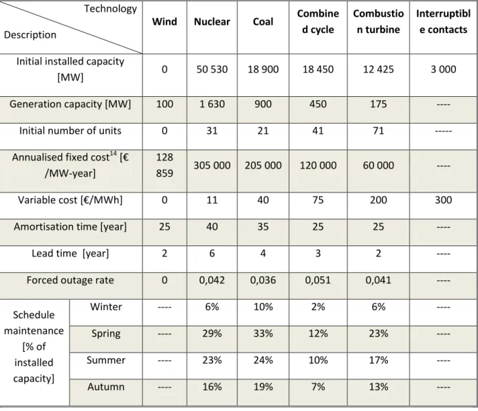
The model represents a market which holds wind power generation and thermal-generating units with four different technologies including nuclear (N), hard-coal (HC), combined cycle gas turbine (CCGT) and oil-fired combustion turbine (CT). These thermal technologies are characterised by outages and schedule maintenance. Interruptible contracts are seen as a generation technologies with variable cost and no fixed cost.
In the case of a subsidised wind development, we add exogenously constant capacity equal to 2000 MW (60,000 MW at the end of the simulation period) for each period τ (in years), which is assumed to correspond to the target set by the regulator and supported by a feed-in-tariff policy. The key figures for each plant type are shown in Table 1.
16
Table 1.Generation data used in simulations
Technology Description
Wind Nuclear Coal Combine
d cycle
Combustio n turbine
Interruptibl e contacts
Initial installed capacity
[MW] 0 50 530 18 900 18 450 12 425 3 000
Generation capacity [MW] 100 1 630 900 450 175 ----
Initial number of units 0 31 21 41 71 ---
Annualised fixed cost14 [€ /MW-year]
128
859 305 000 205 000 120 000 60 000 ----
Variable cost [€/MWh] 0 11 40 75 200 300
Amortisation time [year] 25 40 35 25 25 ----
Lead time [year] 2 6 4 3 2 ----
Forced outage rate 0 0,042 0,036 0,051 0,041 ----
Schedule maintenance [% of installed capacity] Winter ---- 6% 10% 2% 6% ---- Spring ---- 29% 33% 12% 23% ---- Summer ---- 23% 24% 10% 17% ---- Autumn ---- 16% 19% 7% 13% ----
Electricity demand is characterised by a load-duration curve, which illustrates a cumulative distribution of demand levels over each year during the simulation period, and is derived from data on the French electricity consumption in 2010.15We split the load-duration curve (
Fig.2) in 40 segments of extreme peak hours and 40 segments of 218 hours each one for the
remaining hours (peak, intermediate and off-peak hours). We also assume a Kendall’s coefficient equal to 0.3 which, as noted above, represents the level of concordance between wind power generation and demand. As previously mentioned, we consider two uncertain components affecting demand: its growth rate and thermo-sensitivity.16
14
The discount rate is set at 8%.
15
See http://clients.rte-france.com/lang/fr/visiteurs/vie/vie_stats_conso_inst.jsp
17
Fig.2. Load-duration curve
To calculate the electricity price, we assume perfect competition hence the price is generally settled by the marginal cost of generation i.e. the variable cost of the marginal technology. However, if demand exceeds the available generation capacity, the electricity price is equal to the cost of interruptible load contracts. Finally, the electricity price is set at the value of loss of load (with a VOLL set at 20 000 €/MWh), whether or not the volume of interruptible contracts is exhausted, or whether demand is curtailed. The adequacy target for the system is determined by the reliability index of LOLE which is set at 3 hours of shortage per year.
The resolution time-step of the model is one year, using the simplifying assumption that investment decisions can only be made at the beginning of each year. To test the level of uncertainty, 4000 random scenarios, of 30-year period each, are generated through a Monte Carlo simulation method. The model has been developed as a set of programs using Matlab.
4.2 Subsidised wind power development scenarios
In this subsection, we compare the effect of the subsidised development of wind power for an energy-only market with a price cap set at 3000 €/MWh (Case 1) and for a market with a forward capacity market and the same price cap (Case 2).The starting point is an optimised mix of generation technologies with no wind power. We use this optimal mix as a reference case, with which to compare the generation mix in future years, once wind power is introduced. In the scenario with subsidised development, the main purpose of the capacity mechanism is to provide additional value to the technologies that contribute towards the generation adequacy criterion, and to trigger investments in peak-load generation technologies.
18
4.2.1. Case1: Subsidised development of wind power in an energy-only market with price cap
Fig.3 illustrates the evolution of the generation mix in terms of installed capacity. Despite the exogenous introduction of wind power, installed capacity increases for all technologies as a result of demand growth. To isolate the effect of demand growth on the evolution of the generation mix, we illustrate the evolution of the thermal generation mix(independent of wind power development) in Fig.4. We note that after the introduction of wind power, the less capital-intensive technologies (CCGT and CT) increase their share in the thermal generation mix whilst the shares of base- and middle-load technologies (nuclear and coal) are reduced. Thus, the share of nuclear generation capacity in the thermal generation mix falls from 50% (48.9 GW) in year 1 to 44% (53.2 GW) in year 30. The share of coal generation capacity increases from 19% (18 GW) in year 1 to 16% (19.8 GW) in year 30. In terms of the share of less capital-intensive technologies, CCGT generation capacity increases from 19% (18 GW) in year 1 to 22% (26.1 GW) in year 30, and the CT generation capacity from 12% (12.1 GW) in year 1 to 18% (21.7 GW) in year 30.
Fig.3. Dynamics of generation mix in the energy-only market with subsidised wind power development – case 1
The dynamic evolution of the thermal generation mix over the simulation period shows that the high penetration of wind power leads to an increase in the share of flexible and low capital-intensive generation technologies such as CCGT and TC. This result seems counterintuitive: recall that in a market with a price cap, the “missing money” effect is disincentive to generation investments, and particularly high in peaking units which are capital intensive per generated MWh. However the pressure exerted by the need for generation capacity in capital-intensive peaking units resulting from wind power development, is more important than the disincentive effect induced by the price cap – that is, to invest in peak-load generation in response to the “missing money” problem. As we shall see later, although the share of flexible generation in the thermal generation mix increases, the impact of the price cap leads to a lack of generation capacity and security margin in the system to ensure generation adequacy.
19
Fig.4. Dynamics of shares in the thermal generation mix in the energy-only market with subsidised wind power development – case 1
Fig.5 and
Fig.6 display the results of the Monte Carlo simulation in terms of the security margin and installed
generation capacity. On the right Y-axis of Fig.5, we report the peak demand and installed generation capacity, and on the left Y-axis the security margin. The X-axis shows the years of simulation. As shown inFig.5, security margin increases significantly over the simulation period. Nevertheless, the installed generation capacity that results from this security margin development is not sufficient to guarantee the regulator’s adequacy target for the system (three hours of shortage per year), which indicates the low contribution of wind power generation to the long-term security of supply.
Indeed, an amplified price cycle would be necessary so that generation capacity investments can be triggered in due time and more frequently. The right Y-axis in
Fig.6 displays the annual average electricity price and the left Y-axis show the duration of power
shortages (averaged per year over all runs). It shows a strong relationship between the annual average electricity price and the duration of power shortages. For example, at the beginning of the simulation in year 1, there are three hours of shortage and an annual average electricity price equal to 46.1 €/MWh, whilst in year 3 there are 20.7 hours of shortage and an annual average electricity price equal to 53.7 €/MWh.
20
Fig.5. Installed generation capacity, peak-load and security margin in the energy-only market with subsidised wind power development – case 1
Both the wide variation in the duration of the shortage period, as well as the annual average electricity price in the first three years of the simulation, are explained by the optimal thermal generation mix set at the beginning of the simulation, which is determined by the regulated adequacy target. Since the hourly prices on the energy market are capped at 3000 €/MWh, three hours of shortage are insufficient to generate a revenue to cover development costs for new generation units. Consequently, generation capacity investments will be made if these prices reach the price cap level more frequently (around 20 hours per year in our simulation). This results in an amplification of the price cycle in the first three years of the simulation period. As we will see in the next case, when additional revenue from a capacity mechanism is added to the revenue from the energy market, the wide variations in the annual average electricity price associated with periods of tight capacity at the beginning of the simulation period disappears.
Fig.6. Hours of shortage and annual average electricity price in the energy-only market with subsidised wind power development – case 1
4.2.2. Case 2: Subsidised development of wind power in an energy-only market with price cap and capacity mechanism
21
Fig.7 shows the evolution of the mix of generation technologies in terms of installed capacity in the
case of a subsidised development of wind power in an energy-only market with price cap and capacity mechanism. As in the previous case, installed capacity increases for all generation technologies as a consequence of demand growth. However, this increase is more important than in case 1 because of the existence of the capacity mechanism that provides additional revenue for producers.
Fig.7. Dynamics of generation mix in the energy market with capacity mechanism and subsidised wind power development – case 2
With regards to the evolution of the thermal generation mix (
Fig.8), there is an increase in the share of the CT generation capacity, compared to case 1. It
increases from 12% (12.1 GW) in year 1 to 21% (25.8 GW) in year 30, compared to18% for the same year in case 1. The share of nuclear generation capacity declines significantly from 50% (48.9 GW) in year 1 to 41% (52.9 GW) in year 30, relative to44% in case 1. The share of CCGT generation capacity in contrast, remains roughly constant during the simulation period at around 19%, whilst it increases from 19%to 22% between years 1 and 30 in case 1.
22
Fig.8. Dynamics of shares in the thermal generation mix in the energy market with capacity mechanism and subsidised wind power development – case 2
Now turning to the issue of generation adequacy, evolutions of security margin, installed generation capacity and peak demand are presented in
Fig.9 as shown similarly for the previous cases. The security margin and the total installed capacity
increase to a greater extent compared to case 1. This suggests that the existence of additional capacity revenue for producers solves the “missing money” problem and leads to a higher security margin compared to case 1. The installed generation capacity is higher by 5.7 GW than in case 1 (186.4 GW instead of 180.7 GW) and this leads to improved reliability performances such that the adequacy target is met.
Fig.9. Installed generation capacity, peak-load and security margin in the energy market with capacity mechanism and subsidised wind power development – case 2
This security margin contributes to the fulfillment of the regulated adequacy target (3 hours of shortage per year) over the simulation period, as illustrated in
Fig.10. This suggests that the security constraint, which is implicitly introduced by the design of the
capacity mechanism, adds value to the contribution of each generation technology to the long-term security of supply. It therefore guarantees that the regulated adequacy target will not be exceeded.
23
Fig.10. Hours of shortage and annual average electricity price in the energy market with capacity mechanism and subsidised wind power development – case 2
With respect to the producers’ annual average income, we add the capacity revenue to the energy revenue in order to compare the “electricity revenue” indicator. The latter is obtained from the electricity price in the case of the energy-only market with price cap (case 1).
Fig.10 shows the results. It is worth noting that the wide variations observed in terms of price and security margin in the early years of the simulation period in case 1disappear in this case 2. Indeed, as investors have additional revenue from the capacity mechanism at the beginning of the simulation period, they do not need to wait for initial price spikes to invest in new generation capacity. At the same time, the annual average electricity price is lower relative to case 1 because there are fewer episodes of scarcity and consequently, energy prices spike during peak hours are less recurrent.
4.3. Effect of the market-driven development of wind power
In this subsection, we compare the effect of the market-driven development of wind power for a scenario with an energy-only market with a price cap set at 3000 €/MWh (Case 3), and a similar scenario but additionally with a forward capacity market (Case 4).
We consider a decline in the investment cost of wind generation, set at 1.5%/year, which reflects an exogenous learning effect. This learning effect allows wind power to cross the threshold of competitiveness from a certain date. In order to interpret the results of cases 3 and 4, it is noteworthy that the capacity mechanism has the dual function of giving an additional value to every generation technology (and more importantly to peak-load and flexible units) on one hand, and also giving a much lower value to wind power units on the other. The latter is due to their limited contribution to the system reliability and capacity adequacy.
24
Fig.11 illustrates the evolution of the generation mix. Once it turns competitive in year 6, wind power
starts to develop and reaches an installed capacity of 34.8 GW in year 30. This is significantly lower than the development target in the two previous cases of subsidised development (60 GW in year 30). With regard to the thermal generation technologies, capacity increases over the simulation period. The increase in nuclear generation capacity is greater than in the case with subsidised development of wind power (case 1 and case 2) whilst the level of CT generation capacity is similar to the previous cases. This is a consequence of a reduced requirement for additional reserve margins (and system flexibility) due to a lower wind power development. Furthermore, relative to cases 1 and 2, the decline in wind power penetration leads to a significant increase in the nuclear generation capacity over the simulation period.
Fig.11. Dynamics of generation mix in the energy-only market with market-driven wind power development – case 3
In
Fig.12, the evolution of the thermal generation mix is described by the concave shape of the curves
with an inflection point in year 15. The evolutions are not the same before and after this point in time. During the first fifteen years, the share of flexible generation capacity in the thermal generation mix decreases whilst base-load generation capacity increases. The share of the CT generation capacity decreases from 12% (12.1 GW) in year 1 to 10% (11.2 GW) in year 15.The share of nuclear generation capacity increases from 50% (48.9 GW) in year 1 to 54% (57.9 GW) in year 15. As for coal, the share in the thermal generation technology mix decreases from 19% (18 GW) in year 1 to 17% (18.1 GW) in year 15. In contrast, the share of CCGT remains constant at around 19% for the same period. These results confirm the disincentive effect of establishing a price cap on investments in peak-load generation technologies. Unlike case 1, here, the weaker share of wind power (relative to case 1) results in a low need for an additional security margin during the first years, thus preventing the onset of significant investments in peak-load generation units.
25
Fig.12. Dynamics of shares in the thermal generation mix in the energy-only market with market-driven wind power development – case 3
As shown in
Fig.12, although initial wind power development occurs from year 5, it is only after year 15 that the need for additional security margin increases sufficiently such that investments in flexible generation become profitable. For example, the share of the CT generation capacity increases from 10% (11.2 GW) in year 15 to 13% (16.3 GW) in year 30 whilst the share of nuclear generation capacity decreases from 54% (57.9 GW) in year 15 to 49% (60.6 GW) in year 30.
Fig.13. Installed generation capacity, peak-load and security margin in the energy-only market with market-driven wind power development – case 3
Fig.13 illustrates the generation adequacy indicators in case 3. The security margin increases over the
simulation period, in particular after year 15 when wind power capacity develops more significantly. This variation is also reflected in the hours of shortage, as shown in
26
Fig.14. As in case 1, after the first four years, the number of hours of shortage is higher than the
regulated adequacy target (3 hours of shortage per year). As was mentioned earlier, these variations are related to the need to amplify the price cycles and provide large scarcity rents, in order to trigger investment in new generation capacity (in particular in peaking units). Market-driven wind power development is therefore at the expense of reliability performances when electricity prices are capped.
Fig.14. Hours of shortage and annual average electricity price in the energy-only market with market-driven wind power development – case 3
Here, the annual average electricity price is lower compared to case 1. This results from the fact that the development of the CT generation capacity is lower than in case 1 as a consequence of the low development of wind power. The results show that, where wind power development is driven by the market and not exogenously imposed, the intuition that ambitious promotion policy for wind power results in a substantial fall in electricity price, does not hold.
4.3.2. Case 4: Market-driven development of wind power in an energy-only market with a price cap and capacity mechanism
Fig.15 illustrates the evolution of the generation capacity mix, in the case of
market-driven development of wind power in an energy-only market with a price cap (3000 €/MWh) and capacity mechanism. As expected, the results show that wind power capacity develops later and more slowly compared to the previous cases, since the capacity mechanism gives an additional value to generation units that provide firm energy during scarcity periods. Investments in wind power generation start to develop in year 9 – later than in the previous case (year 6). The installed wind power capacity reached in year 30 is lower than in case 3 (26.8 GW compared to34.8 GW). This results from the security constraint of firm energy which is implicit to the implementation of a capacity mechanism. It penalises wind power development compared to firm conventional generation capacity because of its low contribution to the system generation adequacy.
27
Fig.15. Dynamics of generation mix in the energy market with capacity mechanism and market-driven wind power development – case 4
The evolution of the thermal generation mix is illustrated in
Fig.16. There is a slightly higher increase in the share of peak-load generation technologies in case 4
compared to case 3.This is due to the response to the low development of wind power, and a slight decrease in the base-load generation capacity. Specifically, the share of CT in the thermal generation capacity mix increases by 4% (from 12.1 GW in year 1 to 19.7 GW in year 30) over the simulation period instead of 3%, in case 3. The share of nuclear generation capacity declines from 50% (48.9 GW) in year 1 to 48% (62.4 GW) in year 30, instead of 1% in the previous case.
Fig.16. Dynamics of shares in the thermal generation mix in the energy market with capacity mechanism and market-driven wind power development – case 4
28
Fig.17 shows the results for the generation adequacy indicators. The evolution of the generation
capacity is slightly higher than in case 3 for the first fifteen years, whilst it is slightly lower than in case 3 for the rest of the simulation period. The security margin is higher than in case 3 during the first 15 years (pushed up by the incentive effect of the capacity mechanism on generation capacity investment), but beyond year 15, wind power development becomes significantly lower in case 4 than in case 3.This results from the reduced need for additional capacity margins. Therefore, there is a lower increase in peak-load generation capacity investments in case 4 compared to case 3. Yet this is not sufficient to ensure generation adequacy in case 3, whilst regulated adequacy target is reached in case 4 under the security constraint imposed by the design of the capacity mechanism, as previously mentioned.
Fig.17. Installed generation capacity, peak-load and security margin in the energy market with capacity mechanism and market-driven wind power development – case 4
Fig.18 shows the evolution of the reliability index of LOLE in case 4. The number of shortage hours
remains approximately at the level of the adequacy target over the simulation period. Furthermore, by comparing results concerning the evolution of the annual average electricity price (energy price plus capacity revenue) between case 2 and case 4, the two cases with a capacity mechanism, there is a lower average electricity price when a market-driven development approach is adopted. This is because wind power in case 4 is less developed than in case 2, which, in turn, results in a smaller share of peaking units needed in the thermal generation mix in order to reach the adequacy target.
29
Fig.18. Hours of shortage and annual average electricity price in the energy market with a capacity mechanism and subsidised wind power development – case 4
4.4. Performance comparison in terms of price volatility and social costs of different types of
development for wind power
In this section, we compare the performance indicators in terms of price and cost of each type of development for wind power with or without the use of a capacity mechanism to compensate for long-term negative externalities. To do so, we first examine the impact of increasing penetration of wind power on the annual spot price distribution. We then compare the social costs associated with each type of wind power scenario with and without a capacity mechanism.
4.4.1. Effects of different types of wind power development upon the short-term prices distribution
Fig.19 and
Fig.20 display the price duration curves17for the two types of wind power development scenarios. In
each figure, the dotted curve represents the price duration curve at the beginning of the simulation in year 0 in which there is no wind power. The solid curve represents the price duration curve in year 30 for case 1 and 3 respectively, while that the dashed curve represents the price duration curve in year 30 for case 2 and 4 respectively.
30
Fig.19. Energy prices-duration curve in subsidized development cases
In the two wind power development scenarios, beyond the relative similarity of the three curves in
Fig.19 and
Fig.20, we find that the introduction of large-scale wind power generation leads to a reduction of
hours in which the price is set by base- and middle-load generation units. Therefore, the price rise to the marginal costs of peak-load generation units for several more hours. Another consequence is the downward movement of prices, which is attributed to the shifts in the merit order curve to the right when the penetration of wind power increases. However, this effect is partly compensated by the reduction of base-load generation capacity at the end of the simulation period and by its substitution of the with peak-load generation technologies which are more flexible but has higher marginal costs. When comparing the price duration curve in year 30 in case 1 (energy-only market with price cap) and that in case 2 (energy market with capacity mechanism), we find that prices are higher in the first case and mainly during peak- and middle-load hours. This is because in case 1, the price cap policy without a capacity mechanism leads to a reduction in generation capacity investment, in particular in peak-load generation technologies. Therefore, hourly prices in case 1 are set more frequently at the marginal cost of base- and middle-load generation units compared to case 2, in which there is a capacity mechanism that gives an additional incentive to invest in peak-load generation units.
31
Fig.20. Energy price-duration curve in market-driven development cases
In scenarios with market-driven development of wind, differences between price duration curves for case 3 and case 4 shown in
Fig.20 are lower than those observed with subsidised development. This can be explained by the fact
that in cases of market-driven development, wind power capacity is significantly lower than in cases of subsidised development (34.8 GW and 26.8 GW for cases 3 and 4 compared to 60 GW in cases 1 and 2).This implies smaller impacts in terms of price volatility following the introduction of wind power, as well as smaller dynamic impacts on the thermal generation mix.
4.4.2. The cost of the different types of wind power development with and without capacity mechanism
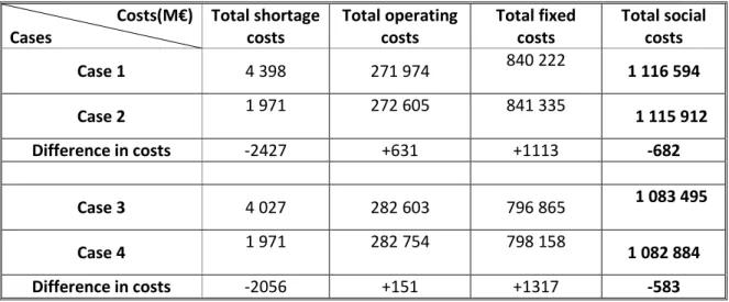
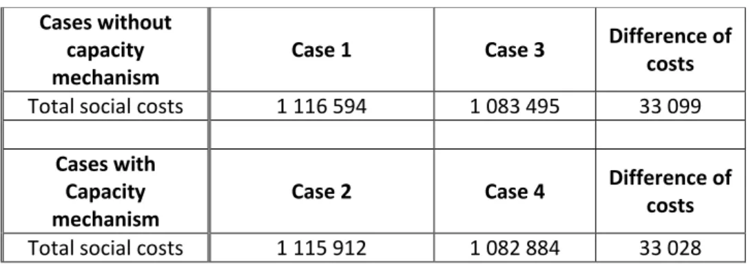
Given that the generation mix can change significantly if large amounts of wind power are introduced in the system, we can compare what the cost impacts associated with the change in the portfolio mix. In this subsection, we address this question by comparing the total cost over the simulation period for the four cases previously studied. The total social cost is calculated as the sum of three different components: the capital expenditures (fixed costs), the operating costs and the shortage cost.
Calculating and comparing total costs requires additional assumptions, in the cases of subsidised wind power development. As mentioned in section 3, the investment costs in wind power capacity in cases 1 and 2 are determined exogenously in our model. Therefore, for the sake of the comparison, we assume that the investment costs in wind power capacity in case 1 and case 2 are similar to those in the case of market-driven development cases. This assumption implies a reduction in the feed-in-tariff set by the regulator, to take into account the investment costs reduction achievable by the learning effect. Although at first glance this assumption seems to question the relevance of subsidizing the development for wind power (as the regulator could let the energy market develop wind power at its own pace), our results show that a market-driven development is not sufficient to