Hyperparameter optimization with approximate gradient

(1)

Fabian Pedregosa F@BIANP.NET

Chaire Havas-Dauphine “ ´Economie des Nouvelles Donn´ees”

CEREMADE, CNRS UMR 7534, Université Paris-Dauphine, PSL Research University Département Informatique de l’ École Normale Supérieure, Paris

Abstract

Most models in machine learning contain at least one hyperparameter to control for model com-plexity. Choosing an appropriate set of hyper-parameters is both crucial in terms of model ac-curacy and computationally challenging. In this work we propose an algorithm for the optimiza-tion of continuous hyperparameters using inex-act gradient information. An advantage of this method is that hyperparameters can be updated before model parameters have fully converged. We also give sufﬁcient conditions for the global convergence of this method, based on regularity conditions of the involved functions and summa-bility of errors. Finally, we validate the empirical performance of this method on the estimation of regularization constants of �2-regularized

logis-tic regression and kernel Ridge regression. Em-pirical benchmarks indicate that our approach is highly competitive with respect to state of the art methods.

1. Introduction

Most models in machine learning feature at least one hy-perparameter to control for model complexity. Regular-ized models, for example, control the trade-off between a data ﬁdelity term and a regularization term through one or several hyperparameters. Among its most well-known instances are the LASSO (Tibshirani, 1996), in which �1

regularization is added to a squared loss to encourage spar-sity in the solutions, or �2-regularized logistic regression, in

which squared �2regularization (known as weight decay in

the context of neural networks) is added to obtain solutions with small euclidean norm. Another class of

hyperparam-Proceedings of the 33rd _{International Conference on Machine}

10−2 ₁₀−1 ₁₀0 ₁₀1 ₁₀2 ₁₀3 ₁₀4 ₁₀5 regularization parameter cross-vali dat ion loss

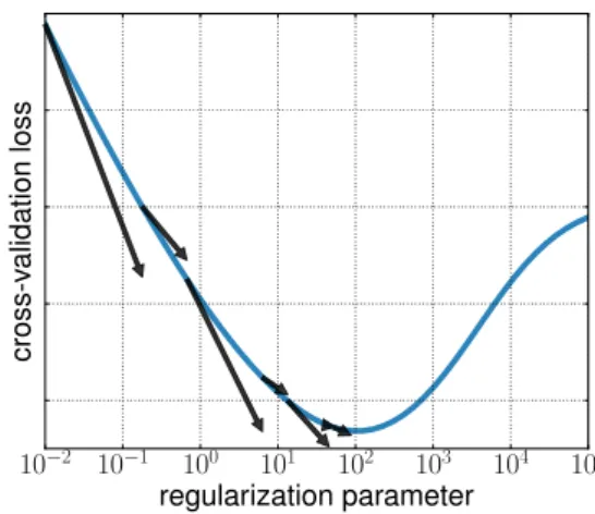
Figure 1. Hyperparameter Optimization with approximate gradi-ent. The gradient of the cross-validation loss function with re-spect to hyperparameters is computed approximately. This noisy gradient is then used to estimate the optimal hyperparameters by gradient descent. A decreasing bound between the true gradient and the approximate gradient ensures that the method converges towards a stationary point.

eters are the kernel parameters in support vector machines. For example, the popular radial basis function (RBF) nel depends on a “width” parameter, while polynomial ker-nels depend on a discrete hyperparameter specifying the degree. Hyperparameters can be broadly categorized into two groups: continuous hyperparameters, such as regular-ization parameters or the width of an RBF kernel and dis-crete hyperparameters, such as the degree of a polynomial. In this work we focus on continuous hyperparameters. The problem of identifying the optimal set of hyperparam-eters is known as hyperparameter optimization. Hyperpa-rameters cannot be estimated to minimize the same cost function as model parameters, since this would favor mod-els with excessive complexity. For example, if regulariza-tion parameters were chosen to minimize the same loss as model parameters, then models with no regularization would always yield the smallest loss. For this reason, hy-perparameter optimization algorithms seek to optimize a criterion of model quality which is different from the cost

(2)

function used to ﬁt model parameters. This criterion can be a goodness of ﬁt on unseen data, such as a cross-validation loss, or some criteria of model quality on the train set such as SURE (Stein, 1981), AIC/BIC (Liu and Yang, 2011) or Mallows Cp(Mallows, 1973), to name a few.

Choosing the appropriate set of hyperparameters has often a dramatic inﬂuence in model accuracy and many hyperpa-rameter optimization algorithms have been proposed in the literature. For example, in the widely used grid-search al-gorithm, the model is trained over a range of values for the hyperparameters and the value that gives the best perfor-mance on the cross-validation loss is chosen. This not only scales poorly with the number of hyperparameters, but also involves ﬁtting the full model for values of hyperparame-ters that are very unpromising. Random search (Bergstra et al., 2011) has been proven to yield a faster exploration of the hyperparameter space than grid search, specially in spaces with multiple hyperparameters. However, none of these methods make use of previous evaluations to make an informed decision of the next iterate. As such, conver-gence to a global minima can be very slow.

In recent years, sequential model-based optimization (SMBO) techniques have emerged as a powerful tool for hyperparameter optimization (see e.g. (Brochu et al., 2010) for an review on current methodologies). These techniques proceed by ﬁtting a probabilistic model to the data and then using this model as an inexpensive proxy in order to deter-mine the most promising location to evaluate next. This probabilistic model typically relies on a Gaussian process regressor but other approaches exist using trees (Bergstra et al., 2011) or ensemble methods (Lacoste et al., 2014). The model is built using only function evaluations, and for this reason SMBO is often considered as a black-box opti-mization method.

A third family of methods, which includes the method that we present, estimate the optimal hyperparameters using smooth optimization techniques such as gradient descent. We will refer to these methods as gradient-based hyper-parameter optimization methods. These methods use local information about the cost function in order to compute the gradient of the cost function with respect to hyperparame-ters. However, computing the gradient with respect to hy-perparameters has reveled to be a major bottleneck in this approach. For this reason we propose an algorithm that re-places the gradient with an approximation. More precisely, we make the following contributions:

• We propose a gradient-based hyperparameter opti-mization algorithm that uses approximate gradient in-formation rather than the true gradient.

• We provide sufﬁcient conditions for the convergence of this method to a stationary point.

• We compare this approach against state-of-the art methods for the task of estimation of regularization and kernel parameter on two different models and three datasets.

Notation We denote the gradient of a real-valued function by ∇. If this function has several input arguments, we de-note ∇iits gradient with respect to the i-th argument.

Sim-ilarly, ∇2 _{denotes the Hessian and ∇}2

i,j denotes the

sec-ond order differential with respect to variables i and j. For functions that are not real-valued, we denote its differential by D. We denote the projection operator onto a set D by PD. That is, PD(α)� arg minλ∈D�α − λ�2, where � · �

denotes the euclidean norm for vectors.

Throughout the paper we take the convention of denot-ing real-valued functions with lowercase letters (such as f and g) and vector-valued functions with uppercase let-ters (such as X). Model paramelet-ters are denoted using low-ercase Latin letters (such as x) while hyperparameters are denoted using Greek lowercase letters (such as λ).

1.1. Problem setting

As mentioned in the introduction, the goal of hyperparam-eter optimization is to choose the hyperparamhyperparam-eters λ that optimizes some criteria, such as a cross-validation loss or a SURE/AIC/BIC criteria. We will denote this criteria by f : Rs → R, where s is the number of hyperparameters. In its simplest form, the hyperparameter optimization prob-lem can be seen as the probprob-lem of minimizing the cost func-tion f over a domain D ⊆ Rs_{. Some approaches, such as}

sequential model-based optimization, only require function evaluations of this cost function. The methods we are in-terested in however use local information of the objective function.

The cost function f (e.g. the cross-validation error) de-pends on the model parameters, which we will denote by X(λ). These are commonly not available in closed form but rather deﬁned implicitly as the minimizers of some cost function that we will denote h(·, λ) : Rp_{→ R, where p is}

the number of model parameters. This makes the hyperpar-mater optimization problem can be naturally expressed as a nested or bi-level optimization problem:

arg min λ∈D � f (λ)� g(X(λ), λ)� s.t. X(λ) ∈ arg min x∈Rp h(x, λ) , (HO) where the minimization over h is commonly referred to as the inner optimization problem. A notable example of hyperparameter optimization problem is that of regulariza-tion parameter selecregulariza-tion by cross-validaregulariza-tion. For

(3)

simplic-ity, we restrict the discussion to the case of simple or hold-out cross-validation, where the dataset is split only once, although the methods presented here extend naturally to other cross-validation schemes. In this setting, the dataset is split in two: a train set (denoted Strain) and a test or

hold-out set (denoted Stest). In this case, the outer cost function

is a goodness of ﬁt or loss on the test set, while the inner one is a trade-off between a data ﬁtting term on the train set and a penalty term. If the penalty term is a squared �2-norm, then the problem adopts the form:

arg min λ∈D loss(Stest, X(λ)) s.t. X(λ) ∈ arg min x∈Rp loss(Strain, x) + e λ �x�2 _. (1)

The trade-off in the inner optimization between the good-ness of ﬁt term and the penalty term is controlled through the hyperparamter λ. Higher values of λ bias the model pa-rameters towards vectors with small euclidean norm, and the goal of the hyperparameter optimization problem is to ﬁnd the right trade-off between these two terms. The parametrization of the regularization parameter by an ex-ponential (eλ_{) in Eq. (1) might seem unusual, but given that}

this regularization parameter is commonly optimized over a log-spaced grid, we will ﬁnd this parametrization useful in later sections.

Turning back to the general problem (HO), we will now describe an approach to compute the derivative of the cost function f with respect to hyperparameters. This approach, which we will refer to as implicit differentiation (Larsen et al., 1996; Bengio, 2000; Foo et al., 2008), relies on the observation that under some regularity conditions it is pos-sible to replace the inner optimization problem by an im-plicit equation. For example, if h is smooth and veriﬁes that all stationary points are global minima (as is the case for convex functions), then the values X(λ) are character-ized by the implicit equation ∇1h(X(λ), λ) = 0. Deriving

the implicit equation with respect to λ leads to the equation ∇2

1,2h +∇21h· DX = 0, which, assuming ∇21hinvertible,

characterizes the derivative of X. The chain rule, together with this equation, allows us to write the following formula for the gradient of f:

∇f = ∇2g + (DX)T∇1g =∇2g− � ∇2 1,2h �T� ∇2 1h �−1 ∇1g . (2) This formula allows to compute the gradient of f given the following quantities: model parameters X(λ) (g and h are evaluated at (X(λ), λ)) and �∇2

1h

�−1

∇1g, which

is usually computed as the solution to the linear system �

∇2 1h

�

z = ∇1g for z. In the section that follows, we

present an algorithm that relaxes the condition of both knowledge of the exact model parameters and exact solu-tion of the linear system.

2. H

OAG

: Hyperparameter

optimiza-tion with approximate gradient

As we have seen in the previous section, computing an ex-act gradient of f can be computationally demanding. In this section we present an algorithm that uses an approx-imation, rather than the true gradient, in order to estimate the optimal hyperparameters. This approach yields a trade-off between speed and accuracy: a loose approximation can be computed faster but might result in slow convergence or even divergence of the algorithm. At iteration k, this trade-off is balanced by the tolerance parameter εk. The

sequence of tolerance parameters {ε1, ε2, . . .} will turn out

to play a major role in the convergence of the algorithm, al-though the time being, we will treat it as free parameter. We now describe our main contribution, the HOAGalgorithm:

Algorithm 1 (HOAG). At iteration k = 1, 2, . . .

per-form the following:

(i) Solve the inner optimization problem up to tol-erance εk. That is, ﬁnd xksuch that

�

�X(λk)− xk�� ≤ εk .

(ii) Solve the linear system ∇2

1h(xk, λk)qk =

∇1g(xk, λk)for qk up to tolerance εk. That is,

ﬁnd qksuch that � � �∇21h(xk, λk)qk− ∇1g(xk, λk) � � � ≤ εk .

(iii) Compute approximate gradient pkas

pk =∇2g(xk, λk)− ∇21,2h(xk, λk)Tqk ,

(iv) Update hyperparameters: λk+1= PD � λk− 1 Lpk � .

This algorithm consists of four steps. The ﬁrst two steps of the algorithm compute approximations to the quantities used in Eq. (2) to compute the gradient of f. However, since these are not computed to full accuracy, pk, computed

in step (iii) is a noisy estimate of the gradient. This approx-imation is then used as a replacement of the true gradient in a projected gradient-descent (iv) iteration.

This procedure requires access to three quantities at itera-tion k: a εk-optimal solution to the inner optimization

prob-lem which can be computed with any solver, the ﬁrst-order derivatives of g, (∇1g,∇2g), and an εk-optimal solution

to a linear system involving ∇2

(4)

is solved using a conjugate-gradient method, which only requires access to the matrix ∇2

1h through matrix-vector

products. For example, in machine learning problems such as the ones introduced in Eq. (1), the quantity ∇2

1h

cor-responds to the Hessian of the inner optimization prob-lem. Efﬁcient schemes for multiplication by the Hessian can be derived for least squares, logistic regression (Lin et al., 2008) and other general loss functions (Pearlmutter, 1994).

2.1. Related work

There exists a large variety of hyperparameter optimization methods, and a full review of this literature would be out-side the scope of this work. Below, we comment on the relationship between HOAGand some of the most closely

related methods.

Regarding gradient-based hyperparameter optimization methods we will distinguish two main approaches, implicit differentiation and iterative differentiation, depending on how the gradient with respect to hyperparameters is com-puted.

Implicit differentiation. This approach consists in deriv-ing an implicit equation for the gradient usderiv-ing the optimal-ity conditions of the inner optimization problem (as we did in Eq. (2)). Originally motivated by the problem of set-ting the regularization parameter in the context of neural networks (Larsen et al., 1996; 1998; Bengio, 2000), has also been applied to the problem of selecting kernel pa-rameters (Chapelle et al., 2002; Seeger, 2008) or multiple regularization parameters in log-linear models (Foo et al., 2008). This approach has also been successfully applied to the problem of image reconstruction (Kunisch and Pock, 2013; Calatroni et al., 2015), in which case the simplicity of the cost function function allows for a particularly simple expression of the gradient with respect to hyperparameters. Iterative differentiation. In this approach, the gradient with respect to hyperparameters is computed by differen-tiating each step of the inner optimization algorithm and then using the chain rule to aggregate the results. Since the gradient is computed after a ﬁnite number of steps of the inner optimization routine, the estimated gradient is natu-rally an approximation to the true gradient. This method was ﬁrst proposed by Domke (2012) and later extended to the setting of stochastic gradient descent by Maclaurin et al. (2015). We note also that contrary to the implicit differen-tiation approach, this method can be applied to problems with non-smooth cost functions (Deledalle et al., 2014; Ochs et al.).

HOAG, while belonging to the class of implicit

differentia-tion methods, is related to iterative differentiadifferentia-tion methods

in that it allows the gradient with respect to hyperparame-ters to be computed approximately.

Finally, we note that similar approaches have also been considered in the setting ofsequential model-based op-timization. Swersky et al. (2014) proposes an approach in which the inner optimization is “freezed” whenever the method decides that the current hyperparameter values are not promising. It does so by introducing a prior on train-ing curves as a function of input hyperparameters. This ap-proach however requires to make strong assumptions on the shape of the training curves which gradient-based methods do not make.

3. Analysis

In this section we will prove that the summability of the tolerance sequence {εi}∞i=1 is sufﬁcient to guarantee

con-vergence of the iterates in HOAG. The analysis of this al-gorithm is inspired by the work of d’Aspremont (2008); Schmidt et al. (2011); Friedlander and Schmidt (2012) on inexact-gradient algorithms for convex optimization. We will start this section by enumerating the regularity con-ditions that we assume for the hyperparameter optimization problem. The following conditions are assumed through the section:

• (A1) L-smoothness. We assume that the ﬁrst deriva-tives of g and the second derivaderiva-tives of h are Lipschitz continuous functions.

• (A2) Nonsingular Hessian. We assume that the ma-trix ∇2

1h, which corresponds to the Hessian of the

in-ner optimization problem, is invertible at the values (X(λ), λ), λ_{∈ D.}

• (A3) Convex compact domain. The domain under which the hyperparameters are optimized, D, is a con-vex non-empty and compact subset of Rs_.

These assumptions are veriﬁed by many models of inter-est. For example, for the problem of estimation of regular-ization parameters of Eq. (1), it allows twice-differentiable loss functions such as logistic regression or least squares (assumption A1) and strongly convex penalties (A2), such as squared �2 regularization. Note that condition (A2)

need not be veriﬁed on all its domain, only on the points (X(λ), λ), which would allow in principle to consider models that are deﬁned through a non-convex cost func-tions. Assumption (A3) requires that the domain of the hy-perparameters is a convex compact domain. In practice, hyperparameters are optimized over a s-dimensional inter-val, i.e., a domain of the form D = [a1, b1]× · · · [as, bs].

(5)

Our analysis however only require this domain to be con-vex and compact, a constraint that subsumes s-dimensional intervals.

The rest of the section is devoted to prove (under condi-tions) the convergence of HOAG. The proof is divided in

two parts. First, we will prove that the difference between the true gradient and the approximate gradient is bounded by O(ε) (Theorem 1) and in a second part we will prove that if the sequence {εi}∞i=1is summable, then this implies

the convergence to a stationary point of f (Theorem 2). Be-cause of space limitation, the proofs are omitted and can be found in Appendix A.

Theorem 1 (The gradient error is bounded). For sufﬁ-ciently large k, the error in the gradient is bounded by a constant factor of εk. That is,

�

�∇f(λk)− pk

�

� = O(εk) .

This theorem gives a bound on the gradient from the se-quence that bounds the inner optimization and the linear system solution. Is will be the key ingredient in order to show convergence to a stationary point, which is the main result of this section. This property sometimes referred to as global convergence (Nocedal and Wright, 2006): Theorem 2 (Global convergence). If the tolerance se-quence is summable, that is, if {ε}n

i=1is positive and

veri-ﬁes

∞

�

i=1

εi<∞ ,

then the sequence λkof iterates in the HOAGalgorithm has

limit λ∗ _{∈ D, and this limit veriﬁes the stationary point}

condition:

�∇f(λ∗), α_{− λ}∗_{� ≥ 0 , ∀α ∈ D .}

In particular, if λ∗_{belongs to the interior of D it is veriﬁed}

that

∇f(λ∗) = 0 .

This results gives sufﬁcient conditions for the convergence of HOAG. The summability of the tolerance sequence

sug-gest several natural candidates for this sequence, such as the quadratic sequence, εk = k−2 or the exponential

se-quence, εk = ρk, with 0 < ρ < 1. We will empirically

evaluate different tolerance sequences on different prob-lems and different datasets in the next section.

Experiments

In this section we compare the empirical performance of HOAG. We start by discussing some implementation

de-tails such as the choice of step size. Then, we compare

the convergence of different tolerance decrease strategies that were suggested by the theoretical analysis. In a third part, we compare the performance of HOAG against other hyperparameter optimization methods.

Adaptive step size. Our algorithm relies on the knowledge of the Lipschitz constant L for the cost function f. How-ever, in practice this is not known in advance. Furthermore, since the cost function is costly to evaluate, it is not feasi-ble to perform backtracking line search. To overcome this we use a procedure in which the step size is corrected de-pending on the gain estimated from the previous step. In the experiments we use this technique although we do not have a formal analysis of the algorithm for this choice of step size.

Let Δk denote the distance between the current iterate and

the past iterate, Δk =�λk− λk−1�. The L-smooth

prop-erty of the function g, together with Lemma 1, implies that there exists a constant M > 0 such that the following in-equality is veriﬁed:

g(λk, xk)≤ g(λk−1, xk−1) + Cεk+

εk−1(C + M )Δk− LΔ2k ,

(3) where C is the Lipschitz constant of g (for loss functions such as logistic or least squares this can easily be computed from the data). This inequality can be derived from the properties of L-smooth functions, and the details can be found in Appendix B. The procedure consists in decreasing the step (multiplication by α < 1) whenever the equation is not satisﬁed and to increase it (multiplication by β > 1) whenever the equation is satisﬁed to ensure that we are using a step size as large as possible. The constants that we used in the experiments are M = 1, α = 0.5, β = 1.05. Stopping criterion. The stopping criterion given in Al-gorithm 1 depends on X(λ) which is generally unknown. However, for objective functions in the inner optimiza-tion which are µ-strongly convex (µ/2 can be taken as the amount of regularization in �2-regularized objectives),

it is possible to lower bound the quantity �X(λk)− xk�

by µ−1_�g�_(λ

k, xk)�. Hence, it is sufﬁcient to ensure

µ−1_�g�_(λ

k, xk)� ≤ ε. Details can be found in Appendix B.

Initialization. The previous sections tells us how to adjust the step size but relies on an initial value of this parameter. We have found that a reasonable initialization is to initalize it to L = �p1� so that the ﬁrst update in HOAGis of

mag-nitude at most 1 (it can be smaller due to the projection), where p1is the approximate gradient on the ﬁrst step. The

initialization of the tolerance decrease sequence is set to ε1 = 0.1. We also limit the maximum precision to avoid

numerical instabilities to 10−12_{, which is also the precision}

for “exact” methods, i.e., those that do not use a tolerance sequence. The initialization of regularization parameters is set to 0 and the width of an RBF kernel is initialized to

(6)

− log(n feat), where n feat is the number of features or di-mensionality of the dataset.

Although HOAGcan be applied more generally, in our ex-periments we focus on two problems: �2-regularized

logis-tic regression and kernel Ridge regression. We follow the setting described in Eq. (1), in which an initial dataset is partitioned into two sets, a train set Strain = {(bi, ai)}ni=1

and a test set Stest = {(b�i, a�i)}mi=1, where ai denotes the

input features and bithe target variables.

The ﬁrst problem consists in estimating the regularization parameter in the widely-used �2-regularized logistic

regres-sion model. In this case, the loss function of the inner op-timization problem is the regularized logistic loss function. In the setting of classiﬁcation, the validation loss or outer cost function is commonly the zero-one loss. However, this loss is non-smooth and so does not verify assumption (A1). To overcome this and following (Foo et al., 2008), we use the logistic loss as the validation loss. This yield a problem of the form: arg min λ∈D m � i=1 ψ(b�ia�Ti X(λ)) s.t. X(λ) ∈ arg min x∈Rp n � i=1 ψ(biaTix) + eλ�x�2 , (4)

where ψ is the logistic loss, i.e., ψ(t) = log(1 + e−t_{). The}

second problem that we consider is that of kernel Ridge re-gression with an RBF kernel. In this setting, the problem contains two hyperparameters: the ﬁrst hyperparameter (λ1) controls the width of the RBK kernel and the second

hyperparameter (λ2) controls the amount of regularization.

The inner optimization depends on the kernel through the kernel matrix, formed by computing the kernel of all pair-wise input samples. We denote such matrix as K(γ)train,

where the (i, j) entry is given by k(ai, aj, γ), where k is the

RBF kernel function: k(ai, aj, γ) = exp(−γ�ai− aj�).

Similarly, the outer optimization also depends on the ker-nel through the matrix K(γ)test, where its entries are the

kernel product between features from the train set and fea-tures from the test set, that is, k(ai, a�j, γ). Denoting the

full hyperparameter vector as λ = [λ1, λ2], the kernel

ma-trix on the train set as, the full hyperparameter optimization problem takes the form

arg min λ∈D � � �b − Ktest(eλ1)X(λ) � � �2 s.t. �Ktrain(eλ1) + eλ2I � X(λ) = b , (5) where for simplicity the inner optimization is already set as an implicit equation. Note that in this setting, and unlike in the logistic regression problem, the outer optimization function depends on the hyperparameters not only through

the model parameters X(λ) but also through the kernel ma-trix.

The solver used for the inner optimization problem of the logistic regression problem is L-BFGS (Liu and Nocedal, 1989), while for Ridge regression we used a linear conju-gate descent method. In all cases, the domain for hyperpa-rameters is the s-dimensional interval [−12, 12]s_.

For the experiments, we use four different datasets. The dataset 20news and real-sim are studied with an �2

-regularized logistic regression model (1 hyperparameter) while the Parkinson dataset using a Kernel ridge regression model (2 hyperparameters). The MNIST dataset is investi-gated in a high-dimensional hyperparameter space using a similar setting to (Maclaurin et al., 2015, §3.2) and reported in in Appendix B. Datasets and models are described in more detail in Appendix B.

In all cases, the dataset is randomly split in three equally sized parts: a train set, test set and a third validation set that we will use to measure the generalization performance of the different approaches.

3.1. Tolerance decrease sequence

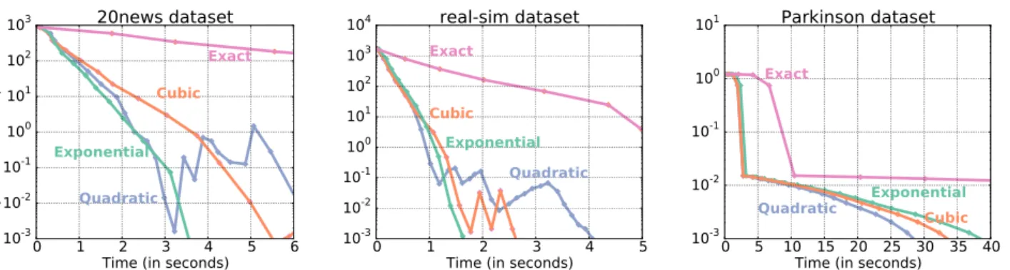
We report in Figure 2 the convergence of different tolerance decrease strategies. From Theorem 2, the sole condition on these sequences is that they are summable. Three no-table examples of summable sequences are the quadratic, cubic and exponential sequences. Hence, we choose one representative of each of these strategies. More precisely, the decrease sequences that we choose are a quadratic de-crease sequence of the form εk = 0.1× k−2, a cubic one

of the form εk = 0.1× k−3 and an exponential of the

form εk = 0.1× (0.9k). The value taken as true minima

of the hyperparameter optimization problem is computed by taken the minimum reached by 10 randomly initialized instances of HOAGwith exponential decrease tolerance. The plot shows the relative accuracy of the different vari-ants as a function of time. It can be seen that non-exact methods feature a cheaper iteration cost, yielding a faster convergence overall. Note that despite the global conver-gence result of Theorem 2, HOAG is not guaranteed to

be monotonically decreasing, and in fact, some degree of oscillation is expected when the decrease in the tolerance does not match the convergence rate (see e.g. Schmidt et al. (2011)). This can be appreciated in Figure 2, where the quadratic decrease sequence (and to some extent the cubit too) exhibits oscillations in the two ﬁrst plots.

(7)

� � � � � � � �� _{��} ��

Figure 2.Tolerance decrease strategies. Suboptimality as a function of time for different tolerance decrease strategies. The decrease sequences considered are quadratic (0.1k−2_{), cubic (0.1k}−3_{), exponential (0.1 × 0.9}k_{) and exact (gradient is computed to full accuracy}

at every iteration). Non-exact methods exhibit smaller cost per iteration, which results in faster convergence.

3.2. Comparison with other hyperparameter

optimization methods

We now compare against other hyperparameter optimiza-tion methods. The methods against which we compare are: • HOAG. The method we present in this paper, with an exponentially decreasing tolerance sequence. A Python implementation is made freely available at

https://github.com/fabianp/hoag.

• Grid Search. This method consists simply in split-ting the domain of the hyperparameter into an equally-spaced grid. We split the interval [−12, 12] into a grid of 10 values.

• Random. This is the random search method (Bergstra and Bengio, 2012) samples the hyperparameters from a predeﬁned distribution. We choose to samples from a uniform distribution in the interval [−12, 12]. • SMBO. Sequential model-based optimization

using Gaussian Process. We used the im-plementation found in the Python package BayesianOptimization (http://github.com/ fmfn/BayesianOptimization/). As initialization

for this method, we choose 4 values equally spaced between −12 and 12. The acquisition function used is the expected improvement.

• Iterdiff. This is the iterative differentiation ap-proach from (Domke, 2012), using the same inner-optimization algorithm as HOAG. While the

origi-nal implementation used to have a backtracking line search procedure to estimate the step size, we found that this performed worst than any of the alternatives. For this reason, we use the adaptive step size strategy presented in Section 3 (assuming a zero tolerance pa-rameter ε).

For all methods, the number of iterations used in the in-ner optimization algorithm (L-BFGS or GD) is set to 100, which is the same used by the other methods and the default in the scikit-learn (http://scikit-learn.org)

pack-age.

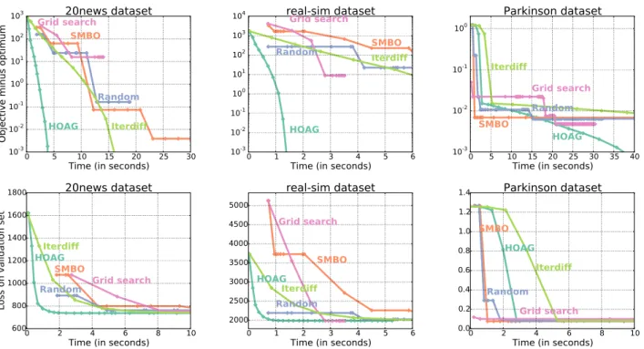
We report in Figure 3 the results of comparing the accu-racy of these methods as a function of time. Note that it is expected that the different methods have different starting points. This is because Grid Search and SMBO naturally start from a pre-deﬁned grid that starts from the extremes of the interval, while random search simply chooses a random point from the domain. For HOAGand Iterdiff, we take the

initialization λ1= 0.

In the upper row of Figure 3 we can see the suboptimal-ity of the different procedures as a function of time. We observe that HOAGand Iterdiff have similar behavior,

al-though HOAG features a smaller cost per iteration. This

can be explained because once HOAGhas made a step it can

use the previous solution of the inner optimization problem as a warm-start to compute the next gradient. This is not the case in Iterdiff since the computation of the gradient relies crucially on having sufﬁcient iterations of the inner optimization algorithm.

We note that in the Parkinson dataset, solution is inside a region that is almost ﬂat (the different cost functions can be seen in Figure 1 of the supplementary material). This can explain the difﬁculty of the methods to go beyond the 10−2 _{suboptimality level. In this case, SMBO, who starts}

by computing the cost function at the extremes of the do-main converges instantly to this region, which explains its fast convergence, although it is unable to improve the ini-tially reached suboptimality.

Suboptimality plots are a standard way to compare the per-formance of different optimization methods. However, for the context of machine learning it can be argued that es-timating hyperparameters up to a high precision is

(8)

unim-� � ��

Figure 3.Hyperparameter optimization methods. Top row: suboptimality of the different methods in terms of the test loss. Bottom row: loss measured on a validation set for the different methods.

portant and that methods should be compared in terms of generalization performance. In the lower row of Figure 3, we display the test loss (g) on a validation set, that is, using a third set of samples {(˜bi, ˜ai)}ri=1which is different from

both the train and test set. This ﬁgure reveals two main ef-fects. First, unsurprisingly, optimization beyond 10−2 _of

relative suboptimality is not reﬂected in this metric. Sec-ond, the fast (but noisy) early iterations of HOAGachieve the fastest convergence in two out of three datasets.

4. Discussion and future work

In previous sections we have presented and discussed sev-eral aspects of the HOAG algorithm. Finally, we outline some future directions that we think are worthwhile explor-ing.

Given the success of recent stochastic optimization tech-niques (Schmidt et al., 2013; Johnson and Zhang, 2013) it seems natural to study a stochastic variant of this algo-rithm, that is, one in which the updates in the inner and outer optimization schemes have a cost that is independent of the number of samples. However, the dependency on the Hessian of the inner optimization (∇2

1h) in the implicit

equation (2) makes this non-trivial.

Little is known of thestructure of solutions for the hyper-parameter optimization problem (HO). In fact, assumption

(A3) is introduced almost exclusively in order to guarantee existence of solutions. At the same time recent progress on the setting of image restoration, which can be considered a subproblem of (HO), has given sufﬁcient conditions on the input data for such solution to exist in an unbounded domain (De los Reyes et al., 2015). The characterization of solutions for the HO problem can potentially simplify the assumptions made in this paper.

The analysis presented in this paper can be extended in sev-eral ways. For instance, the analysis of HOAGis provided

for a constant step size and not for theadaptive step size strategy used in the experiments. Also, we have focused on proving asymptotic convergence of our algorithm. An interesting future direction would be to studyrates of con-vergence, which might give insight into an optimal choice for the tolerance decrease sequence.

Although we found the method to be quite robust in prac-tice, there are situations where it can get stuck in flat re-gions. For example, if the initial step is too big, it might land in a region with a large regularization parameter where the curvature is amost zero (hence the reason to normalize the first step by its norm). An interesting direction of fu-ture work is to make the method robust to such flat regions, scaping from flat regions and allowing the method to make bigger steps in early iterations.

(9)

Acknowledgments

I am in debt with Gabriel Peyr´e for numerous discussions, suggestions and pointers. I would equally like to thank the anonymous reviewers for many insightful comments, and to Justin Domke for posting the code of his Iterative differ-entiation method.

Feedback and comments are welcome at the author’s blog (http://goo.gl/WoV8R5).

The author acknowledges financial support from the “Chaire Economie des Nouvelles Données”, under the aus-pices of Institut Louis Bachelier, Havas-Media and Univer-sité Paris-Dauphine (ANR 11-LABX-0019).

References

Yoshua Bengio. Gradient-based optimization of hyperpa-rameters. Neural computation, 12(8):1889–1900, 2000. James Bergstra and Yoshua Bengio. Random search for

hyper-parameter optimization. The Journal of Machine Learning Research, 13(1), 2012.

James S. Bergstra, Rémi Bardenet, Yoshua Bengio, and Balázs Kégl. Algorithms for hyper-parameter optimiza-tion. In Advances in Neural Information Processing Sys-tems 24. 2011.

Eric Brochu, Vlad M Cora, and Nando De Freitas. A tu-torial on bayesian optimization of expensive cost func-tions, with application to active user modeling and hierarchical reinforcement learning. arXiv preprint arXiv:1012.2599, 2010.

Luca Calatroni, Cao Chung, Juan Carlos De Los Reyes, Carola-Bibiane Sch¨onlieb, and Tuomo Valkonen. Bilevel approaches for learning of variational imaging models. arXiv preprint arXiv:1505.02120, 2015. Olivier Chapelle, Vladimir Vapnik, Olivier Bousquet, and

Sayan Mukherjee. Choosing multiple parameters for support vector machines. Machine learning, 2002. Alexandre d’Aspremont. Smooth optimization with

ap-proximate gradient. SIAM Journal on Optimization, 2008.

J.C. De los Reyes, Carola-Bibiane Sch¨onlieb, and Tuomo Valkonen. The structure of optimal parameters for image restoration problems. arXiv preprint arXiv:1505.01953, 2015.

Charles-Alban Deledalle, Samuel Vaiter, Jalal Fadili, and Gabriel Peyr´e. Stein unbiased gradient estimator of the risk (SUGAR) for multiple parameter selection. SIAM Journal on Imaging Sciences, 2014.

Justin Domke. Generic methods for optimization-based modeling. In International Conference on Artiﬁcial In-telligence and Statistics, 2012.

Chuan-Sheng Foo, Chuong B. Do, and Andrew Y. Ng. Ef-ﬁcient multiple hyperparameter learning for log-linear models. In Advances in Neural Information Processing Systems 20. 2008.

Michael Friedlander and Mark Schmidt. Hybrid deterministic-stochastic methods for data ﬁtting. SIAM Journal on Scientiﬁc Computing, 2012.

Nicholas J Higham. Accuracy and stability of numerical algorithms. 2002.

Rie Johnson and Tong Zhang. Accelerating stochastic gra-dient descent using predictive variance reduction. In Ad-vances in Neural Information Processing Systems, 2013. Karl Kunisch and Thomas Pock. A bilevel optimization approach for parameter learning in variational models. SIAM Journal on Imaging Sciences, 2013.

Alexandre Lacoste, Hugo Larochelle, Franc¸ois Laviolette, and Mario Marchand. Sequential model-based ensemble optimization. arXiv preprint arXiv:1402.0796, 2014. Jan Larsen, Lars Kai Hansen, Claus Svarer, and M

Ohls-son. Design and regularization of neural networks: the optimal use of a validation set. In Proceedings of the IEEE Signal Processing Society Workshop. IEEE, 1996. Jan Larsen, Claus Svarer, Lars Nonboe Andersen, and Lars Kai Hansen. Adaptive regularization in neural net-work modeling. In Neural Netnet-works: Tricks of the Trade. Springer, 1998.

Chih-Jen Lin, Ruby C Weng, and S Sathiya Keerthi. Trust region newton method for logistic regression. The Jour-nal of Machine Learning Research, 2008.

Dong C Liu and Jorge Nocedal. On the limited memory bfgs method for large scale optimization. Mathematical programming, 1989.

Wei Liu and Yuhong Yang. Parametric or nonparametric? a parametricness index for model selection. The Annals of Statistics, 2011.

Dougal Maclaurin, David Duvenaud, and Ryan P. Adams. Gradient-based hyperparameter optimization through re-versible learning. In Proceedings of the 32nd Interna-tional Conference on Machine Learning, July 2015. Colin L Mallows. Some comments on Cp. Technometrics,

(10)

Yurii Nesterov. Introductory lectures on convex optimiza-tion. Springer Science & Business Media, 2004. Jorge Nocedal and Stephen Wright. Numerical

optimiza-tion. Springer Science & Business Media, 2006. Peter Ochs, Ren´e Ranftl, Thomas Brox, and Thomas Pock.

Bilevel optimization with nonsmooth lower level prob-lems. In Scale Space and Variational Methods in Com-puter Vision. Springer.

Neal Parikh and Stephen Boyd. Proximal algorithms. Foundations and Trends in optimization, 2013.

Barak A Pearlmutter. Fast exact multiplication by the hes-sian. Neural computation, 1994.

R Tyrrell Rockafellar and Roger J-B Wets. Variational analysis. Springer Science & Business Media.

Mark Schmidt, Nicolas Le Roux, and Francis R Bach. Con-vergence rates of inexact proximal-gradient methods for convex optimization. In Advances in neural information processing systems, 2011.

Mark Schmidt, Nicolas Le Roux, and Francis Bach. Mini-mizing ﬁnite sums with the stochastic average gradient. arXiv preprint arXiv:1309.2388, 2013.

Matthias W Seeger. Cross-validation optimization for large scale structured classiﬁcation kernel methods. The Jour-nal of Machine Learning Research, 2008.

Charles M Stein. Estimation of the mean of a multivariate normal distribution. The annals of Statistics, 1981. Kevin Swersky, Jasper Snoek, and Ryan Prescott Adams.

Freeze-thaw bayesian optimization. arXiv preprint arXiv:1406.3896, 2014.

Robert Tibshirani. Regression shrinkage and selection via the lasso. Journal of the Royal Statistical Society. Series B (Methodological), 1996.

Athanasios Tsanas, Max A Little, Patrick E McSharry, and Lorraine O Ramig. Accurate telemonitoring of parkin-son’s disease progression by noninvasive speech tests. Biomedical Engineering, IEEE Transactions on, 2010.