Newtoning financial development with heterogeneous firms

Newtoning financial development with

heterogeneous firms

Rafael CEZAR12 3

November 2011

Abstract: This article theoretically and empirically tests the link between financial constraints and the extensive

(proportion of exporters) and intensive (volume of exports) margins of international trade. The article's main contribution is its macroeconomic analysis of this relationship, which is further reaching than the sector-based focus found in the current literature. It also presents new information on firm behavior under financial constraints. The paper develops a trade model with heterogeneous firms and shows that countries with a high level of financial development have a lower productivity cut-off above which firms export and a higher proportion of exporting firms. Nevertheless, financial development is not correlated with firms' export volumes once they become exporters. An empirical analysis is developed on the basis of an international trade database on 135 countries between 1994 and 2007. The empirical analysis estimates a two-step gravity equation using panel data and confirms the first theoretical proposition that finance has a positive impact on the extensive margin. However, the intensive margin results are striking. They find a negative relationship between financial development and trade flows, confirmed by all the sensitivity tests. Despite the positive effect of financial development found by the literature in some economic sectors, the macroeconomic impact on overall exports was negative during the analyzed period.

Keywords: heterogeneous firms, trade, financial development. Classification JEL: F12, G20, 016.

1 _{Université Paris Dauphine, Place du Maréchal de Lattre de Tassigny, 75775 Paris Cedex 16, France. E-mail :}

rafael.cezar@dauphine.fr or rafael.cezar@yahoo.fr.

2 _{IRD UMR 225 DIAL}

Introduction

This paper aims to theoretically and empirically demonstrate the potential relationship between firms' financial constraints and the extensive and intensive margins of international trade. The first margin is the proportion of exporting firms and the second is the total volume exported by countries. In other words, the paper studies the link between financial development and international trade. Its main contribution is a macroeconomic analysis of the effect of financial development on trade, which paints a broader picture than the sector-based focus found in the specialized literature. The article also provides new insight into exporting firms' behavior under financial constraints. Lastly, it uses a new specification of the gravity model, as proposed by Helpman, Melitz and Rubinstein (2008), based on panel data.

Since the 1990s, there have been many studies of the effects of financial development on a number of macroeconomic variables. The focus initially was on the link between finance and economic growth, with King and Levine (1993) rekindling the debate by showing that financial development is closely connected with real GDP growth, rising investment rates and better physical capital performance. A number of articles have followed up on this analysis. Among them, Rajan and Zingales (1998) test and confirm the proposition that financial development is more beneficial to industries dependent on external finance and that these industries therefore post higher growth rates in countries where the financial industry is more developed.

Several authors also confirm this relationship. According to most sources, there are many channels for the link between finance and growth. First, there is the effect of financial intermediation on the use of savings, on its allocation to the most efficient investment project, and then on the production of information about these projects. Financial systems influence growth in terms of exercising corporate governance and monitoring investment projects. They facilitate trade in goods and financial transactions among economic agents. Lastly, financial intermediation influences growth by sharing, diversifying and managing risks (Levine, 2005).

Literature on the financial effect on international trade appeared much later, with Beck (2002) among the pioneers. He empirically tests a Heckscher-Ohlin model, developed by Kletzer and Bardhan (1987), which discusses the role of credit market imperfections in international specialization. The model predicts that financially developed countries specialize in manufacturing sectors rather than in agricultural sectors. The studies that followed were influenced by Rajan and Zingales and test the proposition that financially developed countries have a comparative advantage

in industries intensive in external finance (see Beck 2003, Svaleryd and Vlachos 2005; Hur et al., 2006). A new wave of literature appeared with the work of Chaney (2005) and Manova (2008) as firms' heterogeneity entered the debate.

The first author constructs a model of heterogeneous firms based on Melitz (2003). Firms are subject to financial constraints to pay export costs. The only firms that export are those whose profit, added to a liquidity shock, is higher than their exporting costs. Chaney demonstrates that there is a non-empty set of firms that are productive enough to export, but that do not export because of credit constraints. The second paper develops a similar model, but this time based on Helpman, Melitz and Rubinstein (2008). Manova shows that financial development is positively correlated with the extensive and intensive margins of trade and that this relationship is stronger in financially dependant industries. The empirical tests confirm her assumptions.

This paper continues the discussion and analyzes the macroeconomic effects of financial development on trade margins. I focus on identifying the effects of financial development on total trade to gain a broader picture than the sector-based effects sought by the literature. A theoretical model is constructed and then tested empirically.

Firms are heterogeneous by their productivity level and face fixed costs to export. Only firms that are productive enough to afford these costs can access foreign markets. I assume that firms finance all fixed costs via financial systems4. Credit markets are imperfect and this complicates the firms' access to external finance. Differentiating countries by their financial constraint level, the model finds that a higher proportion of firms export in financially developed countries. However, the volume exported by firms does not suffer from variations in financial level once they have become exporters. Therefore, the model does not determine a clear relationship between financial development and the intensive margin of trade. Two propositions are established. One is that financial systems have a positive effect on the extensive margin and the second tells that the relationship between financial development and the intensive margin is unclear.

An empirical analysis follows the model. These theoretical propositions are tested by the use of a sample of annual trade data covering 135 countries between 1994 and 2007. The financial constraint is measured by the ratio of total credit to the private sector and GDP.

4

To test the first theoretical proposition, I analyze the ratio of the productivity of the most productive firms to the productivity cut-off above which firms export (see equation 12). If it is higher than 1, at least one firm is productive enough to export, but if it is less than 1, no firm exports. Despite the lack of data on productivity levels and on their distribution, the existence or non-existence of trade is noticeable, and so the role of financial development on firm selection can be tested using a probit model. The results confirm the hypothesis and show that financial development lowers the productivity cut-off and raises the proportion of exporting firms.

The use of macroeconomic data for this estimate is possible because the characteristics of firms' exporting decisions can be identified from the analysis of the marginal variation of the data. Therefore, the gravity model framework is used for the estimates.

Subsequently, I test the effects of finance on the intensive margin by estimating a two-step gravity model. The first step is the estimate of the extensive margin and the second is the estimate of trade flows using a traditional gravity equation controlling for the endogenous proportion of exporting firms (see equation 18)5.

The main empirical results are striking. The coefficient of the financial variable is negative and significant for both tested specifications. This indicates that, over the fourteen years, the increase in financial development caused the reduction in total exports, all sectors together.

To evaluate the robustness of these results, I conduct a wide range of sensitivity tests. I test the independence of the relationship and control for a possible omitted variable bias. To reduce the possibility of simultaneous adjustments and ensure that a reverse causality bias does not distort the results, I use a moving average for the financial indicator. I check the influence of outliers and also test the linearity of the financial variable. Lastly, I use other indicators to measure financial development. Subsequently, to test the robustness of the control function to the extensive margin, I relax the distribution assumption about firms' productivity and estimate a polynomial model. All these tests turn up merely marginal variations in the financial coefficient, which remains negative and significant.

The specialized literature points to a positive relationship between financial development and exports in industries dependent on external finance. The results in this paper are therefore

5

complementary to this finding. It shows that the overall effect is negative and financial development reduces total exports. This find can be explained by the decrease in exports in some sectors that offsets the export growth driven by financial development in financially vulnerable industries. The

finance – intensive margin relationship takes two distinct paths: financial development induces a

reduction in total trade, as shown by this article, and, on the other hand, provokes a comparative advantage in financially vulnerable sectors, as shown by the literature.

There is a strong link between financial development and the extensive margin. However, the effects of finance on the intensive margin are ambiguous and depend mainly on each industry.

1) Theoretical model

This model seeks to clarify the relationship between financial development and countries' total trade. I introduce financial constraints into the Helpman, Melitz and Rubinstein model (2008), as in Manova (2008), but without differentiating between economic industries. Firms face fixed costs to export and finance all of them externally. Credit markets are imperfect and complicate the financing of these costs. The model differentiates countries by their levels of financial constraints to show that financial development raises the proportion of exporting firms. However firms' export volumes are independent of the financial constraint level once the trade relationship is established. The main findings are that financial development is positively correlated with the increase in the extensive margin, but its effect on the intensive margin is uncertain. The link between finance and trade channels through the extensive margin.

Set-up of the model

I consider a simple analytical framework with i countries and one single industry, composed of Ni

heterogeneous firms in each country. Each firm produces a single variety of good, so they are monopolistic in their variety. Consumers like variety and they consume all goods on offer. They share the same preferences, represented by a constant elasticity of substitution (CES). The utility function of country i is the sum of all individual CES functions:

α α ω

ω

ω

1 ) ( _       =

_∫

Ω ∈ d q U i i i

where parameter α defines the constant elasticity of substitution across products, which equals ε = 1/(1- α), 0 < α < 1 and so ε > 1. Country i's consumption of variety ω is denoted qi(ω) and Ωi is the

set of all available varieties in this country. Each variety in the set is offered at price pi(ω). The ideal

price index is:

ε ε ω

ω

ω

− − Ω ∈         =

_∫

1 1 1 ) ( d p P i i i (1)

If Yi is the total income of country i, demand for the variety ω equals:

i i i Y P p q _      =

ω

_−ε−ε

ω

1 ) ( ) ( (2)

Production and trade costs

In line with Melitz (2003), firms face sunk costs to enter the domestic market. Only after entry that they learn their productivity level, which determines their profit level. To produce, firms use a combination of inputs and the cost of this combination to produce a unit of good is ci, which is the

output of a cost minimization program and is specific to each country.

Firms are heterogeneous by their productivity level, noted φ. Productivity follows a cumulative distribution function µ(φ) with supports [φB , φH] and φH > φB > 0, where φH is the productivity of

the most productive firm and φB is the productivity of the less productive.

Firms have a cost function with constant returns. The unit cost of production in country i is ci/φ

where 1/φ measures the inputs used to produce a unit of good. Note that ci is specific to each

country and it reflects differences between input prices across countries. In the other hand, φ is specific to each firm and captures heterogeneity between them. I assume that µ(φ) is the same across countries and, therefore, differences in productivity levels across countries are captured by ci.

Firms do not face fixed costs to produce for the domestic market. After paying the sunk cost, all firms can produce and sell on the domestic market. This simplification enables a focus on the firms' export decisions.

If firms export, they face two different costs: a fixed cost and a variable cost. The first one is specific to each country-pair and is the same for all firms. I denote cifij as the fixed cost to export

from country i to country j, expressed in units of the factors bundle and normalized by the input cost. fij > 0 for all i ≠ j and fij = 0 if i = j. The variable costs take the form of an iceberg trade cost

and τij > 1 unit of goods are shipped by country i for 1 unit delivered to the destination. The total

cost to export q units from i to j is:

ij i i ij ij ij c f c q q c _+      =

ϕ

τ

) (

Financial constraints and trade

Firms face many costs to export, which should normally be payed before the start of the trade relationship, i.e. before profits are made. Unconstrained models assume that firms face no financial constraints to finance these costs. However, if financial systems are imperfect, another equilibrium should be calculated.

Fixed costs in international trade are highly diverse. They consist, for example, of investments to adapt production to a new market and new customers. Firms also need to seek new partners on foreign markets, pay translation costs, and comply with local legislation and local standards. Long lead-times between shipping and delivery are also a heavy burden. Additional difficulties are added to the magnitude of these costs because foreign activities are normally riskier than domestic ones. Firms also have to contend with exchange rate, protectionist and political risks.

Subsequently firms' fixed export costs are large and risky, and firms need the financial system to finance these costs. If the financial system is fully efficient, equilibrium is the same as in the unconstrained model. But if the financial system is imperfect, firms have to contend with financial constraints to access external finance and export.

To model the effects of financial constraint on trade, I assume that the level of financial constraints varies between countries and that the characteristics of each system determine the firms' access to external finance and risk management. Firms use the financial systems to finance their entire fixed

export costs6 and I also assume that firms self-finance their variable costs without any difficulty (the results remain the same if this assumption is relaxed).

The export procedure is as follows: First firms seek the financial system to finance their fixed export cost. They already know their prices and the demand for each variety and therefore they are familiar with the export earnings and costs. Firms with enough net earnings (earnings minus variable costs) to pay for the loan borrowed in the first period, plus the cost of using the financial system, get the credit and export. In the last period, exporters refund the loan. Firms with lower forecast net earnings than the loan do not export.

Financial constraints are heterogeneous between countries. Each country has a different level of financial development, which is exogenous and denoted ϴi. To simplify, I assume 0 ≤ ϴi ≤ 1, where

ϴi equals 1 when firms have no constraints on their access to credit and it equals zero otherwise.

This index shows the level of financial development and so how firms access external finance.

To export to country j, firms in country i are subject to the following constraint:

ϕ

τ

ϕ

ϕ

ϕ

θ

i ij ij ij ij ij i i c q p q f c f( ) ≤ ( ) ( )− ( ) where ( )<0 ∂ ∂ θθ f

where f(ϴi) is the cost of using external finance in country i. I assume that f(ϴ=1) = 1 and that f(ϴ)

is a strictly monotonic and continuous function, decreasing with ϴ. That means that an increase in the level of financial development reduces the cost of external finance. f(ϴi)cifij is the amount due at

the end of the period, which must be at least equal to the firm's net earnings, otherwise firms cannot export.

Equilibrium with financial constraints

Equilibrium is characterized by a productivity cut-off above which firms export. Firms export if the activity is profitable, i.e. if their profit from exporting is at least equal to zero. Each producer is monopolistic in their variety and hence the equilibrium price is a mark-up of the variable cost. An exporter with productivity level φ knows the demand from country i and sells its variety to this country at price:

6

ε ε

αϕ

τ

ϕ

₋ −       = ₁ ) ( j j i ij ij P Y c q and

αϕ

τ

ϕ

τ

ε

ε

ϕ

ij i ij i ij c c p  =      − = 1 ) (

The earnings from sales to this country equal:

j j ij j j i ij ij Y P p Y P c r ε ε

ϕ

αϕ

τ

ϕ

− −         =         = 1 1 ) ( ) ( (3)

And the profit function of this exporter is:

(

)

j i i ij j ij ij Y f c f P p ) ( ) ( 1 ) ( 1

θ

ϕ

α

ϕ

ε −         − = Π − (4)

The productivity cut-off above which firms export in the constraint model is noted φ*. Only firms with productivity level above φ* can export. The cut-off is defined by the zero profit condition below:

0 *)

( =

Π ϕ (5)

This cut-off is country-pair specific and only firms with productivity higher than

ϕ

_ij* can export from country i to country j.

Unfortunately, the productivity level is not easily observable. But as the firm's earnings are increasing with productivity, I use the earnings function as a proxy for firms’ productivity level. The earnings cut-off above which firms export from country i to j is:

(

i i ij

)

ij i i j j ij ij ij ij f c f f c f Y P p r ( ) 1 ) ( ) ( ) ( 1 * * ε θ α θ ϕ ϕ ε = − =         = − (6)

Only firms with earnings greater than rij(φ*) export. This threshold is increasing with f(ϴ), and

when the financial system develops, f(ϴ) decreases, as does the productivity cut-off. This enables firms with a lower productivity index to access international markets. Hence a higher proportion of firms are able to export in financially developed countries.

Financial constraints and the trade margins

The extensive margin is the proportion of exporting firms. Given that firms' export decisions are based on the analysis of their profit function, the extensive margin is represented theoretically by

the productivity cut-off. When this threshold decreases, the proportion of exporting firms increases.

The relationship between finance and the extensive margin channels through the productivity cut-off. When the financial system develops, f(ϴ) decreases and the productivity cut-off is reduced. Firm selection broadens and less productive firms become exporters. This mechanism shows that financial development has a positive effect on the proportion of exporting firms. To demonstrate this effect, I calculate the elasticity of the productivity cut-off to the level of financial development:

0 *) ( * _< ∂ ∂ ≈ ∂ ∂ θ ϕ θ ϕ r because ( )<0 ∂ ∂ θθ f (7)

This elasticity is negative, confirming the inverse relationship between φ* and ϴ. This result shows that financial development is a determinant of the extensive margin of trade. The first theoretical proposition is defined as follows:

Proposition 1: Financial development is positively correlated with the extensive margin of trade such that when the financial system develops, a greater proportion of firms export.

To analyze the relationship between finance and the intensive margin, I define Vij as the endogenous

proportion of exporting firms. It is a function of the productivity distribution and the productivity cut-off, as below:     > ∫ ≤ = − H H ij if if d V H

ϕ

ϕ

ϕ

ϕ

ϕ

µ

ϕ

ϕ ϕ ε * 0 * ) ( * 1 (8)

If φ* > φH , then Vij = 0 because the productivity cut-off is higher than the productivity of the most

productive firm and no firm is productive enough to export7. If φ* < φH, then Vij > 0 and at least one

firm is productive enough to export. And when φ* decreases, the number of exporting firms increases. This variable is country-pair specific and I assume that Vij ≠ Vji 8.

The value of total exports from i to j is the sum of firms' individual exports. It is a function of the

firms' export earnings, the size of the country (measured by the number of firms) and the proportion of exporting firms. Xij is defined as follows:

7 _{Therefore V}

ij takes into account the zero-trade observations. 8

ij i j j i ij ij Y NV P c X ε

α

τ

−         = 1 (9)

The scale of Xij depends essentially on the volume of individual exports and on the extensive

margin, after controlling for country size. The first equals the export earnings of each firm and is not affected by the level of financial development. Effectively, as the productivity distribution function is the same for all countries and because prices are a constant mark-up of variable costs, individual export earnings are not affected by ϴ (see equation 3). Nevertheless, as the proportion of exporting firms is a positive function of ϴ, the link between finance and intensive margin channels through the extensive margin. However, once controlled for the endogenous proportion of exporting firms, the theoretical model does not suggest a clear relationship between financial development and trade flows. The second proposition is made:

Proposition 2: The theoretical effect of financial development on the intensive margin is unclear.

This assumption is true if proposition 1 is borne out.

2) Empirical model

A gravity equation is developed from the previous model to empirically test the theoretical assumptions. The gravity model is one of the most successful models in international economics and a number of specifications have already been tested. I follow Helpman et al. (2008) and estimate a two-step gravity equation with control for the extensive margin.

The log-linearization of equation 9 enables that total exports from country i to j can be written as follows: ij i j j ij i ij c P Y N V X (1 )ln (1 )ln ( 1)ln ( 1)ln ln ln ln ln = −ε + −ε τ + ε− α+ ε− + + + (10)

I assume that τij is a stochastic cost consisting of a country-pair's specific costs and an i.i.d trade

friction. I also assume that a uij

ij ij =D e

−ε

τ

1

, where Dij denotes the distance between the two countries

and uij ~ N(0,

2

u

σ

). Representing the logarithms with lower case letters, I rewrite equation 10:

ij ij ij j i ij aD v u x =

χ

0 +

χ

+

χ

+ + − (11)

and importing countries respectively. χi is the same for any country to which i exports and χj is

identical for all countries that export to j.

Equation 11 is very similar to a traditional gravity equation. However vij differentiates (11) from the

traditional models, such as that presented by Anderson and Wincoop (2003).

The role of financial systems in firms' selection

According to the theoretical assumptions, financial development lowers the productivity cut-off above which firms export. This enables less productive firms to access foreign markets. The financial system plays a role in firms' selection into export.

To study this relationship, I start by defining the latent variable Zij as the ratio of the productivity of

the most productive firm – φH – to the productivity cut-off specific to i j –

ϕ

ij*. If φH <

*

ij

ϕ

, the productivity cut-off is higher than the productivity of the most productive firm and no firms export from country i to j. But if φH >

ϕ

ij*, there is a set of firms whose productivity is above the

productivity cut-off, and these firms export. In the first case, Zij is less than 1, and in the second

case, Zij is necessarily greater than 1. This latent variable therefore reveals whether the two

countries trade, and it is defined as:

(

)

1 1 1 * ) ( − − − _       =         = ε ε ε

ϕ

θ

ε

τ

α

ϕ

ϕ

H ij i j i ij j ij H ij f f Y c P Z (12)

where fij denotes country-pair trade frictions and represents the specific trade costs to export from i

to j. I assume fij = exp(фi + фj + фij + υij) where υij ~ N(0,συ2). фi is a measurement of country i

export costs while фj denotes a common trade barrier to any country that exports to j, and фij is a

country-pair specific cost. Using these specifications and log linearizing (12), Zij can be expressed

as: ij i ij j i ij f z =γ0 +γ +γ +γ + (θ )+η (13)

where zij is the log of Zij. γi = фi-(1-ε)lnci and γj = фj-(ε-1)lnPj+lnYj represent the characteristics of

exporting and importing countries respectively. γij represents the fixed effect specific to the country

pair and ηij ≡ uij + υij ~ N(0, σu2+

2 υ

between them, and it can be used as a proxy for Zij. I define the dummy variable Tij as an indicator

of the existence of trade flows. Therefore, Tij = 1 if Zij > 0 and Tij = 0 if Zij < 0. As it is an

observable variable, I can estimate Zij from Tij. And as the disturbance ηij follows a normal law with

variance

σ

_η2, the standardization to the unit of this variance enables the estimation of Zij by a probit

model using Tij as the dependent variable. As Tij equals 1 when country i exports to j, then the

conditional probability that i exports to j – ρij – is given by the following probit equation:

(

)

(

)

(

i j ij i ij

)

ij ij ij f z T

η

θ

γ

γ

γ

γ

ρ

≥ + + + + = > = = = ) ( Pr variables observed 0 Pr variables observed 1 Pr 0 Defining Z_ij* as:

(

γ

γ

γ

γ

θ

)

ση 1 0 * ) ( i ij j i ij f Z =

I can then estimate the probability ρij using the following probit equation:

) ( _ij*

ij

β

z

ρ

=Φ (14) where zij* is the logarithm of

*

ij

Z and Φ(•) is the cumulative distribution function of a standard normal law.

This equation enables Zij to be estimated by a probit model using observable variables from the

exporting and importing countries. I can then analyze the effect of these variables on the existence of trade between two countries, more precisely the financial effect on the extensive margin. A positive coefficient indicates, for example, that a positive variation in the variable induces an increase in Zij, by reducing the productivity cut-off or by increasing firm productivity9. Therefore

the effect of financial development on firms' selection can be tested empirically.

It is important to note that the selection equation is derived from a firm-level decision, and shows how changes in country characteristics affect firms' incentives to export. However, it does not contain direct information on the endogenous proportion of exporting firms, but on its marginal variation. Moreover, equation 14 can be used to derive consistent estimates of Vij, as can be seen in

9

the next section.

Finance and the intensive margin

I draw on Chaney (2008) and assume that φ follows a truncated Pareto distribution10 and that its distribution function respects µ(φ) = (φk- k

B

ϕ

) / ( k H

ϕ

- k B

ϕ

), where k > (ε – 1). Equation 8 can thus be rewritten as:

(

)

(

)

ij k ij k B k H ij W k k V *( 1) 1 + − − + − = ϕ ε ϕ ϕ ε And:         −         = + − 0 , 1 1 * ε ϕ ϕ k ij H ij Max W

I next rewrite Vij as a monotonic function of Wij11. With these assumptions, this variable captures the

extensive margin or the endogenous number of exporting firms, and also the existence of trade between the two countries. As the distribution function of φ supports [φB , φH] and φH > φB > 0, if

φH <

*

ij

ϕ

, no firm is productive enough to export and Wij = 0, as Xij. And if φH >

*

ij

ϕ

, Wij (as a

monotonic function of Vij) captures the proportion of exporting firms. As Zij is the ratio of the

productivity of the most productive firm to the productivity cut-off, I can rewrite

      − = − + − 0 , 1 1 1 ε ε k ij ij Max Z W . If _ij ^

ρ

is the estimated probability that i exports to j,       Φ = − ij ij z ^ 1 * ^

ρ

and the endogenous proportion of exporting firms can be estimated from observed variables using the following equation:

10 _{Chaney (2008) argues that this distribution law is a good approximation of the true firm productivity distribution.}

Helpman et al. (2008) relax this distributional assumption and conclude that “Pareto distribution does not appear to

restrict the basic specification of the model”.

11 _{By substituting v}

ij with wij, the constant term of vij, precisely

(

)

(

)

       − + − k k_B k k H ϕ ϕ ε 1

        −       =         −       = 1, 0 1, 0 * ^ * ^ * ^ l l ij ij ij ij Max Z T Z W (15) where σ_η εε1 1 − + − = k l _.

Using these specifications, I estimate equation 11 in two steps. The first is the estimate of Wij

above, using information from the probit (14). In the second step, I estimate xij controlling for the

endogenous proportion of exporting firms, with wij calculated in the first step. Equation 11 can be

rewritten as follows: ij ij ij ij j i ij aD b w u x =

χ

0 +

χ

+

χ

+ + ln

ϕ

*+ −

where b = k – ε + 1. As the productivity cut-off is not observed, I use equation 6 to substitute it in the equation by β0 + (ε-1)lnPj + lnYj - εlnci - lnf(ϴ) + alnDij - uij + фi + фj + фij - υij, where υij ~ N(0,σ_υ2). I estimate the value of total exports from i to j as:

ij ij i ij j i ij f w e x =Ψ₀+Ψ +Ψ +Ψ + (θ )+ + (16)

where ψi = χi+εlnci+фi and ψj = χj+(ε-1)lnPj+фj represent trade barriers specific to countries i and j

respectively. The term ψij = aDij+фij denotes bilateral trade costs specific to the country pair i j. eij ~ N(0,σ_u2+σ_υ2) is an i.i.d. measurement error.

Estimation methodology

Under the financial constraint hypothesis, the development of financial systems plays a positive role in firms' selection into trade. It reduces the financial constraint, enabling a larger proportion of firms to export. To test this assumption, I estimate equation 14. As shown above, I use the traditional gravity equation's framework to estimate the probit equation below:

              + + + + + + + + + + + Φ = t t ij t ij t ij t ij t ij t ij t ij t t ij t t ij t t ij t j i t j i t t i t t ij Area Island Landlocked SameCtry Colony Lang Contig Currency WTO FTA Pop Y Dist

β

β

β

β

β

β

β

β

β

β

β

β

β

β

β

θ

β

ρ

0 14 13 12 11 10 9 8 , 7 , 6 , 5 , 4 , 3 2 1 , ln ln ln ln ln (17)

where i et j denote the exporting and importing countries respectively and t the year. Dist is the distance between two countries. Y is real GDP, Pop is the population and Area is the area in km2.

These are country-specific variables. FTA indicates the existence of a free trade agreement between

i and j. WTO equals 1 if the two countries in the pair are members of the World Trade Organization. Currency indicates whether i and j share a common currency. Contig, Lang, Colony and SameCtry

are dummy variables and, when equal to 1, indicate respectively a common border, a common language, a colonial link in the past and whether the two countries have been the same country in the past. Landlocked and Island indicate the number of landlocked countries and islands in the country pair12.

This empirical model uses an analytical gravity framework, with aggregate statistics, to analyze the microeconomic impact of heterogeneous firms' exporting decisions. This property results from the fact that the characteristics of marginal exporters (increase or decrease of the productivity cut-off) can be identified from marginal variations in the features of exporting and importing countries and in the observable trade costs. This is one of this approach's major advantages, since it enables the use of a macroeconomic framework to extract firm-level information, which would normally require a micro database.

I then analyze the impact of financial development on the intensive margin of international trade, by estimating equation 16. This equation is very similar to a traditional gravity equation, but with a control function for the extensive margin of trade. I estimate this equation in a two-step procedure.

In the first step, I estimate ij ,t

^

ρ

and calculate       Φ = − t ij ij z , ^ 1 * ^

ρ

and then wij can be estimated by

equation 15. The second step is the gravity equation below:

t ij t j i t ij t ij j i ij ij ij t ij t ij t ij t j i t j i ij t i t ij e z w Area SameCtry Colony Lang Contig Currency WTO FTA Pop Y Dist x , 0 * , ^ 14 * , ^ 13 , 12 11 10 9 8 , 7 , 6 , 5 , 4 , 3 2 , 1 , ln ln ln ln ln + Υ + Υ + Υ + Υ +       Υ Υ + Υ + Υ + Υ + Υ + Υ + Υ + Υ Υ + Υ + Υ + Υ + Υ =

λ

θ

(18)

where Υi, Υj and Υt represent respectively the controls for exporter and importer fixed effect and the

time fixed effect. _

     Φ       =       * , ^ * , ^ * , ^ / ijt t ij t ij z z z

φ

λ

is the inverse of the Mills ratio and Υ14 = cov (eij,t,

12

ηij,t)

σ

e2_ij,t.       Υ *, ^

14

λ

zijt is the normal procedure to control for selection bias since E(eij,t | xij,t > 0) ≠ 0, since zero-trade observations constitute almost 30% of the sample (see Heckman, 1979, and Wooldridge, 1995). The variable wij,t is also constructed with information from 17 and thus suffers

from a selection bias. Therefore I use

        −               Φ       + =ln exp / 1 * , ^ * , ^ * , ^ * ,t ijt ijt ijt ij z z z w l

φ

_{instead of wij,t}13_,

since w*ij,t is a consistent estimator of E(wij,t | .,Tij,t = 1) (see Santos Silva and Tenreyro, 2009).

Estimating 18, using the Heckman correction, calls for some strong assumptions about the model's parameters. Mostly about the normality assumption of the unobserved trade costs. A less restrictive control is the semi-parametric model, which entails the selection of some excluded variables (see Das, Newey and Vella, 2003). These variables should be correlated with the fixed costs, but they should not be directly correlated with eij,t. The fixed-effect model does not require such a

specification, since all time-invariant variables are already excluded. In all the other specifications, I exclude the exogenous variables Landlocked and Island.

3) Data

The empirical analysis uses an international database on trade between 135 countries. Data are annual and cover the period between 1994 and 2007. Trade data are taken from the International Monetary Fund's Direction of Trade Statistics. The data are in current and undeflated US millions of dollars. Each country pair has two distinct observations: exports from i to j and exports from j to i.

Data to measure Gross Domestic Product comes from two different sources: the IMF's World

Economic Outlook Database and the World Bank's World Development Indicators. Data are in

current US$ and are not deflated. The population variable was constructed using information from the World Bank's Health, Nutrition and Population Statistics rounded out with data from the Pen 13 Where _               Φ * , ^ / * , ^ t ij z t ij z

World Table (http://pwt.econ.upenn.edu/).

The distance variable is based on data weighted by the population's geographic distribution. This variable as well as Area and the dummy variables Contig, Lang, Colony, SameCtry and Landlocked, were taken from the CEPII Distance database (http://www.cepii.fr/francgraph/bdd/distances.htm).

The Free Trade Agreements variable was constructed entirely from World Trade Organization information on regional trade treaties (data are available on the website: http://rtais.wto.org/UI/PublicSearchByCr.aspx). By regional treaties, I mean free trade agreements and customs unions. The WTO variable was also constructed from information available on the WTO website (http://www.wto.org/english/thewto_e/gattmem_e.htm and http://www.wto.org/english/thewto_e/whatis_e/tif_e/org6_e.htm). Currency comes from an update of the database provided by Glick & Rose (2002)14.

Financial development

Levine (2005) states that financial development reflects the balance between savers and borrowers and the maximization of their interest. To promote this equilibrium's efficiency, the system must properly fulfill the functions of savings mobilization, capital allocation, risk management, firm monitoring and information sharing. In this context, a good financial indicator would ideally be sensitive to the efficiency of intermediaries at fulfilling all these functions. However, such measures are unfortunately not available for a sufficient number of countries to be able to conduct an international comparative study. Therefore, I follow the literature and use the most traditional financial development indicator: Private.

The indicator is a measure of the amount of credit granted to the private sector. More specifically, it equals the ratio of private credit provided by deposit money banks and other financial institutions to GDP. It is an important indicator because it measures the relative amount of loans allocated to the private sector, so it provides a good measurement of the financial constraints faced by firms. The lowest value of this indicator is zero, which indicates an economy with no private credit. An increase in the indicator points to the development of the financial system.

14 _{I also use their definition of monetary union: the exchange rate between two currencies is fixed or unchanged so that}

Data on this variable are available for the 14 years and the 135 selected countries. Data are provided by the World Bank. I use two different sources: the database provided by Beck, Demirguc-Kunt and Levine(2000)15, and the Global Development Finance database.

4) Estimating trade margins

In this section, I use the empirical model presented above to test the two theoretical assumptions. More precisely, I empirically test the link between financial development and the extensive and intensive margins of trade.

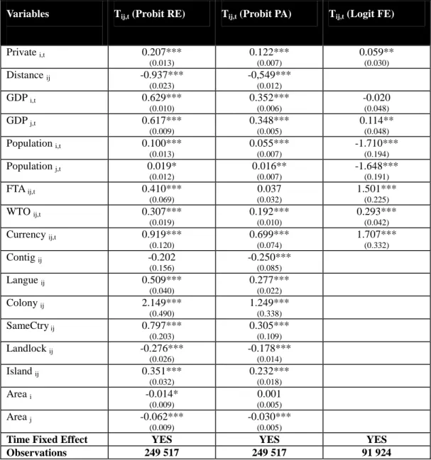
I first test the theoretical assumption of the positive effect of finance on the extensive margin. This hypothesis states that when the financial constraint is relaxed, the productivity cut-off above which firms export is lowered and a greater proportion of firms are able to export. To test this assumption, I estimate equation 17 using a probit model with the traditional gravity framework as explanatory variables to control for country features and trade costs. Like Berthou (2010), I estimate equation 17 using a Random Effect Probit model and I control for time effects using time dummies. To test the robustness of the results under this specification, I also estimate equation 17 using a Probit Population Averaged model and a Fixed Effect Logit model, both with panel data. Results are presented in Table I16.

The first column shows the coefficients for the Probit Random Effect model. The dependant variable is a dummy variable that indicates whether the country pair trade (Tij = 1) or not (Tij = 0).

All the traditional control variables have the expected sign, which demonstrates a good fit of the model. The Distance coefficient is negative and indicates that a positive variation in this variable reduces the probability of two countries trading and reduces zij. In other words, an increase in

distance raises trade costs and increases the productivity cut-off above which firms export17. This,

15

I use the database updated in April 2010.

16 _{These estimates use panel data to simplify the presentation of the results. However, despite this panel estimate, I}

draw on Wooldridge (1995) to construct the control function for the selection bias and the extensive margin in the estimation of the intensive margin. That means that I use a different coefficient for each of the 14 years to the construction of Zij.

17 _{Or reduces φ}

in turn, reduces the proportion of exporting firms. The GDP coefficients are positive, as expected. The analysis also turns up a positive correlation between a firm's selection into trade and membership of a free trade zone, World Trade Organization membership and sharing a common currency. All these variables reduce trade costs and therefore reduce zij by reducing the productivity

cut-off. And thus this mechanism plays a positive role in firm selection. The effect of a common border is the only exception: despite its effect on the reduction of trade costs, this variable has a negative coefficient. I attribute this result to the effect of border conflicts, which stem trade between neighbors.

As expected by the theoretical assumption, the financial indicator coefficient is positive and significant. It shows that a positive variation in Private raises zij by reducing the productivity

cut-off. This allows that less productive firms export, meaning that a higher proportion of firms can export. The results confirm the first theoretical proposition.

I then estimate 17 using a Probit Average Population model, also with panel data. The results are presented in the second column of the table. In general, all the coefficient values are lower than with the random effect model, but they have both the same sign and are significant. The financial indicator is positive and significant at 1%, confirming the previous result. The third column shows 17 estimated using a Logit Fixed Effect model18. The Private coefficient is also positive under this specification, confirming the positive role of financial development in firm selection into export19. When financial constraints are eased, a higher proportion of firms access foreign markets.

Next, I estimate a gravity equation to test the second theoretical assumption. The model suggests that the link between finance and trade goes through firm’s selection into export. However, once firms have become exporters, the value of their exports is not affected by the level of financial constraints. The theoretical model, therefore, puts forward an unclear relationship between financial development and the intensive margin of trade. I test this relationship by estimating equation 18 using a two-step gravity model with panel data. The first stage is the previous probit equation. I

18 _{Despite the change in distribution hypothesis, the probit and logit estimators are very similar, which makes it}

possible to test the robustness of the results using a fixed effect model.

19 _{Nevertheless, it is not interpreted in the same way as with the other two models, because this model estimates the}

within variance. As the dependent variable is a dummy, the fixed effect coefficient indicates the probability of switching from exporter to non-exporter and vice versa. Therefore, the sample is reduced by about a third since it includes only the country-pairs whose dependent variable has changed from 0 to 1 or otherwise.

then use these results to calculate w*ij,t20 and then I estimate the trade flows, controlling for the endogenous proportion of exporting firms using.

The log-linearization of (18) enables the estimate of the equation using an ordinary least squares (OLS) model. As about 30% of the sample comprises zero-trade observations, this specification suffers from a selection bias because the conditional expectation of the error term is not zero, which means that E(eij,t|xij,t>0) ≠ 0. I control for this bias by introducing the inverse Mills ratio. I also

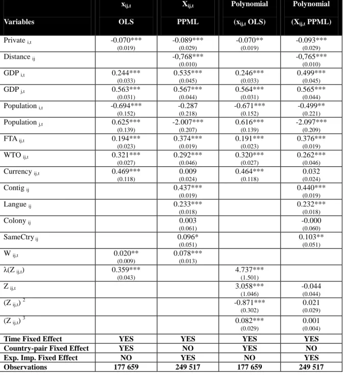
estimate the relationship using a non-linear model to control for the robustness of the results. I follow Silva and Tenreyro (2009) and I use the Poisson Pseudo Maximum Likelihood model21. As the data are in panel, the two specifications use the fixed-effect model (Anderson and Wincoop, 2003) and I control for the time effect. The results are given in the first two columns of Table II. The first column presents the OLS coefficients and the second column the PPML model. The standard deviations are robust in the two specifications22 and the dependent variable is total exports from country i to j in the non-linear specification and its log in the linear model.

The coefficients of the control variables have the expected sign and show a good fit of the model. The variables of Distance, Common Border, Language, Colony, SameCtry and Area were not estimated in the linear model because they are all time invariant. Nevertheless, their coefficients have the expected sign in the non-linear model. GDP is positive and significant in the two specifications, indicating that increases in these variables raise export value. The Free Trade

Agreement variable is positive and confirms the hypothesis that trade agreements raise trade value. WTO is also positive, as is Currency, indicating that membership of the World Trade Organization

20 _{As in the empirical model, I calculate}

        −                 Φ         + =ln exp / 1 * , ^ * , ^ * , ^ * ,t ijt ijt ijt ij z z z

w l φ _{to control for firm}

heterogeneity. I calculate this statistic from 

     Φ = − ij ij z ^ 1 * ^

ρ . However, the data characteristics complicate this calculation: the sample includes a relatively small number of country pairs whose characteristics are such that their probability of trade is indistinguishable from 1. Differences in z*_ij are so not observable in the sample as a function of ρij,t. Therefore, I attribute the same

*

ij

z for these country pairs as ρij,t >0,999999, which represents about 4.03% of

the sample.

21 _{The dependent variable in this specification is not in log and therefore all the observations are estimated. In this}

case, there is no selection bias and the Heckman correction is not used.

22 _{I use the cluster and robust option in the estimate. The bootstrap method does not change the significance of the}

and sharing the same currency both increase trade flows. These results confirm the recent gravity literature, even using this new gravity specification (see, for example, Baier & Bergstrand, 2007; Rose, 2004; and Glick & Rose, 2002).

The control function for extensive margin wij,t has a positive coefficient, as expected (see Chaney,

2008), and shows that an increase in the proportion of exporting firms generates a positive variation in export volume. wij,t is also significantly different from zero. This finding demonstrates the

robustness of this control and the importance of the extensive margin to the estimate of a gravity model.

The financial indicator Private has a negative coefficient in both specifications tested. It measures financial development and the results find that a positive variation in the level of financial development during the analyzed period induced a negative variation in trade flows, after controlling for the endogenous proportion of exporting firms. In other words, the results find a negative elasticity between trade flows and financial development. The two coefficients are significant at 1%.

I then relax the parametric hypothesis about the pareto distribution of firm productivity in equation 8. Using equations 6 and 12, I assume that ѵij ≡ ξ(zij) is an increasing function of zij. The controlling

function for the extensive margin in equation 18 is switched from w*ij,t to ξ(z*_ij,t), which I

approximate with a polynomial in z_ij*_,t. I re-estimate equation 18 for the linear and non-linear models using this new polynomial function to control for the endogenous proportion of exporting firms. The results are presented in the third and fourth columns of Table II23.

The changes in the coefficients and in the standard deviation are marginal under this new specification and the new results are very similar to the parametric model. The financial indicator is negative and significant at 1%, as it was before. This new specification confirms the previous results and indicates a negative relationship between financial development and international trade flows, after controlling for the extensive margin.

Two recent papers are consistent with these main findings. Berman and Héricourt (2010) analyze a sample of 5,000 firms in nine developing countries. They observe a disconnection between financial

23

development and the intensive margin of trade, despites a positive relationship between firms' access to credit and their export decision. Muûls (2008) presents similar findings using microdata from 9,000 Belgian firms between 1999 and 2005. He finds a positive effect on the extensive margin and his estimates suggest a vague and insignificant effect of financial development on the intensive margin. The authors conclude that once firms become exporters, credit constraints affect neither their export value nor their growth.

Unlike these results, the core body of literature24 finds a positive relationship between finance and the intensive margin of trade. Yet this literature analyzes the relationship differentiating the economic sectors by their level of dependence on external finance. This paper studies the macroeconomic effects of financial development on total exports across all economic sectors. The findings indicate that, over the fourteen years studied, financial development caused a negative variation in overall exports, all industries combined, despite a positive impact on the extensive margin. The link between finance and trade channels through the extensive margin. The impact of financial development on the intensive margin is uncertain and was negative between 1994 and 2007.

5) Sensitivity analyses

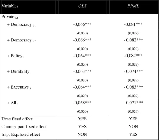
I perform a wide range of sensitivity analyses to assess the robustness of the empirical results (see tables III, IV, V and VI). First, I consider a set of additional control variables to control for the independence of the relationship between financial development and the intensive margin of trade. More specifically, there is a vast body of literature showing that good policy and institutional environment promote better trade performance (see Levchenko, 2007). The correlation between these economic characteristics and financial development could therefore explain the previous results. I use two democratic development indicators, a political environment measurement, a political sustainability indicator and an indicator of the level of political authority and corruption. Data are available from Polity IV and the World Bank. None of the specifications tested changes

24

either the sign or the significance of the financial coefficient25.

The empirical results could also be influenced by a reverse causality bias. Income and credit in the economy may vary with exports, which would result in an endogenization of the financial indicator. To control for this bias, I use a 3-, 5- and 7-years moving average for the financial indicator. This procedure reduces the possibility of simultaneous adjustments between trade and finance. The results confirm the findings in Table II. The coefficients are negative with all three indicators in the linear and non-linear models.

I then check the influence of outliers. First, I examine the residuals from the linear regression. I remove all observations with a residual greater than three standard deviations from zero and I re-estimate the linear model. Then I remove the five countries that export the most and the least, and I re-estimate equation 18. The financial variable's coefficient is negative and significantly different from zero in both specifications tested.

I also select four different measurements of financial development to test whether the results are robust to the choice of indicator. The four variables selected are those the most often used by the literature: Bank, Financial Depth, Capitalization and Liquidity26. The first measures the ratio of bank deposits to total deposits. Financial Depth measures total financial intermediation as a percentage of GDP. The last two variables measure stock market development: Capitalization equals the ratio of market capitalization to GDP while Liquidity measures market liquidity. Despite the robustness of the results using Private, in general, these four indicators' coefficients are not significantly different from zero. The only exception is Liquidity, whose coefficients are negative and significant at 1% in both linear and non-linear models. However, the sign and significance of the other variables are inconstant and depend on the model estimated.

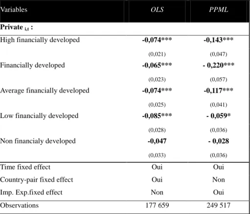
Lastly, I test the linearity of the financial effects on exports. I separate the 135 countries into five sub-groups by their stage of financial development and I create a dummy for each group. I then interact these variables with Private. Both linear and non-linear model estimates using the dummies find negative coefficients for the five sub-groups. This suggests that the results are not influenced by a specific country category. However, the least developed group has a insignificant coefficient in both models, indicating that financial improvements at this development stage do not affect trade.

25 _{The estimate's first step remains the same for all robustness tests.} 26

Conclusions

This article explores the relationship between firms' financial constraints and the margins of international trade. It is part of a recent body of literature, to which it contributes in two main ways. First, the article examines the macroeconomic impact of the relationship, broadening the sector focus found elsewhere in the literature. Second, it provides new information about firms' exporting behavior under financial constraints.

The article constructs a theoretical model, which is tested by an empirical analysis, showing that the level of financial development is positively correlated with the proportion of exporting firms (the extensive margin). However, once the relationship is established, the volume of firms export is not affected by changes in financial constraints. Therefore, the theoretical model does not define a clear relationship between finance and trade flows (the intensive margin).

The empirical analysis draws on a panel database covering 135 countries between 1994 and 2007. I estimate a probit model to test the effect of finance on the extensive margin. The results confirm the theoretical proposition. I then estimate a two-step gravity equation to analyze the effects of finance on trade flows. The results are striking, turning up a negative relationship between financial development and the intensive margin.

The link between finance and trade channels through firm selection. When the financial constraints are relaxed, the productivity cut-off above which firms export is reduced and a greater proportion of firms can access foreign markets. In the other hand, the finance - intensive margin relationship follows two distinct paths. The literature differentiates the industries by their level of dependence on external finance and finds that financial development translates into a comparative advantage in financially vulnerable sectors. This article demonstrates, however, that the macroeconomic impact of financial development on exports, all industries together, was negative during the analyzed period.

Table I: Financial constraints and the extensive margin

Variables Tij,t (Probit RE) Tij,t (Probit PA) Tij,t (Logit FE)

Private i,t 0.207*** (0.013) 0.122*** (0.007) 0.059** (0.030) Distance ij -0.937*** (0.023) -0,549*** (0.012) GDP i,t 0.629*** (0.010) 0.352*** (0.006) -0.020 (0.048) GDP j,t 0.617*** (0.009) 0.348*** (0.005) 0.114** (0.048) Population i,t 0.100*** (0.013) 0.055*** (0.007) -1.710*** (0.194) Population j,t 0.019* (0.012) 0.016** (0.007) -1.648*** (0.191) FTA ij,t 0.410*** (0.069) 0.037 (0.032) 1.501*** (0.225) WTO ij,t 0.307*** (0.019) 0.192*** (0.010) 0.293*** (0.042) Currency ij,t 0.919*** (0.120) 0.699*** (0.074) 1.707*** (0.332) Contig ij -0.202 (0.156) -0.250*** (0.085) Langue ij 0.509*** (0.040) 0.277*** (0.022) Colony ij 2.149*** (0.490) 1.249*** (0.338) SameCtry ij 0.797*** (0.203) 0.305*** (0.109) Landlock ij -0.276*** (0.026) -0.178*** (0.014) Island ij 0.351*** (0.032) 0.232*** (0.018) Area i -0.014* (0.009) 0.001 (0.005) Area j -0.062*** (0.009) -0.030*** (0.005)

Time Fixed Effect YES YES YES

Observations 249 517 249 517 91 924

Table II: Financial constraints and the intensive margin

Variables xij,t OLS Xij,t PPML Polynomial (xij,t OLS) Polynomial (Xij,t PPML) Private i,t -0.070*** (0.019) -0.089*** (0.029) -0.070** (0.019) -0.093*** (0.029) Distance ij -0,768*** (0.010) -0,765*** (0.010) GDP i,t 0.244*** (0.033) 0.535*** (0.045) 0.246*** (0.033) 0.499*** (0.045) GDP j,t 0.563*** (0.031) 0.567*** (0.044) 0.564*** (0.031) 0.565*** (0.044) Population i,t -0.694*** (0.152) -0.287 (0.218) -0.671*** (0.152) -0.499** (0.221) Population j,t 0.625*** (0.139) -2.007*** (0.207) 0.616*** (0.139) -2.097*** (0.209) FTA ij,t 0.194*** (0.023) 0.374*** (0.019) 0.191*** (0.023) 0.376*** (0.019) WTO ij,t 0.321*** (0.027) 0.292*** (0.046) 0.320*** (0.027) 0.262*** (0.046) Currency ij,t 0.469*** (0.118) 0.009 (0.024) 0.464*** (0.118) 0.032 (0.024) Contig ij 0.437*** (0.019) 0.440*** (0.019) Langue ij 0.233*** (0.018) 0.232*** (0.018) Colony ij 0.003 (0.061) -0.000 (0.060) SameCtry ij 0.096* (0.051) 0.103** (0.051) W ij,t 0.020** (0.009) 0.078*** (0.013) λ(Z ij,t) 0.359*** (0.043) 4.737*** (1.501) Z ij,t 3.058*** (1.046) -0.044 (0.044) (Z ij,t) 2 -0.871*** (0.302) 0.021 (0.029) (Z ij,t) 3 0.082*** (0.029) 0.001 (0.004)

Time Fixed Effect YES YES YES YES

Country-pair Fixed Effect YES NO YES NO

Exp. Imp. Fixed Effect NO YES NO YES

Observations 177 659 249 517 177 659 249 517

Table III:The independence of financial indicator

Variables OLS PPML Private i,t : + Democracy i 1 -0,066*** -0,081*** (0,020) (0,029) + Democracy i 2 -0,066*** - 0,082*** _{(0,020) (0,029)} + Policy i -0,064*** -0,082*** (0,020) (0,029) + Durability i -0,063*** - 0,074*** (0,020) (0,029) + Executive i -0,064*** - 0,083*** _{(0,020) (0,029)} + All i -0,068*** - 0,071*** _{(0,020) (0,029)}

Time fixed effect YES YES

Country-pair fixed effect YES NON

Imp. Exp.fixed effect NON YES

*** indicates the coefficient significance level at 1%, ** at 5% and * at 10%

Table IV: 3- 5- and 7- years moving average

OLS PPML Private i : 3 years -0,110*** -0,098*** _{(0,023) (0,036)} Private i : 5 years -0,092*** -0,095** _{(0,030) (0,045)} Private i : 7 years -0,129*** -0,088* (0,043) (0,068)

Time fixed effect YES YES

Country-pair fixed effect YES NON

Imp. Exp.fixed effect NON YES

Table V: Different financial indicators

Variables OLS PPML

Bank i,t -0,063* 0,059

(0,038) (0,046)

Financial Depth i,t 0,014 0,096*

_{(0,029) (0,053)}

Capitalization i,t -0,002 0,067***

_{(0,011) (0,018)}

Liquidity i,t - 0,021*** -0,053***

(0,007) (0,013)

Time fixed effect YES YES

Country-pair fixed effect YES NON

Imp. Exp.fixed effect NON YES

*** indicates the coefficient significance level at 1%, ** at 5% and * at 10%

Table VI: The linearity of the financial effects on exports

Variables OLS PPML

Private i,t :

High financially developed -0,074*** -0,143***

(0,021) (0,047)

Financially developed -0,065*** - 0,220***

(0,023) (0,057)

Average financially developed -0,074*** -0,117***

_{(0,025) (0,041)}

Low financially developed -0,085*** - 0,059*

_{(0,028) (0,036)}

Non financialy developed -0,047 - 0,028

(0,033) (0,036)

Time fixed effect Oui Oui

Country-pair fixed effect Oui Non

Imp. Exp.fixed effect Non Oui

Observations 177 659 249 517