Competition, Innovation and Distance to Frontier

Documents de Travail du

Centre d’Economie de la Sorbonne

Maison des Sciences Économiques, 106-112 boulevard de L'Hôpital, 75647 Paris Cedex 13

Competition, Innovation and Distance to Frontier

Bruno AMABLE, Lilas DEMMOU, Ivan LEDEZMA

Competition, Innovation and Distance to

Frontier

Bruno Amable, Lilas Demmou

and Ivan Ledezma

July 2008

Abstract

According to a recent literature, the positive e¤ect of competition is supposed to be growing with the proximity to the technological fron-tier. Using a variety of indicators, the paper tests the e¤ect of com-petition and regulation on innovative activity measured by patenting. The sample consists of a panel of 15 industries for 17 OECD countries over the period 1979-2003. Results show no evidence of a positive e¤ect of competition growing with the proximity to the frontier. Two main con…gurations emerge. First, regulation has a positive e¤ect whatever the distance to the frontier and the magnitude of its impact is higher the closer the industry is to the frontier. Second, the e¤ect of regulation is negative far from the frontier and becomes positive (or non signi…cant) when the technology gap decreases. These results con-tradict the belief in the innovation-boosting e¤ect of product market deregulation such as taken into account in the Lisbon Strategy.

Keywords: Innovation, competition, distance to frontier JEL codes: O30, L16,

1

Introduction

Concerns about the lack of convergence of Europe’s productivity level vis-à-vis the US over the past decade have been expressed not only in academic circles but also among policy makers and politicians. As numerous reports have shown (Kok, 2004; Sapir, 2004), Europe seems to be losing ground,

University of Paris I Panthéon - Sorbonne & CEPREMAP

y_{DGTPE, Ministry of Finance}

not because of an insu¢ cient rate of capital accumulation, but for lack of innovation capability. The so-called Lisbon Strategy, which aims at foster-ing innovation and productivity, proposes a series of structural reforms for labour, …nancial and product markets. Regarding the latter, a link between competition and innovation underlies the whole Lisbon Strategy: more prod-uct market competition should bolster innovation and thus prodprod-uctivity and

growth.1

According to economic theory, the relation between competition and in-novation is ambiguous. For Schumpeter (1934), monopoly pro…ts are rewards to innovators; the appropriability of innovation output is thus a crucial incen-tive issue. A rise in competition is expected to decrease rents stemming from innovation and thus incentives to innovate. This traditional "Schumpeterian e¤ect" of competition is featured in numerous innovation-based endogenous growth models, in particular Aghion and Howitt (1992) where innovation e¤ort increases with the Lerner index.

On the other hand, competition may encourage innovation. Incumbents may innovate to keep their market power and fend o¤ new entrants, or po-tential entrants may hope to capture the market position of incumbents by surpassing them with new and better products. In both cases, innovation would be the means for a …rm to get the upper hand over its competitors. Extensions of the Schumpeterian innovation-based endogenous growth model allow to take into account di¤erentiated in‡uences of competition on innova-tion. The situation analysed in Aghion et al. (2005) is that of a competition between rivals with di¤erent productivity levels. Firms innovate to decrease their production costs "step by step": a technological laggard has to catch-up with the technological level of the leader before having the possibility of becoming itself a leader in the industry. The risks for the leader to lose its position are therefore increased when the competitor is only one step away from catching-up. When competitors have comparable productivity levels, i.e. the so-called "neck and neck" competition, a stronger competition will induce …rms to increase their innovative investments in order to acquire a competitive lead over rival …rms. This pro-innovation e¤ect of competi-tion is less prominent in industries where the leader has a marked advan-tage over its competitor. The incorporation of both innovation-inducing and innovation-deterring e¤ects of competition into a single model leads to a non-linear, inverted U-shaped, relation between product market competition and innovation (Aghion et al., 2005).

The link between competition and innovation has been investigated pri-marily at the …rm level. The possible existence of an e¤ect of the …rm’s size

or market power on its innovative activity is a well-known topic in the inno-vation literature (Baldwin and Scott, 1987; Cohen and Levin, 1989; Geroski, 1995). Although both pro- and anti-innovation e¤ects of competition may be found in the empirical literature, the recent contributions tend to establish contrasted results di¤erencing …rm size e¤ects from more general competi-tion in‡uences. Using a sample of French …rms, Crépon, Duguet and Kabla (1995) found that market power stimulates innovation, although this e¤ect seems to be small in magnitude. Crépon, Duguet and Mairesse (1998), in a four equation model for French manufacturing …rms taking into account the …rm’s decision to engage in R&D activities, the R&D intensity, the e¤ects of R&D on patenting and the e¤ects of patenting on productivity, con…rmed the existence of a size e¤ect in the decision to engage in R&D activity but not the R&D intensity. On the other hand, market share and diversi…cation a¤ect positively both the decision to undertake R&D and R&D intensity. Competition may also exert negative e¤ects such as those found in Crépon and Duguet (1997): competitors’ R&D may have a negative impact on a …rm’s own innovation e¤ort, indicating the existence of a rivalry externality that acts as a disincentive to innovate.

On the other hand, Nickell (1996) showed with a panel of 670 UK …rms that competition, measured by a high number of competitors or low levels of rents, is associated to high rates of TFP growth. Whether this reveals a direct e¤ect of competition on productivity, through a slack-reducing e¤ect for instance, or an indirect e¤ect through innovation is undecided. Blun-dell, Gri¢ th and vanReenen (1999) used a panel of 340 British manufac-turing …rms between 1972 and 1982 and showed that the relation between competition and innovation possesses contrasted features. Industries where concentration is higher and import penetration lower have fewer innovations. This …nding tends to support the existence of a positive relationship between competition and innovation. However, within industries, …rms with a higher market share tend to commercialise more innovations. They also showed that larger …rms produce innovations of a greater commercial value than smaller …rms.

The duality of competition’s e¤ects on innovation is summarised in the …ndings of Aghion (2003) and Aghion et al. (2005). With the help of …rm-level data and US Patent O¢ ce data quoted on the London Stock Exchange between 1968 and 1997, they presented evidence of an inverted U-shaped relationship between the Lerner index and the number of patents granted. The "Schumpeterian e¤ect" of competition should dominate when the level of competition is high whereas the "escape competition" e¤ect should be prominent at low levels of product market competition. Moreover, following the prediction of the theoretical model, the inverted U-shaped relationship

was found to be steeper for …rms that are closer to the leading edge in their industry.

Empirical evidence at the industry level is far less abundant than at the …rm level. Industry-level studies have the advantage of allowing to escape from the limits of the proxies for competition usually taken into account by micro-level studies such as …rm size, market power or pro…tability level, and consider actual industry-speci…c or macroeconomy-wide competition policy measures. Gri¢ th, Harrison and Simpson (2006) measured innovation by Business Entreprise R&D expenditure for 12 industries and nine countries over the 1987-2000 period and investigated the e¤ect of the Single Market Programme. Using a dummy variable for the post-SMP years, they found that the SMP had a positive impact on innovative activity in a¤ected in-dustries and countries. They interpreted their results as a support for the competition-enhancing reforms advocated within the Lisbon Agenda. Nico-letti and Scarpetta (2003) considered a sample of 23 industries for 18 OECD countries over the period 1984-1998. They tested a model of TFP growth using product market regulation indicators devised by the OECD both alone and in interaction with a technology gap variable. They found statistically signi…cant positive coe¢ cients on the interacted variables, a result they in-terpreted as a catch-up slowing-down e¤ect of product market regulation. Conway et al. (2006) tested a similar model of labour productivity with interaction terms between product market regulation indicators and a tech-nology gap measure on a slightly extended sample of OECD countries. They found a signi…cantly positive coe¢ cient on the interacted variables too, which they interpreted as a catch-up slowing-down e¤ect.

The di¤erentiated e¤ect of product market competition according to the distance to the technological frontier is a central issue of the whole compe-tition and innovation debate. The received argument is that the economic costs of product market regulation increase the closer an economy is to the technological frontier (Aghion, 2006). For Aghion et al. (2006), increased competition, represented by a higher entry threat, spurs innovation incentives in sectors close to the technological frontier, whereas it discourages innova-tion in laggard sectors through a tradiinnova-tional Schumpeterian rent-diminishing e¤ect. Testing a model of TFP growth and a model of innovation (patent-ing) with foreign entry and distance to the technological frontier variables included both alone and interacted along with other competition variables on micro-level data for the UK, they concluded that, as an economy moves closer to the technological frontier, the competitiveness of all industries in a high-cost high-productivity economy depends on the ability to innovate. This applies to all sectors of the economy, "high-tech" or not, since the R&D intensity of all industries increases when economies move closer to the

tech-nological frontier (Acemoglu, Aghion and Zilibotti, 2006).

Concerning the inverted U-shape pattern, Tingvall and Poldahl (2006) …nd that, for Sweden …rms, the support for this pattern depends on the in-dicator. While the Her…ndal- index gives support to the inverted U-shape, the price cost margin does not allow to …t this pattern. Moreover, the use of time-series estimators reduces considerably the signi…cance of results. Aske-nazy, Cahn and Irac (2007), using a panel of French …rms, …nd that the concavity of the courbe linking competition and innovation is substantially reduced when the size of …rms is small relatively to the cost of innovation. For the authors, this type of …rms represents 85% of the sample.

The aim of this paper is to assess the validity of the argument according to which competition spurs innovation, and that this e¤ect is all the more important that an economy is close to the technological frontier. A dynamic model including variables for the distance to the frontier, competition, as well an interaction term between them is estimated. The empirical strategy of this paper di¤ers from the existing academic literature on three levels. First, the analysis is conducted at the industry level, while most empirical evidence focuses on micro studies. To the best of our knowledge, this is the …rst work testing the impact of competition on innovation at the industry level with a cross-country panel. Second, we use not only indicators for observed mea-sures of competition but also indicators of regulation policy (institutional indicators, and output measure of competition). Finally, we run regressions using di¤erent estimators (OLS, …xed e¤ects and system GMM) in order to take into account the dynamic nature of the innovative process and propose di¤erent extensions of the baseline model. The use of di¤erent variants of the model, di¤erent estimators and di¤erent indicators to measure the intensity of competition helps to assess the robustness of our …ndings. The evidence does not give support to an innovation-bolstering e¤ect of product market competition at the technological frontier. Moreover, the marginal e¤ect of regulation, conditional on the closeness to the technological frontier, tends to be upward sloping, meaning that regulation might indeed foster innovation at the leading edge. The measure of observed competition (relative number of …rms) presents a positive e¤ect only for laggard industries and it vanishes close to technological frontier. These results along with previous micro evi-dence, suggest that deregulation policiy does not seem to be a substitute for active science and technology policies, which do present a signi…cant impact on technical change (Guellec and de la Potterie, 2003)

The paper is organised as follows. Section 2 presents the empirical strat-egy and the problems related with the estimations. Section 3 intrioduces the data used in the empirical analysis. The following Section presents the results of the baseline model. Section 5 proposes extensions and robustness tests of

this model. Section 6 discusses the theoretical argument relating innovation with competition and sheds light on a possible explanation of our results: the inclusion of innovative leaders into the Aghion et al.’s (2005) model makes the relationship between the innovation-fostering e¤ect of competition and distance to frontier more complex. A brief conclusion follows.

2

Empirical strategy

2.1

Dynamic issues

Our purpose is to test the impact of competition on innovation with a

time-series-cross-section data at the industry level for OECD countries. This

structure has two particularities. First, information on innovation is ag-gregated and belongs to individuals which represent di¤erent activities per-formed in di¤erent countries. Second, a plausible model of the innovation process should exploit this panel structure and allow for a dynamics in which past innovations help to explain current ones. These particularities imply a non-negligible unobserved heterogeneity among individuals that will be

present in both past and current innovation. More speci…cally let pit be our

proxy of innovation activity in natural log and summarise, for the moment,

our explanatory covariates (in log) on the vector xit. Our problem can be

formulated as the estimation of the following dynamic multivariate model:

pit = pit 1+ xit+ it (1)

Where it= i+ it

The main issue is that the past realisation of our dependent variable is endogenous to the …xed e¤ect in the error term. In this framework, the

estimates of provided by OLS are upward biased and those coming from the

Within-group estimator are downward biased (Bond 2002; Benavente et al. 2005). While the former neglects the unobserved time-invariant heterogeneity

i, which is the source of correlation between pit 1and it, the latter includes

past values of pit since it subtracts the mean to eliminate i. Although these

estimators are biased, they are useful because they give an interval in which

a consistent estimation of should lie.

Several strategies can be adopted to face these dynamic concerns. They go

from the estimation of the model in di¤erences, by instrumenting pit 1with

pit 2 using a two stage least squares (Andersen and Hsiao, 1981), to di¤erent

techniques based on the generalised method of moments (GMM). GMM-based methods improve e¢ ciency by exploiting the moment conditions that relate deeper lags of the dependent variable, some times transformed, to the

error term. Among GMM techniques we are particularly interested in the one suggested by Arellano and Bover (1995) and fully developed by Blundell and Bond (1998), usually called system GMM (S-GMM). The di¤erence GMM (D-GMM) proposed by Arellano and Bond (1991), which applies a transfor-mation in di¤erences and uses the orthogonality conditions of available lags

of pit 1, is augmented by S-GMM under the assumption that …rst di¤erences

of the instrumenting variables are uncorrelated to the error in levels. Thanks to this assumption, one can include the original equation in levels and use

pit 2 and deeper as instruments for pit 1. The transformed equation and

the one in levels make a system in which more instruments can be exploited. The use of a new set of instruments in di¤erences improves e¢ ciency as it deals with the problem of weak instruments of D-GMM in persistent series.

Note that equation (1) is equivalent to state pit = ( 1) pit 1+ xit+ it.

Hence pitis weakly correlated with pit 1 if is close to 1. Intuitively, in the

case of a process close to a random walk, past values will not predict current changes as good as past changes can predict current values. In that sense,

one can expect that instrumenting pit 1 with pit s (s = 2::T ) should give

more accurate estimates. On the other hand, the inclusion of the equation in levels will be useful to keep the information of variables that do not change too much during time. This is namely the case of our proxies of regulation.

It should be stressed that our measure of innovation is based on the ag-gregation of patents at the country level and distributed at the industry level according to a transformation matrix linking technology and industry clas-si…cation. In addition, to take into account …xed e¤ects related to size and economic activity we normalize this measure dividing by the hours worked. In this context, it seems reasonably to treat this aggregated normalised mea-sure of innovation as a continuous variable rather than counts coming from independent experiments.

2.2

Specifying regressors

x

One advantage of GMM techniques is that they allow the other regressors

xit to be predetermined (explained by their past realisations) or endogenous

(explained by current and past realisations of other variables and by their own autoregressive process). In our basic estimation, we consider as explanatory

variables xitthe closeness to the frontier clit, the product market competition

proxy mcit and their interaction mcit clit. As elemental controls we also

include in all regressions the capital intensity klit and the externalities exit

arising from the innovative activity of the same industry in the rest of the world. The interaction term will capture the extent to which product market competition in‡uences the innovative process conditional to the proximity to

the technological frontier. We also include year dummies dtin order to control

for macroeconomic shocks homogeneous across individuals. The following baseline model is estimated:

pit = pit 1+ 1clit+ 2 mcit clit+ 3mcit+ 4 klit+ 5 exit+ 6 dt+ it (2)

Even though the S-GMM estimator deal with the potential endogeneity of the regressors, as a robustness check, to reduce the risk of reverse causality, we also estimate the model considering the explicative variables lagged once:

pit = pit 1+ 1clit 1+ 2mcit 1 clit 1+ 3mcit 1+ 4klit 1+ 5exit 1+ 6dt+ it

(3) Aiming at getting further insights about the concavity of the e¤ect of competition, we augment the reduced form of the interaction and include the squares terms of the closeness to the frontier and product market com-petition:

pit = pit 1+ 1clit+ 2mcit clit+ 3mcit+ 4klit+ 5exit+ 7cl2it+ 8mc2it+ 6dt+ it

(4) This speci…cation is equivalent to consider a translog approximation of a constant elasticity function between both variables that can be more precise to capture an eventual complementarity between them. A similar equation is also estimated for the model with all regressor in lag 1. Finally, we test an extended version of (2) and (4), including further controls such as import penetration, …nancial deepness and labour market regulation.

In all S-GMM regressions the set of instruments is composed of the

de-pendent variable pit, the closeness to the frontier clit, the product market

competition mcit; and their interaction mcit clit, all in lag two or deeper.

We also use as instrument the externalities exit in lag 1 (or deeper) as we can

exploit its expected exogeneity. Since the Sargan-Hansen test for overiden-tifying restriction, which tests the exogeneity of instruments, becomes less rigorous as the number of instruments increases, the recommendation is to have less instruments than individuals (Roodman, 2006), a rule that is in line with evidence provided by simulation (see Windmeijer 2005). Since the number of instrument is quadratic in time dimension and S-GMM generates not only a set of instrument for the transformed equation but also for the equation in levels, this rule, for our sample size, is some what constrain-ing. We overcome this di¢ culty by using limited lags, by considering most

informative instruments and by collapsing in some cases the matrix of an in-strumenting variable into a vector. The latter strategy is equivalent to sum up independent moment conditions in one equation. Examples of this strat-egy are Calderon et al. (2002) or Beck and Levine (2004). In each case, the main criterion to accept the instrumentation strategy is the Sargan-Hansen test and its version in di¤erence which allows to test a subset of instruments. In addition, we pay special attention to the autocorrelation of the error term, a crucial assumption for the validity of instruments in lag 2. To do so, use is made of the Arellano-Bond test for serial correlation in di¤erences. Since by construction …rst order correlation is expected we only focus on the test

for second order correlation in di¤erence, which relates it 1 with it 2 by

looking at the correlation between it and it 2.

2.3

The marginal e¤ect of competition on innovation

Since we have included an interaction term between product market

compe-tition and the closeness to technological frontier (mcit clit), the assessment

concerning the expected overall e¤ect of product market competition mcit

needs the computation of its marginal e¤ect conditional on speci…c values of

the closeness to technological frontier clit (Braumoeller 2004):

@E(pit=xit)

@mcit

= b₂clit+ b3 (5)

For the translog version: @E(pit=xit)

@mcit

= b₂clit+ b3+ 2b8mcit (6)

Similar expressions hold for (3) and the lagged version of (4). It is easy to

see, for instance, that a positive and signi…cant b₂ means nothing but that

competition increases innovation activity only for an individual completely

far away the technological frontier (clit = 0). That is for the unrealistic

case of zero labour productivity. Notice that for the augmented version (4), the calculation of the marginal e¤ect of competition depends on the level of

competition itself mcit in (6):

As each of these linear combinations is computed using the estimated

values of 2, 3 and 8; one still needs to determine their signi…cance, which

in turn will depend on the variance of estimates and the value at which clit

is evaluated (Friedrich 1982). For the (5), this signi…cance is given by the ratio

b₂clit+ b3

q

bb₃b₃ + cl2itbb₂b₂ + 2clit2bb₂b₃

Where_{b is the sample covariance between and . Hence, statistically}

insigni…cant coe¢ cients may combine to produce statistically signi…cant con-ditional e¤ects. In our regression we evaluate the marginal e¤ect and its signi…cance for the minimum, one deviation under the mean, the mean, one

deviation over the mean and the maximum sample values of clit. For the

translog version we take the mean value of mcit:

2.4

Testing for unit root

The validity of lagged di¤erences as instruments for levels depends on whether this lagged di¤erences are uncorrelated with the error term. Blundell and Bond (1998) state this assumption in terms of the stationarity of the initial conditions of the autoregressive process. Let us consider the reduced AR(1) version of our model:

pit = pit 1+ it it = i+ it (7)

If the initial conditions do not deviate systematically from their long

term stationary value E yi1 ₁ i i = 0; it follows that the deviation

itself will be uncorrelated with the …xed e¤ect. Thus, for the second period onwards the di¤erence of the dependent variable will be also uncorrelated with the …xed e¤ect. In other words, under this assumption, a …rst di¤erence

transformation of the instrument will be enough to purge _i. If there is no

serial correlation of it, then E [ pit 1 it] = 0.

As a consequence, we verify the risk of unit root of our main time series variables by the means of the Fisher test developed by Maddala and Wu (1999) for panel data. Alternative tests such as Levin, Lin and Chu (2002) and Im, Pesaran and Shin (2003) seem less convenient for our case. First, Levin, Lin and Chu (2002) consider the strong assumption that all units have the same autoregressive coe¢ cient. This assumption constraints the alternative hypothesis to posit that all series are stationary. Second, the single statistic of the Fisher test, resuming the signi…cance of all individual

unit root test, has an exact 2_{distribution. On the contrary, Im, Pesaran and}

Shin (2003) consider the mean of the t-statistic of each Augmented Dickey-Fuller individual test, whose normality is asymptotic. Finally, as both tests assume that the sample period is the same for all cross-section units, they need a balanced panel data. This reduces the size of the sample and the e¢ ciency of the test.

Results of these tests are reported in Table 13 (appendix). In order to allows for serial correlation in the error term we consider one and two

lags of yit for each individual Augmented Dickey-Fuller test. We do not

take a risk rejecting the null hypothesis of non stationary for all series when the autoregressive model considers a constant (drift). This speci…cation is consistent with our regressions.

3

Data

We collected information for 17 OECD countries and 15 manufacturing in-dustries at two-digit ISIC-Rev3 from 1979 to 2003 (Table 8). Original data

come from OECD-STAN, GGDC-ICOP project2_{and EUROSTAT databases.}

From OECD-STAN we use trade indicators and investment series. Starting from OECD-STAN, the GGDC-ICOP data complete the information with

surveys and their own estimations, consistent with national accountings.3

This data is our original source for value added series, implicit de‡ators and hours worked. Patent series were obtained from EUROSTAT, which dis-tribute by industries the number of patents granted according to a matrix relating technology and industry classi…cation.

3.1

Distance to frontier

Labour productivity (value added per hour worked) is used as the main mea-sure of e¢ ciency. The technological frontier is de…ned as the most productive available technology for each ISIC-Rev3 Industry at every period. The indi-vidual (country-industry couple) having the maximum labour productivity among all countries in a given year is identi…ed as the technological leader for that year. The closeness to the frontier is measured as the ratio of labour

productivity relative to that of the frontier.4 _{For instance, the closeness to}

the frontier of Spain in chemical industry in 1994 is the labour productivity

2_{The International Comparisons of Output and Productivity (ICOP) project of the}

Groningen Growth & Development Centre (GGDC)

3_{GGDC-ICOP estimate OECD-STAN missing information going to alternative sources}

and applying di¤erent estimation methods. However, the resulting dispersion is consider-ably bigger (See GGDC rows in Table 3.9 in appendix). We drop GGDC-ICOP estimations of industry 30 (o¢ ce machinery) because of its high dispersion and keep the OECD-STAN values for GGDC-ICOP outliers when OECD information exists. The global dispersion considerably diminishes (Filtered Data). With this …lter we get 6098 observation instead of 4129, with series quite comparable to those available in OECD-STAN.

of the Spanish chemical industry in 1994 divided by the highest labour pro-ductivity level for chemicals among all countries in that year. We consider a moving average of three year in order to smooth the series.

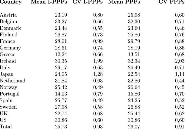
All nominal series were de‡ated to 1997 in their national currency. How-ever, in order to make an international comparison at the industry level, we need to take into account price di¤erences among countries at the industry level (cross section de‡ation). This is particularly important for value added series since we base our productive measure on them. Use is made of the in-dustry purchasing power parities (I-PPPs) provided by Timmer, Ympa and van Ark (2006) for 1997. The authors consider a mix between purchasing power parities based on two points of the productive process: consumer ex-penditure and production. Exex-penditure PPPs are computed from ICP index and production PPPs from average producer prices, which are calculated at the industry level dividing output values by quantities. While the former in-cludes only …nal goods and must be adjusted for taxes, distribution margins and trade costs, the latter needs to face the problem of matching varieties of goods that may di¤er in quality and product de…nition among countries. The selected PPPs measure (adjusted-expenditure or production) depends on the speci…city of each industry. The authors propose a harmonised dataset of purchasing power parities disaggregated at the industry level (I-PPPs) for a wide sample of developing countries. Aiming at getting comparable series, they apply the multilateral weighted aggregation method proposed by Elteto and Koves (1964) and Szulc (1964) (EKS). This method allows to obtain transitivity in multilateral comparisons starting from binary comparisons.

Table 10 (appendix) shows the average labour productivity of each coun-try for the full sample period and compares the values whether one uses the standard (non-adjusted) expenditure PPPs at the country level or the industry-PPP computed by Timmer, Ympa and van Ark (2006). Table 11 (appendix) presents similar …gures at the industry level (world sample av-erage). At the country level the average of labour productivity for the full sample period seems similar among countries. However, the variation in-duced by both measures increases if one considers the industry level. This issue is important because the hierarchy in terms of productivity and namely the identi…cation of the frontier level might change.

3.2

Innovation

As a proxy of innovation we consider the number of patents. At the industry level, they are provided by EUROSTAT. In this database the applications at the European Patents O¢ ce (EPO) are linked to industry standard classi…-cations by the means of a detailed matrix of weights. This matrix builds on

…rm data allowing to relate ISIC industries to the subclasses of International Patent Classi…cation (IPC) categories. The US counterpart of the EPO is the United States Patents and Trademarked O¢ ce (USPTO). Both series are not directly comparable since the EPO system informs about applica-tions and the USPTO about patent granted. We consider the EPO system as it is more representative for the countries present in our sample. Aiming at controlling for market size e¤ects, patents are normalised by the hours worked of the industry. At the end we get a continuous aggregated measure of innovation that enables international comparisons at the industry level.

Information on R&D expenditure, disaggregated at the industry level, is available from the OECD ANDBERD database. Nevertheless, the intersec-tion between R&D informaintersec-tion and the availability of the rest of variables leads to a signi…cant reduction of the number of observations (mainly Aus-tria, Greece, Ireland and Portugal) and R&D data is only available from 1987.

3.3

Competition and regulation measures

Five indicators have been selected to capture product market competition. On order to capture the extent of competition, we use both input (de jure) and output (de facto) measures of the competitive environment. Within the …rst group of proxies, we consider four indicators of market regulation: (1) the global product market regulation PMR provided by the OECD and doc-umented by Conway, Janod and Nicoletti (2005); (2) the size of the public enterprise sector PMR(public), a component of PMR that focuses on state control; (3) the regulatory provisions in non-manufacturing sectors (tele-coms, electricity, gas, post, rail, air passenger transport, and road freight) summarised by the REGREF indicator, also provided by the OECD (Conway and Nicoletti, 2006) and (4) the corresponding e¤ect of these regulatory pro-visions on the manufacturing sector given by the REGIMP indicator, which is also documented by (Conway and Nicoletti, 2006). REGIMP is based on an input/output matrix de…ning the use of non-manufacturing sectors as in-puts in manufacturing. Thus, it aims at capturing the "knock-on" e¤et of regulation in selected non-manufacturing sectors on manufacturing.

On the other hand, we also consider a measure of the outcome of compe-tition, namelly the number of …rms per value added (N-FIRMS/VA), which is a proxy of market atomicity (or the inverse of the average size), usually expected to be the result of the reduction of market barriers.

The scope of these indicators is as follow. REGIMP and N-FIRMS/VA are consistent with our time-series-cross-section data structure. REGREF is a time series at the country level re‡ecting the evolution of the economy-wide

competitive environment. Finally, PMR and PMR(public) are computed at the country level for two point times (1998 and 2003). They have been distributed for two periods: before and after 2000. Since PMR is based on a collection of private and governmental practices, this distribution should be in line with the evolution of European market reforms. Figure 1 gives a picture of the hierarchy of countries depending on their regulatory environments.

Norway Italy Portugal Spain Austria Greece France Belgium Germany Ireland Japan UK Finland Denmark Netherla Sweden US .08 .1 .12 .14 .16 .18 country

Means of REGIMP, REGIMP

Greece Italy France Portugal Ireland Belgium Netherla Denmark Austria Spain Norway Finland Germany Japan Sweden UK US 2 3 4 5 6 country

Means of REGREF, REGREF

Italy France Spain Portugal Finland Belgium Germany Norway Japan Austria Netherla Sweden Ireland Denmark US UK 1 1 .5 2 2 .5 3 country Means of PMR, PMR Norway Greece France Austria Italy Finland Germany Belgium Ireland Netherla Sweden Spain Portugal Denmark UK US Japan 0 1 2 3 4 5 country

Means of PMR_Public, PMR(Public)

Figure 1. Hierarchy of regulatory environments

3.4

Controls

We use two elemental controls: capital intensity and innovation spillovers. Capital series were constructed using investment series and the standard Perpetual Inventory Method (PIM). This method uses the dynamic rule by which current capital stock equals the stock of the preceding period after depreciation plus current investment. To compute the initial stock, the PIM method supposes that pre-sample investment grows at a constant rate. Under the assumption of steady state this rate equals the one of value added. After applying this result to the dynamic rule, the initial stock becomes a function of initial investment, the global depreciation rate and the steady state growth rate of value added. We proxy the latter with the mean of the sample period and use a depreciation rate of 7.5%, the standard assumption. To capture

innovation spillovers, we consider patenting activity of the rest of the world in the same manufacturing industry (the number of patents per hour worked produced by the same industry in the rest of the world).

As additional controls, we also include indicators of foreign competition, labour market regulation and …nancial deepness: the import penetration ratio MPEN available in OECD-STAN at the industry level, the employ-ment protection indicator EPLBLD proposed by Amable, Demmou and Gatti (2007) at the country level, which updates the EPL indicator of the OECD, and the …nancialisation ratio de…ned as the total assets of institutional in-vestors relative to GDP. Table 12 (appendix) summarises the main descrip-tive statistics.

4

Results

4.1

OLS and Within-group regressions

Table 1 presents OLS and Within-group estimates of the e¤ects of competi-tion on patenting using de facto and de jure measures of competicompeti-tion: the number of …rms relative to value added (N-FIRMS/VA in columns [1] to [3]) the "knock-on" e¤ect of regulation in non-manufacturing sectors (REGIMP in columns [4] to [6]), the indicator of competition in non-manufacturing sec-tors (REGREF in columns [7] to [9]), the economy-wide indicator of product market regulation (PMR in [10] to [12]) and the indicator for public sector (PMR(Public) in [13] to [16]). The models di¤er with the inclusion of the lagged dependent variable and the estimator: OLS or Within-group panel estimator. Models [3], [6], [9], [12] and [15] are …rst di¤erence equations with no lagged dependent variable. This amounts to forcing the coe¢ cient of the lagged dependent variable in level to be equal to one.

As expected, the coe¢ cient on the lagged dependent variable di¤ers greatly between the OLS and …xed-e¤ect estimator, being greater for the former model. Also the signs of the coe¢ cients for the externality e¤ect and the capital/labour ratio are mostly signi…cantly positive. For each regres-sion, the lower panel of the Table presents the estimated marginal e¤ects of the competition indicator for di¤erent levels of the relative productivity level (the closeness to the frontier). The …rst line of the lower panel gives the value of the marginal e¤ect when the relative technological level is at its minimum (min), i.e. when the distance to frontier is at its maximum. The last lines give the marginal e¤ects and standard errors when the relative productivity level is at the maximum of the sample, i.e. at the technology frontier. Marginal e¤ects coe¢ cients are also presented for the mean value of

the relative technological level, the mean value minus one standard deviation and plus one standard deviation. Therefore, reading a column of the lower panel of the Table shows how the marginal e¤ect of competition changes as the distance to the technological frontier decreases and vanishes.

The interpretation of the marginal e¤ect for regressions [1] to [3], with the relative number of …rms indicator, di¤ers from the interpretation for the other indicators. A higher relative number of …rms is a direct measure com-petition since it informs about the number of competitors that share the same market. It can also be interpreted as an inverse measure of the average …rms’ size in the industry, related to the level of concentration in the industry. If competition is more favourable to innovation near the technological frontier, the marginal e¤ects should increase as the relative technological level aug-ments from its minimum to its maximum. Indeed, if one follows strictly the predictions of Aghion et al. (2005), Aghion (2006), one should expect a neg-ative marginal e¤ect of competition far from the technological frontier (the Schumpeterian e¤ect) and a positive e¤ect close to the frontier (the ’escape competition’e¤ect). Results reported in Table 1 show that, while the relative number of …rms is positively correlated with innovation in laggard industries, its e¤ect decreases as the industry moves closer to the technological frontier. At the leading edge the e¤ect of competition given by this indicator loses its signi…cancy. Having a less concentrated industry seems to matter more when the industry is far from the leading edge than when it is near. This result is true whatever the estimator or speci…cation, only the magnitude of the e¤ects and their signi…cance change. This result could be compared with the positive size e¤ect found in many micro studies of innovation. If the …rm size is a positive in‡uence on innovation, one may suppose that it will be all the more important that the technological competition is …erce, i.e. that the industry is close to the leading edge.

Using a proxy for size or concentration in the industry is subject to the usual limitations: it measures the outcome of the competition process, not so much the competitive environment. In this respect, the use of indicators of regulation will make it possible to avoid ambiguous interpretations of the results. The interpretation of the marginal e¤ects of regulation according to the proximity to thefrontier is straightforward. Again, if competition is good for innovation, product market regulation should exert a negative in-‡uence on patenting, all the more so that the distance to frontier diminishes. Indeed, for Conway, Janod and Nicoletti (2005) and Conwayand Nicoletti (2006), these regulation proxies re‡ect ant-competitive market barriers. Fol-lowing Aghion et al.’s (2005) predictions, regulation could be good when the industry is far from the frontier, but should gradually become detrimental as the distance to frontier is reduced. One observes contrasted results in

regres-[1] [2] [3] [4] [5] [6] [7] [8] [9] [10] [11] [12] [13] [14] [15] Patenting (t-1) 0.974*** 0.328*** 0.961*** 0.557*** 0.960*** 0.599*** 0.961*** 0.637*** 0.944*** 0.596*** (0.009) (0.072) (0.006) (0.032) (0.006) (0.029) (0.007) (0.029) (0.007) (0.030) Closeness to Frontier -0.030 -0.096* 0.003 0.026 -0.181 -0.077 -0.021 -0.001 0.062 0.001 0.013 0.068* 0.028 0.082** 0.027 (0.027) (0.056) (0.054) (0.089) (0.161) (0.151) (0.042) (0.045) (0.048) (0.029) (0.038) (0.038) (0.038) (0.039) (0.043)

Closeness × Competition (Regulation)

-0.010 -0.089 *** -0.006 0.012 -0.075 -0.043 0.023 -0.011 -0.047 -0.027 -0.069 -0.131* -0.007 -0.084 *** -0.013 (0.016) (0.028) (0.026) (0.042) (0.078) (0.069) (0.034) (0.041) (0.047) (0.052) (0.071) (0.079) (0.030) (0.032) (0.037) Competition (Regulation) 0.059 0.402*** 0.060 -0.024 -0.514 0.568* -0.026 -0.138 0.187 0.228 0.322 1.070*** 0.114 0.064 0.573* (0.065) (0.117) (0.107) (0.174) (0.348) (0.312) (0.142) (0.189) (0.219) (0.220) (0.341) (0.358) (0.125) (0.285) (0.333) Ex ternalities 0.032*** 0.330*** -0.066 0.039*** 0.419*** -0.021 0.041*** 0.351*** 0.005 0.038*** 0.306*** 0.013 0.057*** 0.327*** 0.011 (0.009) (0.088) (0.100) (0.006) (0.065) (0.062) (0.006) (0.061) (0.062) (0.007) (0.059) (0.059) (0.007) (0.060) (0.061) Capital Intensity 0.011 0.537*** 0.103 0.002 0.254*** 0.087** 0.002 0.246*** 0.082** 0.000 0.233*** 0.082** 0.004 0.249*** 0.081** (0.011) (0.083) (0.072) (0.009) (0.031) (0.036) (0.009) (0.031) (0.036) (0.009) (0.031) (0.036) (0.009) (0.031) (0.035) Y ear dummies Y es Y es Y es Y es Y es Y es Y es Y es Y es Y es Y es Y es Y es Y es Y es Number of O bs 1352 1352 1352 2646 2646 2646 2646 2646 2646 2521 2521 2521 2646 2646 2646 Individuals 133 133 148 148 148 148 134 134 148 148 Estimator OLS W ithin W ithin OLS W ithin W ithin OLS W ithin W ithin OLS W ithin W ithin OLS W ithin W ithin Closeness (sampl e valu es) [1] [2] [3] [4] [5] [6] [7] [8] [9] [10] [11] [12] [13] [14] [15] M inimum 0.039 0.233*** 0.048 -0.001 -0.655 *** 0.487** 0.016 -0.158 0.099 0.176 0.190 0.820*** 0.101 -0.094 0.549* (0.035) (0.064) (0.059) (0.095) (0.219) (0.195) (0.078) (0.116) (0.134) (0.123) (0.224) (0.226) (0.069) (0.245) (0.280) M

ean less one standard deviation

0.021** 0.080*** 0.037** 0.019 -0.781 *** 0.415*** 0.054** -0.177 *** 0.020 0.127*** 0.066 0.586*** 0.089*** -0.236 0.527** (0.010) (0.019) (0.018) (0.028) (0.137) (0.118) (0.026) (0.061) (0.068) (0.037) (0.145) (0.140) (0.020) (0.216) (0.240) M ean 0.017*** 0.043*** 0.035*** 0.025 -0.815 *** 0.395*** 0.065*** -0.182 *** -0.001 0.117*** 0.039 0.535*** 0.086*** -0.274 0.522** (0.006) (0.013) (0.012) (0.017) (0.130) (0.110) (0.018) (0.052) (0.057) (0.025) (0.138) (0.135) (0.010) (0.211) (0.231) M

ean plus one standard deviation

0.013* 0.006 0.032** 0.030 -0.849 *** 0.376*** 0.075*** -0.187 *** -0.022 0.106*** 0.013 0.485*** 0.083*** -0.312 0.516** (0.007) (0.016) (0.015) (0.022) (0.133) (0.110) (0.022) (0.049) (0.052) (0.027) (0.135) (0.136) (0.014) (0.206) (0.222) M ax imum 0.011 -0.008 0.031* 0.032 -0.859 *** 0.370*** 0.078*** -0.188 *** -0.028 0.102*** 0.002 0.465*** 0.082*** -0.323 0.514** (0.009) (0.019) (0.017) (0.026) (0.136) (0.112) (0.025) (0.049) (0.052) (0.031) (0.136) (0.138) (0.017) (0.204) (0.220) Note: Hu bert-W

hite corrected standard error

s in parentheses * p<0.10, * * p<0.05, * ** p<0 .01; All v ariables in log N-FIRMS/VA RE GI MP REGREF PMR PMR(Public) N-FIRMS/VA RE GI MP REGREF Dependent V ariable:

Patenting (patents decomposition /hours w

orked)

- OLS a

nd Within Gr

oup Estimators

Marginal Effect o

f Competition ([1] to [3]) and Reg

ulation ([4] to [15])

Regressions for Competition ([1]

to [3]) and R egulation ([4] to [15]) PMR PMR(Public) T a b le 1 .

sions using the REGIMP indicator (columns [4] to [6] in Table 1), which is provided in panel-data-like structure (times-series-cross-section data). The OLS regression gives marginal e¤ects non signi…cantly di¤erent from zero, i.e. no impact of product market regulation on innovation whatever the distance to frontier. The …xed e¤ect regression gives a statistically negative impact of regulation, which is increasing with the relative technological level. On the other hand, considering the model without the lagged dependent variable gives signi…cant positive marginal e¤ects of regulation.

Looking at the results documented in Table 1 (columns [4] to [15]), three con…gurations emerge. The most frequent case is that of a positive impact of regulation policy, which is decreasing as the industry approaches the tech-nological frontier but remains signi…cantly positive even at the frontier([6], [10],[12],[13] and [15]). In regression [7], this positive marginal e¤ect appears on the contrary to increase as the industry moves closer to the frontier. On the other hand, regulation policy turns out to have a negative signi…cant marginal e¤ect in regressions [5] and [8]. Although this e¤ect is decreasing with the closeness to the frontier, it appears signi…cantly negative for lag-gard industries. Furthermore, in some cases regulation turns out to have non signi…cant marginal e¤ects, no matter what the distance to the frontier is ([4],[9],[11] and [14]). Interestingly, even if these regressions do not allow to conclude to a single pattern of the relationship between competition and innovation, none of them reproduce the predictions of the baseline model.

4.2

Addressing dynamics (System-GMM regressions)

As argued in the previous Section, OLS and Within-group estimators may not be appropriate for the problem considered here. The use of the S-GMM estimator will allow us to deal with the lagged dependent variable bias and the potential endogeneity of several of the regressors. One may indeed sup-pose that the competition indicators taken into account here are endogenous. For instance, lagging …rms or industries may pressure for protection from competition in exchange for political support, whereas the support for regu-lation would be less pronounced in the vicinity of the technological frontier. Other variables may also be endogenous to the growth process itself. For these reasons, the competition indicators and the capital/labour ratio will be considered as endogenous in the S-GMM estimations.

N-FIRMS/VA REGIMP REGREF PMR PMR (Public) [1] [2] [3] [4] [5] Patenting (t-1) 0.896*** 0.903*** 0.843*** 0.922*** 0.887*** (0.064) (0.032) (0.049) (0.022) (0.033) Closeness to Frontier -0.013 1.924** -0.284 0.003 0.046 (0.126) (0.972) (0.230) (0.053) (0.129)

Closeness × Competition (Regulation) -0.113* 0.936** 0.494** 0.020 0.068

(0.067) (0.469) (0.198) (0.114) (0.096) Competition (Regulation) 0.509* -3.794** -1.926** 0.257 -0.144 (0.280) (1.909) (0.823) (0.450) (0.397) Externalities 0.177* 0.116** 0.219*** 0.084*** 0.114*** (0.105) (0.046) (0.064) (0.024) (0.036) Capital Intensity 0.032 -0.032 0.122 -0.041 0.118** (0.057) (0.041) (0.079) (0.039) (0.055)

Year dummies Yes Yes Yes Yes Yes

Number of Obs 1352 2646 2646 2521 2646

Sargan-Hansen p 0.387 0.164 0.117 0.187 0.224

AR(2)p 0.522 0.908 0.919 0.654 0.946

Instruments 122 136 131 106 142

Individuals 133 148 148 134 148

Estimator SY_GMM SY_GMM SY_GMM SY_GMM SY_GMM

N-FIRMS/VA REGIMP REGREF PMR PMR (Public)

Closeness (sample values) [1] [2] [3] [4] [5]

Minimum 0.294* -2.033** -0.997** 0.294 -0.017

(0.153) (1.027) (0.455) (0.264) (0.217)

Mean less one standard deviation 0.100** -0.451* -0.162 0.330* 0.098

(0.045) (0.240) (0.150) (0.175) (0.063)

Mean 0.053* -0.028 0.061 0.338* 0.128***

(0.028) (0.062) (0.105) (0.183) (0.038)

Mean plus one standard deviation 0.006 0.395** 0.284** 0.345* 0.159***

(0.035) (0.200) (0.125) (0.199) (0.052)

Maximum -0.012 0.516** 0.348** 0.348* 0.167***

(0.042) (0.258) (0.141) (0.208) (0.062)

Note: Hubert-White corrected standard errors in parentheses * p<0.10, ** p<0.05, *** p<0.01; All variables in log

Regressions for Competition ([1] ) and Regulation ([2] to [5])

Dependent Variable: Patenting (patents decomposition /hours worked) - System-GMM Estimations

Marginal effect of competition ([1]) and Regulation ([2] to [5])

0 .05 .1 .15 Hi sto gra m o f c lo sen ess -.2 0 .2 .4 .6 Margin al Effect

Minimum Mean Maximum

Closeness

firms/VA (SY_SGMM [1])

Figure 2. Marginal e¤ect of N-Firms/VA on patenting

Table 2 presents the S-GMM estimations of the e¤ects of competition on innovation. As in our previous results, the number of …rms plays a positive role for innovation, but only when industries are far from the technological frontier (Column [1]). This e¤ect vanishes once the relative productivity level rises above the mean. Figure 2 presents the plot of the marginal e¤ect against the closeness to the technological frontier. As one notices clearly with the con…dence intervals, a signi…cant innovation-boosting e¤ect exists only for industries under the mean relative productivity. The Figure displays also the histogram of the relative productivity levels. One notices that only a limited number of industry laggards are likely to bene…t from increased competition while the bulk of the industries would bene…t very little if anything.

0 .05 .1 Hi sto gra m o f c lo sen ess -4 -3 -2 -1 0 1 Margin al Effect

Minimum Mean Maximum

Closeness

reg_impact (SY_SGMM [1])

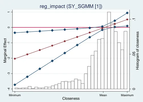
Figure 3. Marginal e¤ect of REGIMP on patenting

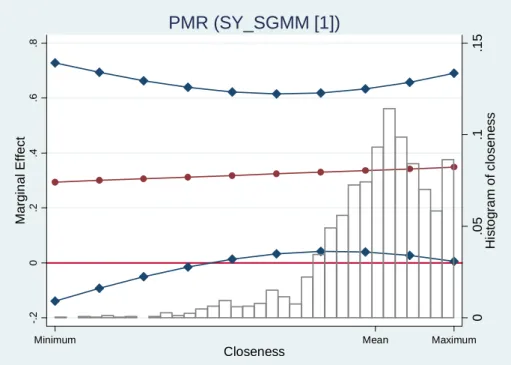
This e¤ect of competition is broadly con…rmed by the results obtained using the indicators of regulation. For the regulation impact (Column [2] and Figure 3) and regulation in non-manufacturing activities (Column [3] and Figure 4) indicators, competition regulation has a negative impact on innovation far from the frontier. This e¤ect becomes gradually positive as the relative productivity level increases above the mean and turns out to be signi…cantly positive at the frontier. The results for the economy-wide product market regulation indicators (Columns [4] and [5], Figures 5 and 6) are in line with those just mentioned. Product market regulation has no impact on innovation far from the frontier, and an increasingly positive e¤ect as the productivity level rises.

0 .05 .1 Hi sto gra m o f c lo sen ess -2 -1.5 -1 -.5 0 .5 Margin al Effect

Minimum Mean Maximum

Closeness

reg_services (SY_SGMM [1])

Figure 4. Marginal e¤ect of REGREF on patenting

On the whole, the use of an estimator well-suited to a dynamic speci…ca-tion allows to depict a clearer picture about the marginal e¤ect of competi-tion and regulacompeti-tion according to the proximity to the technological frontier: product market regulation has an increasingly positive impact on innova-tion as the industry moves closer to the frontier, i.e. the marginal e¤ects of regulation indicators display a positive slope. The …ndings with the relative number of …rms as a proxy for the outcome of market competition are consis-tent with this result. The next Section checks the robustness of these results by considering alternative speci…cations under system GMM.

0 .05 .1 .15 Hi sto gra m o f c lo sen ess -.2 0 .2 .4 .6 .8 Margin al Effect

Minimum Mean Maximum

Closeness

PMR (SY_SGMM [1])

0 .05 .1 Hi sto gra m o f c lo sen ess -.4 -.2 0 .2 .4 Margin al Effect

Minimum Mean Maximum

Closeness

public sector size (SY_SGMM [1])

Figure 3.9. Marginal e¤ect of PMR(Public) on patenting

5

Robustness tests

5.1

Additional controls

The model considered in the preceding Section is now extended to include other variables. The competition indicators considered previously referred to the domestic situation only. However competition from foreign …rms can be important in some industries. In order to control for this e¤ect, the import penetration ratio is included in the regressions. Other institutional variables may have an in‡uence too. The literature on competition and innovation refers particularly to labour and …nancial markets (Aghion, 2006). More labour market ‡exibility is supposed to favour restructuring and hasten the decline of sunset industries, allowing factors to be transferred to sunrise industries (Saint-Paul, 2002). Also, more developed …nancial markets are expected to boost innovative investment since credit-constrained …rms may not be able to …nance the …xed costs necessary to develop new product or processes. For these reasons, two variables were introduced in the regression: a measure of employment protection and the ratio of total …nancial assets of

institutional investors to GDP (OECD). Results for the extended models are presented in Table 3.

Import penetration turns out to have signi…cant coe¢ cients for mod-els [1] and [4]. Each time, the coe¢ cient is positive, which means that the innovation-boosting e¤ect of foreign competition is present. However, chang-ing the competition indicator leads to non signi…cant coe¢ cients in models [2], [3] and [5]. The labour market legislation (employment protection) vari-able obtains signi…cant coe¢ cients with all regulation indicators. However, the impact is negative with the economy-wide product market regulation indicators ([4] and [5]) but positive with the non-manufacturing regulation indicators ([2] and [3]). One cannot therefore conclude to the existence of an innovation-hindering e¤ect of employment legislation. Finally, the …nan-cial variable obtains signi…cant, positive, coe¢ cients with the economy-wide indicators ([4] and [5]).

The extension of the model with the three variables do not signi…cantly change the results concerning the marginal e¤ect of product market regu-lation or competition. The magnitude of the e¤ect is sometimes changed (for instance with the "knock-on" e¤ect of non-manufacturing regulation REGIMP) but the positively-sloped relationship of the regulation e¤ect with the relative productivity level is maintained. The same applies for the neg-ative slope of the marginal e¤ect of the relneg-ative number of …rms ([1]) The only change worth mentioning takes place with the REGREF indicator([3]), usually used as proxy of the evolution of regulation at the national level. Using this indicator, regulation now fails to have a positive impact on inno-vation even at the frontier. However, since REGIMP seems more suited to the industry-level data used in the estimations, the results of model [2] are supposed to be more accurate. One can also note that the positive impact of the PMR variable restricted to the Public Sector [5] turns now signi…cant far from the technological frontier whereas it was not the case in the baseline model (Table 2, column [5]).

We also consider a translog-like speci…cation to test the e¤ect of the in-teraction between competition and proximity to the frontier. To this e¤ect, quadratic terms for the distance to frontier and the competition indicators were introduced in the regressions. This more ‡exible function should make it possible to estimate more accurately the e¤ects of regulation. Results are presented in Table 4. Once again, nothing substantial is altered in compar-ison with the results in Tables 2 or 3. The slopes of the marginal e¤ects remain the same and the magnitude of the e¤ects is not changed very much. However, this time, regulation fails to have a positive innovation e¤ect at the frontier even with the REGIMP indicator.

N-FIRMS/VA REGIMP REGREF PMR PMR (Public) [1] [2] [3] [4] [5] Patenting (t-1) 0.919*** 0.857*** 0.840*** 0.835*** 0.693*** (0.027) (0.044) (0.044) (0.051) (0.082) Closeness to Frontier -0.125 1.411*** -0.031 -0.117 -0.027 (0.133) (0.516) (0.125) (0.106) (0.111) Closeness × Competition (Regulation) -0.104 0.665*** 0.065 0.265 0.059

(0.069) (0.257) (0.115) (0.163) (0.086) Competition (Regulation) 0.469 -2.814*** -0.780 -0.010 0.775 (0.289) (1.067) (0.551) (0.927) (0.485) Externalities 0.061* 0.156*** 0.152*** 0.106* 0.282*** (0.035) (0.041) (0.043) (0.062) (0.086) Capital Intensity 0.168** -0.069 0.033 0.015 0.119** (0.070) (0.074) (0.054) (0.063) (0.057) Import Penteration 0.109* -0.054 0.015 0.239** 0.052 (0.062) (0.047) (0.060) (0.118) (0.092) Labour Market Regulation -0.045 0.118* 0.169* -0.444** -0.278* (0.033) (0.069) (0.098) (0.207) (0.153) Financial Assets/GDP -0.019 -0.001 -0.012 0.293** 0.518** (0.051) (0.060) (0.055) (0.117) (0.207)

Year dummies Yes Yes Yes Yes Yes

Number of Obs 1154 2110 2110 2110 2110 Sargan-Hansen p 0.378 0.148 0.125 0.128 0.117 AR(2)p 0.823 0.920 0.885 0.900 0.873

Instruments 99 122 93 75 106

Individuals 125 126 126 126 126

Estimator SY_GMM SY_GMM SY_GMM SY_GMM SY_GMM

N-FIRMS/VA REGIMP REGREF PMR PMR (Public) Closeness (sample values) [1] [2] [3] [4] [5] Minimum 0.232* -1.425*** -0.644* 0.545 0.899**

(0.134) (0.534) (0.341) (0.673) (0.394) Mean less one standard deviation 0.086** -0.349** -0.538** 0.974* 0.994*** (0.042) (0.142) (0.222) (0.545) (0.371) Mean 0.045* -0.104 -0.513** 1.072** 1.016*** (0.024) (0.091) (0.209) (0.531) (0.373) Mean plus one standard deviation 0.004 0.142 -0.489** 1.171** 1.038*** (0.029) (0.119) (0.204) (0.522) (0.377) Maximum -0.012 0.248* -0.479** 1.213** 1.047*** (0.037) (0.150) (0.205) (0.521) (0.380)

Note: Hubert-White corrected standard errors in parentheses * p<0.10, ** p<0.05, *** p<0.01; All variables in log

Dependent Variable: Patenting (patents decomposition /hours worked) - System-GMM Estimations Regressions for Competition ([1] ) and Regulation ([2] to [5]) (Full set of controls)

Marginal effect of Competition ([1] ) and Regulation ([2] to [15])

N-FIRMS/VA REGIMP REGREF PMR PMR (Public) [1] [2] [3] [4] [5] Patenting (t-1) 0.918*** 0.836*** 0.865*** 0.913*** 0.880*** (0.031) (0.041) (0.033) (0.024) (0.031) Closeness to Frontier 0.891* 0.385 0.674 0.115 0.301 (0.479) (0.681) (0.846) (0.580) (0.298) Closeness × Competition (Regulation) -0.061 0.396* 0.505** 0.042 0.052 (0.038) (0.218) (0.242) (0.096) (0.089) Competition (Regulation) 0.295** -1.248 -4.420*** 1.001* -0.132 (0.147) (1.070) (1.406) (0.514) (0.345) Externalities 0.102** 0.191*** 0.180*** 0.095*** 0.119*** (0.047) (0.051) (0.042) (0.026) (0.035) Capital Intensity 0.037 0.011 0.014 -0.033 0.103*** (0.046) (0.041) (0.038) (0.043) (0.036) Closeness to Frontier² -0.139** -0.099 0.078 -0.014 -0.037 (0.064) (0.113) (0.082) (0.084) (0.041) Competition²(Regulation²) 0.013 -0.095 -0.553*** -0.533*** 0.087 (0.010) (0.201) (0.161) (0.169) (0.111) Year dummies Yes Yes Yes Yes Yes Number of Obs 1352 2646 2646 2521 2646 Sargan-Hansen p 0.556 0.185 0.211 0.288 0.117 AR(2)p 0.524 0.950 0.904 0.651 0.958

Instruments 121 142 144 106 143

Individuals 133 148 148 134 148

Estimator SY_GMM SY_GMM SY_GMM SY_GMM SY_GMM

N-FIRMS/VA REGIMP REGREF PMR PMR (Public) Closeness (sample values) [1] [2] [3] [4] [5] Minimum 0.178** -0.765* -1.180** 0.485* 0.152

(0.076) (0.429) (0.542) (0.286) (0.263) Mean less one standard deviation 0.073*** -0.096 -0.327** 0.560** 0.240 (0.021) (0.132) (0.147) (0.234) (0.160) Mean 0.048** 0.082 -0.098 0.576** 0.263* (0.020) (0.137) (0.074) (0.238) (0.148) Mean plus one standard deviation 0.022 0.261 0.130 0.592** 0.286** (0.030) (0.198) (0.115) (0.247) (0.145) Maximum 0.013 0.312 0.195 0.598** 0.293** (0.034) (0.221) (0.141) (0.252) (0.147)

Note: Hubert-White corrected standard errors in parentheses * p<0.10, ** p<0.05, *** p<0.01; All variables in log

Dependent Variable: Patenting (patents decomposition /hours worked) - System-GMM Estimations Regressions for Competition ([1] ) and Regulation ([2] to [5]) (Translog Model)

Marginal effect of Competition ([1] ) and Regulation ([2] to [15])

Table 4.

The two above-mentioned extensions can be combined to obtain a translog model with the full set of controls. Table 5 presents the estimations of this model with the various competition or regulation indicators. The results concerning the marginal e¤ects are basically unchanged. The main result, i.e. the non existence of a signi…cant negative e¤ect of product market regulation at the technological frontier, is preserved. However, it should be also noticed that, relatively to the simple translog model, the extended one provides a better assessment of the impact of regulation. While in the previous table (Table 4, columns [2] and [3]) the marginal e¤ects of regulation in services and their impact on industries were only signi…cant far from the frontier, they

are now signi…cant for a larger interval. Concerning the e¤ects of additional controls, results are not substantially modi…ed. The positive e¤ects of labour market legislation obtained with the regimpact and REGREF indicators now turn out to be insigni…cant (columns [2] and [3]) while the negative impact obtained with the economy-wide regulation indicators is maintained. The …nancial assets variable only obtains a signi…cant coe¢ cient with the PMR variable restricted to the Public sector (column [5]).

Besides some changes in the signi…cance and magnitude of the marginal e¤ect of regulation, the picture depicted in the system-GMM regressions (Table 2) remains qualitatively unchanged after this …rst robustness test. Indeed, most of the time, regulation policy improves innovative performances as one moves closer to the leading edge of technology (columns [2][4][5], Tables 2, 3 and 4). Only the model with additional institutional controls using the regulation in services indicator (column [3], Tables 3 and 5) delivers divergent results. Product market regulation turns out signi…cantly detrimental to innovative performances near the frontier only in regression [3] in Table 3. Nevertheless, this adverse impact of services regulation is weaker the closer to the frontier an industry is.

N-FIRMS/VA REGIMP REGREF PMR PMR (Public) [1] [2] [3] [4] [5] Patenting (t-1) 0.920*** 0.950*** 0.814*** 0.927*** 0.688*** (0.023) (0.031) (0.053) (0.040) (0.076) Closeness to Frontier 0.344 1.632 1.495 -0.520 0.791 (0.825) (1.103) (1.148) (0.599) (0.817) Closeness × Competition (Regulation) -0.101 0.565** 0.401 0.101 0.075

(0.066) (0.276) (0.246) (0.143) (0.076) Competition (Regulation) 0.462* -4.143** -1.016 0.850 0.814 (0.274) (2.003) (0.860) (0.951) (0.529) Externalities 0.066** 0.062** 0.165*** 0.025 0.292*** (0.033) (0.029) (0.052) (0.036) (0.080) Capital Intensity 0.154** 0.006 0.087 0.032 0.127** (0.064) (0.103) (0.058) (0.053) (0.061) Import Penteration 0.099* -0.023 0.073 0.205** 0.032 (0.054) (0.069) (0.061) (0.104) (0.094) Labour Market Regulation -0.031 -0.026 0.058 -0.276* -0.308* (0.036) (0.077) (0.093) (0.161) (0.177) Financial Assets/GDP -0.000 -0.021 -0.017 0.088 0.490** (0.050) (0.060) (0.061) (0.092) (0.204) Closeness to Frontier² -0.062 -0.046 -0.249 0.064 -0.113 (0.107) (0.103) (0.182) (0.093) (0.116) Competition²(Regulation²) 0.008 -0.421 -0.391** -0.416 -0.057 (0.011) (0.300) (0.189) (0.429) (0.159) Year dummies Yes Yes Yes Yes Yes Number of Obs 1154 2110 2110 2110 2110 Sargan-Hansen p 0.294 0.137 0.219 0.231 0.210 AR(2)p 0.815 0.928 0.893 0.920 0.889 Instruments 103 95 88 77 110 Individuals 125 126 126 126 126 Estimator SY_GMM SY_GMM SY_GMM SY_GMM SY_GMM

N-FIRMS/VA REGIMP REGREF PMR PMR (Public) Closeness (sample values) [1] [2] [3] [4] [5]

Minimum 0.233* -1.222** -1.250* 0.596 0.846** (0.125) (0.578) (0.651) (0.501) (0.348) Mean less one standard deviation 0.091** -0.308* -0.601** 0.759* 0.967*** (0.038) (0.187) (0.284) (0.448) (0.351) Mean 0.052** -0.099 -0.453** 0.796* 0.995*** (0.023) (0.150) (0.216) (0.452) (0.357) Mean plus one standard deviation 0.013 0.109 -0.305* 0.833* 1.022*** (0.031) (0.175) (0.172) (0.462) (0.366) Maximum -0.003 0.199 -0.241 0.849* 1.034*** (0.039) (0.201) (0.164) (0.468) (0.370)

Note: Hubert-White corrected standard errors in parentheses * p<0.10, ** p<0.05, *** p<0.01; All variables in log

Dependent Variable: Patenting (patents decomposition /hours worked) - System-GMM Estimations

Regressions for Competition ([1] ) and Regulation ([2] to [5]) (Full set of controls; Translog Model)

Marginal effect of Competition ([1] ) and Regulation ([2] to [15])

Table 5.

5.2

The model with lagged regressors

To test further the robustness of the results, regressors are now included with a lag. This speci…cation allow to further reduce the risk of reverse causality. Results for the base and for the translog models are presented in Tables 6 and 7 and are compared with those of the contemporaneous model (Tables 2 and 4).

Concerning the base model for the S-GMM estimates, two main di¤er-ences arise. First, while the contemporaneous model account for a positive

signi…cant impact of regulation close to the frontier (Table 2, columns [2] and [3]), regulation policy in the lagged model does not have a signi…cant impact near the frontier (Table 6, columns [2] and [3]). In contrast, the economy-wide regulation indicator for the Public sector turns out now to have a signi…cant and positive impact for laggard industries , while they were non signi…cant in the baseline model (Table 2 and 6, columns [4] and [5]). For all regula-tion indicators the main result obtained with system-GMM estimaregula-tions is con…rmed, i.e. a positively-sloped relationship for the marginal e¤ect of reg-ulation as the distance to the frontier decreases. Also, one should note that the negative slope for the relative number of …rms is preserved.

Results for the translog model estimations are given in Table 7. Two main remarks can be made. First, for the impact of service regulation (REGREF) and Public sector indicators (PMR(public), the magnitude of the marginal e¤ect is higher in the translog lagged model than in contemporaneous one (see Tables 4 and 7). Second, the adverse impact of the REGREF and REGIMP indicators ([2] and [3] appear signi…cant for a wider interval, at least up to the mean value of the relative productivity level, whereas this e¤ect was only signi…cant for small values in the translog contemporaneous model (Table 4). Most importantly, the upward slope of the marginal e¤ect is still observed.

One should stress that here again the most interesting result is not sub-stantially modi…ed: there is no evidence of an adverse impact of regulation near the frontier and the marginal e¤ects of regulation display a positively-sloped relationship against the relative productivity level of the industry. Similarly, the marginal e¤ect of the number of …rms per value added on patenting is signi…cantly positive for laggard industries and decreases with the productivity gap, becoming non signi…cant at the frontier.

6

A possible explanation

Recent works have undertaken the attempt to reconcile the traditional Schum-peterian view of a negative e¤ect of competition on innovation and the idea according to which competition may push …rms to reduce their ine¢ cien-cies in order to keep their market position. Aghion et al. (2005) present a theoretical basis enabling to encompass both arguments. The rationale con-sists in considering that innovation is carried out by incumbents that take into account not only innovations rents but the di¤erence between post-and pre- innovation rents. The inclusion of positive post-and negative e¤ects of competition leads to the inverted U-shape pattern depicting the relationship between competition and innovation.

One important prediction of Aghion et al. (2005) is that, for those …rms competing at the leading edge, it is the pro-innovation e¤ect of competition that dominates. We show in this Section that the validity of this prediction depends on the extent to which leaders are absents in the R&D contest. Results are di¤erent if leaders do carry out R&D and, by doing so, they can make more di¢ cult the catching-up process of laggards. For a sake of presentation, we slightly modify the Aghion et al.’s (2005) model to include this possibility.

6.1

The baseline setup

Consider Aghion et al.’s (2005) economy composed of a unit mass of identical consumers. Each consumer supplies a unit of labour inelastically and has

a logarithmic instantaneous utility function u (yt) = ln yt with a constant

discount rate of r. The consumption good is produced with intermediate goods according to the following production function:

ln yt =

Z 1

0

ln xjtdj (8)

In each industry j, there are two duopolists, A and B. At each date, the …nal consumption good needs, as inpunt, an aggregate good of each industry

with the form xj = xAj+ xBj. Because of the utility function’s speci…cation

(8), each individual spends the same amount on each good. Total spending

is normalised to unity, so that the budget constraint is pAjxAj+ pBjxBj = 1.

Each intermediate …rm produces with constant returns to scale using labour as the only input. Denoting k the technology level of the duopoly …rms in industry j, one unit of labour generates an output ‡ow equal to:

Ai = ki i = A; B (9)

The baseline model assumes that, in any intermediate industry, the largest gap between the leader and the follower is one technological step because of knowledge externalities. If the leader innovate, the follower immediately moves one step up the quality ladder so that the relative positions of the two …rms is not altered.

At any point in time, there will be two types of sectors in the economy: leveled industries where both …rms are at the same technological level and unleveled industries where the technological leader is one quality step above its competitor. Thus, three type of …rms are possible i 2 f 1; 0; 1g : the

follower (i = 1); the …rm in a level sector (i = 0), the leader …rm (i = 1).