Caractérisation par satellite des échanges d'eau entre l'océan et les continents aux échelles interannuelles à décennales

TH `

ESE

TH `

ESE

En vue de l’obtention du

DOCTORAT DE L’UNIVERSIT´

E DE

TOULOUSE

D´elivr´e par : l’Universit´e Toulouse 3 Paul Sabatier (UT3 Paul Sabatier)

Pr´esent´ee et soutenue le 2 Octobre 2020 par :

Alejandro Blazquez

Caract´

erisation par satellite des ´

echanges d’eau entre

l’oc´

ean et les continents aux ´

echelles interannuelles `

a

d´

ecennales

JURY

P. Exertier Directeur de recherche Pr´esident du Jury L. Fleitout Directeur de recherche Rapporteur

M. Horwat Professeur Rapporteur

L. Longuevergne Directeur de recherche Examinateur B. Meyssignac Ing´enieur CNES Directeur de th`ese E. Berthier Directeur de recherche Co-directeur de th`ese

´

Ecole doctorale et sp´ecialit´e :

SDU2E : Oc´ean, Atmosph`ere, Climat

Unit´e de Recherche :

Laboratoire d’Etudes en G´eophysique et Oc´eanographie Spatiales, LEGOS

Directeur(s) de Th`ese :

Benoit Meyssignac et Etienne Berthier

Rapporteur :

R´ealiser une th`ese dans un cadre comme le mien a ´et´e un privil`ege, tant pour les directeurs de recherche, comme le contexte de la th`ese et mon contexte personnel de derniers trois ans.

Tout d’abord, j’ai ´et´e encadr´e par deux grandes personnes : Benoit et ´Etienne. Merci beaucoup pour vos conseils et support tout au long de cettes ann´ees. Grace `a vous, j’ai appris que la recherche se fait aussi autour d’un caf´e, d’un th´e ou mˆeme `a v´elo. Votre passion pour la Science a ´et´e une source de motivation.

Une th`ese remarquable a besoin d’un th´esard ”acceptable”, des bons encadrants et surtout des personnes remarquables prˆetes `a donner son temps et partager sa connais-sance comme : Jean Michel Lemoine, Anny Cazenave, Remi Roca, Thomas Filleau, Jean Fran¸cois Cretaux, Fabrice Papa, Sylvain Biancamaria... Je vous remercie !

Je tiens aussi `a remercier mes coll`eges du CNES de m’avoir permis de r´ealiser cette th`ese dans le cadre de mon travail : Philippe Maisongrande, Eric Boussarie et Philippe Cubic.

Cette aventure a ´et´e accompagn´ee et parfois rythm´ee avec les naissances de mes en-fants. La premi`ere soumission d’un papier avant la naissance de Sacha. La soumission du manuscrit repouss´e par la naissance du Gabriela... Rien de plus effective pour apprendre `

a g´erer un planning que faire une th`ese avec deux b´eb´es. Heureusement que Marian ´etait l`a. Il est plus facile de remonter le courant `a deux sur un bateau. Merci pour ta patience, tes mots doux et ta fa¸con de relativiser les probl`emes pendant cettes longues ann´ees de nuits courtes.

Finalement, merci `a mes enfants pour m’aider `a r´eapprendre l’importance du sourire.

”A day without laughter is a day wasted”

Satellite characterization of water mass exchange between ocean and continents at interannual to decadal timescales

Abstract:

Over the last decades the Earth’s water cycle has changed in response to climate change. Changes have been particularly rapid and intense in the ocean and over land, i.e. in glaciers, ice sheets and land reservoirs. Massive amounts of water have been transferred from land to ocean leading to a significant decrease in freshwater water availability in some regions (like in mountains areas) and to a significant increase of the ocean mass and the sea level. Since 2002, observations from the Gravity Recovery and Climate Experiment (GRACE)satellite mission provide quantitative estimates of these transfers of water-mass from land to the ocean. However, these estimates are uncertain as they show discrepancies when different approaches and different parameters are used to process theGRACEdata. The spread inGRACE-based estimate for the global water budget is poorly characterized and hampers the accurate estimation of the changes in land water storage and ocean mass leading to an uncertain contribution from ocean mass to sea level rise and an uncertain estimate of the Earth’s Energy Imbalance (EEI), when it is estimated through the sea level budget approach.

In my Phd, I revisit the treatment ofGRACEsatellite data in order to obtain GRACE-based estimates of the water mass exchange between ocean and continents, at interannual to decadal timescales, paying a special attention to the different sources of errors and uncertainties. I consider all state-of-the-art data processing ofGRACE data, from which I develop an ensemble of consistent GRACE solutions to estimate the mass changes in Greenland, Antarctica, the ocean and the rest of the emerged lands including glaciers and

Terrestrial Water Storage (TWS). With this ensemble, I document the nature of water

mass exchanges between ocean and continents and I estimate the associated uncertainties. The range of the uncertainty explains the spread in previous GRACE-based estimates of the components of the global water budget. This approach enables also the exploration of the sources of the uncertainties in GRACE based estimates. I find that the post-processing is responsible for 79% of the uncertainty in the global water budget estimates and that only 21% is due to the differences in the GRACE data inversion process. The main sources of uncertainties in the GRACE-based global water budget, at annual to interannual time scales, are the spread in the geocenter corrections and the uncertainty in

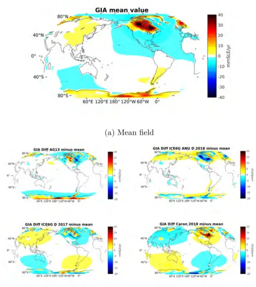
the Glacial Isostatic Adjustment (GIA) correction, both being applied to GRACE data.

This is particularly true for the ocean mass and glacier andTWS mass change estimates for which the uncertainty in trends for the period from 2005 to 2015 is ±0.33 mm SLE/yr. Regarding the glacier and TWS mass change at basin scale, I identify glacier leakage as the main source of uncertainty at local scale in regions close to glaciers. I propose a method using non-GRACE-based mass estimates to reduce the leakage uncertainty on the

GRACE-based local water mass estimate. Accounting for glacier mass changes derived

from satellite imagery leads to improved estimates of other hydrological processes affecting the local water cycle.

Regarding the ocean mass, I explore a method in view of improving the estimates of the ocean mass by working in a reference frame centered at the center of mass of the Earth , the goal being to remove the geocenter correction and the associated uncertainty. I analyse the consistency between GRACE-based ocean mass, altimetry-based sea-level, and ARGO-based steric sea level. This work enables the improvement the estimates of the ocean mass changes. It further leads to a better closure of the sea level budget and a more accurate estimate of theEEI.

Keywords: Global water budget, Ocean mass, Space gravimetry, Climate change, Space Geodesy.

l’eau bas´ees surGRACE est donc mal caract´eris´e. Ce qui entrave l’estimation pr´ecise des changements dans la quantit´e total d’eau dans les continents et dans la masse de l’oc´ean conduisant `a une contribution incertaine de la masse de l’oc´ean `a l’´el´evation du niveau de la mer et `a une estimation incertaine du d´es´equilibre ´energ´etique de la terre, lorsqu’elle est estim´ee par l’approche bilan globale du niveau de la mer.

Au cours de ma th`ese, je revisite le traitement des donn´ees satellitairesGRACE dans le but d’obtenir des estimations du bilan global de l’eau, `a des ´echelles interannuelles `a d´ecennales, en accordant une attention particuli`ere aux diff´erentes sources d’erreurs et d’incertitudes. Je prends en compte tous les post-traitements les plus `a jour des donn´ees

GRACE, `a partir desquels je d´eveloppe un ensemble de solutions GRACE coh´erentes pour estimer les changements de masse au Groenland, en Antarctique, dans l’oc´ean et dans le reste des terres ´emerg´ees y compris les glaciers et les eaux terrestres. Avec cet ensemble, j’analyse la nature des ´echanges de masse d’eau entre l’oc´ean et les continents, et j’´evalue les incertitudes associ´ees. L’amplitude de l’incertitude explique les diff´erences entre les estimations pr´ec´edentes des composantes du bilan global de l’eau effectu´ees `a partir des donn´ees GRACE. Cette approche permet donc d’explorer les sources d’incertitudes dans ces estimations.

J’estime que les diff´erents post-traitements sont responsables de 79% de l’incertitude sur les estimations du bilan global de l’eau, tandis que seulement 21% est dˆu aux diff´erences entre les processus d’inversion des donn´eesGRACE. Les principales sources d’incertitudes dans le bilan global de l’eau bas´e sur GRACE, `a des ´echelles de temps annuelles `a inter-annuelles sont la dispersion dans les corrections du mouvement du g´eocentre ainsi qu’`a l’incertitude dans la correction du rebond post-glaciaire. Cela est particuli`erement vrai pour l’estimation de la masse de l’oc´ean et les eaux continentales dont l’incertitude li´ee `a la tendance pour la p´eriode 2005 `a 2015 est de ±0.33 mm SLE/yr.

En ce qui concerne les variations de masse des glaciers et des eaux continentales, `a l’´echelle d’un bassin, j’identifie les fuites spectrales de masse d’eau depuis les glaciers comme ´etant la principale source d’incertitude dans les r´egions proches des glaciers. Je propose une m´ethode utilisant des estimations de masse non bas´ees sur GRACE afin de r´eduire l’incertitude li´ee `a ce processus. La prise en compte de ces estimations de masse conduit `a une am´elioration des estimations d’autres processus hydrologiques affectant le cycle local de l’eau.

En ce qui concerne la masse globale de l’oc´ean, j’explore une m´ethode pour am´eliorer les estimations, en travaillant dans un r´ef´erentiel avec pour origine le centre de masse de la Terre afin de supprimer l’effet venant de l’incertitude de la correction de g´eocentre. J’analyse la coh´erence entre masse de l’oc´ean bas´ee sur GRACE, le niveau de la mer bas´e sur l’altim´etrie et le niveau st´erique de la mer bas´e sur ARGO. Ces travaux permettent d’am´eliorer les estimations des changements de masse de l’oc´ean et aboutissent ainsi `a une meilleure clˆoture du bilan du niveau de la mer et, finalement, ! `a une estimation plus pr´ecise du d´es´equilibre ´energ´etique de la terre.

Climate is changing. This is nowadays a fact that was still under discussion a few decades ago. Great efforts were deployed at the end of the 20th century in order to characterize key variables of the Earth's system (temperature, sea level rise, total amount of CO2 in the atmosphere, etc.). These efforts revealed that the changes in Earth's climate system were happening at an unprecedented speed during the last decades of the 20th century compared to the previous centuries. In 2007 the International Panel for Climate

Change (IPCC) confirmed that climate change was unequivocal and stated with a very

high confidence the anthropogenic origin of this change. This result was confirmed by

IPCC in 2013 and the anthropogenic origin was stated as extremely likely. However, these facts are still not fully understood by the non-scientific people. There are a lot of shortcuts and half-trues in the media and in our elected leader's speeches. During this PhD, I realized around me that under the concept of climate change, we tend to include the causes and the effects of climate change, as well as several ecological matters as air pollution in the cities, plastic pollution in the seas, lowered biodiversity, etc. Just to clarify this concept, I will try to explain the climate change in plain language.

Earth's climate is driven by the long term response to the energy balance between the input from Sun's radiation and the output from Earth’s radiation. Change in this balance is known as EEI. EEI _{provokes changes in the Earth's climate. Earth's climate}

changes also due to natural reasons such as the changes in the orbit of the earth (known as Milankovic cycles1_{), volcanic activity, tectonics, or biosphere changes. However, since the}

industrial era (1850s), the increase of CO2in the atmosphere has modified this equilibrium. This extra CO2 is preventing radiation to escape the Earth's system. The accumulation of this excess of energy leads to changes in the Earth such as the rise of the global-mean temperature (known as global warming), the rise of sea-level, the melting of glaciers, the changes in the global water cycle, etc. This EEI induced by the increase of CO2 in the atmosphere is known as the human-induced climate change. Measuring these geophysical consequences is key to understand and quantify climate change.

My work has contributed to characterize the exchange of water between ocean and continents since 2002 using satellite data. This exchange is key to understand the sea level rise as well as to understand the evolution of land water under climate change. The knowledge of this exchange with its uncertainties is necessary to improve the understand-ing of climate change consequences and to improve the validation of climate models used to predict climate evolution for the 21st century and beyond.

This manuscript is composed of five chapters.

The first chapter introduces the global water budget and sea-level budget. I present the state of the knowledge and the challenges to improve this knowledge. I do not include any own result in this first chapter. At the end, I summarize the main scientific questions addressed in this PhD.

The second chapter focuses on the global water budget estimates from the GRACE

mission which is arguably the most accurate and comprehensive tool to estimate the global water budget. I analyze the limitations and advantages of the GRACE-based estimates

1

chapter.

In the fourth chapter, I move to the ocean part of the global water budget. On the basis of my ensemble of GRACE solutions, I focus on the geocenter motion correction and the GIA correction as the major sources of uncertainty in the ocean mass changes. I explore a method to improve the estimates of the ocean mass by removing the uncertainty in geocenter. This work has implications not only for the ocean mass estimates but also for the sea level budget and for the EEI.

In the fifth chapter, I discuss the conclusions and explore perspectives for the next years in terms of improvement of our knowledge of the global water cycle using GRACE

and the next gravimetry mission measurements

I also include 2 annexes to this manuscript to assist the reader through this work: • Annex A includes the abstracts of the publications I coauthored without being first author.

• Annex B explains the use of the stokes coefficients for gravity and water mass redis-tribution.

Le climat change. Aujourd’hui c’est un fait; mais il ´etait encore en discussion il y a quelques ann´ees. A la fin du XX`eme si`ecle, d’importants efforts ont ´et´e d´eploy´es dans le but de caract´eriser les variables cl´es du syst`eme Terre : la temp´erature, l’´el´evation du niveau de la mer, la quantit´e totale de CO2 dans l’atmosph`ere, etc. Ces efforts ont r´ev´el´e que les changements dans le syst`eme climatique terrestre se produisaient `a une vitesse sans pr´ec´edent au cours des derni`eres d´ecennies du XX`eme si`ecle par rapport aux si`ecles pr´ec´edents. En 2007, le IPCCa confirm´e que le changement climatique ´etait sans ´equivoque; et il a d´eclar´e avec une tr`es haute confiance l’origine anthropique de ce changement. Ce r´esultat a ´et´e confirm´e ensuite parIPCCen 2013 et l’origine anthropique a ´et´e d´eclar´ee comme extrˆemement probable. Cependant, ces faits ne sont pas encore pleinement compris par les politiques et le grand public. Il y a encore beaucoup de raccourcis et de demi-v´erit´es dans les m´edias ainsi que dans les discours de nos ´elus. Au cours de ma th`ese, j’ai r´emarqu´e que derri`ere le concept de changement climatique, nous avons tendance `a inclure les causes et les effets du changement climatique, ainsi que plusieurs questions ´ecologiques comme la pollution de l’air dans les villes, la pollution plastique dans la mer, la diminution de la biodiversit´e, etc. Pour clarifier le concept, je vais essayer ici d’expliquer le changement climatique en langage clair.

Le climat de la Terre est r´egi par la r´eponse sur le long terme au bilan ´energ´etique entre apport par le rayonnement solaire et perte par le rayonnement terrestre. La modification de cet ´equilibre est connue sous le nom de d´es´equilibre ´energ´etique de la Terre ou EEIen anglais. Le d´es´equilibre ´energ´etique de la terre provoque des changements dans le climat de la Terre. Mais des changements sont egalement dus `a des raisons naturelles telles que les changements dans l’orbite de la Terre (connus sous le nom de cycles de Milankovic

2_{), l’activit´e volcanique, la tectonique ou les changements de la biosph`ere. Cependant}

depuis l’`ere industrielle (environ 1850), l’augmentation de CO 2 dans l’atmosph`ere a modifi´e cet ´equilibre, car le CO 2 suppl´ementaire empˆeche le rayonnement de s’´echapper du syst`eme Terre. L’accumulation de cet exc`es d’´energie entraˆıne des changements dans la Terre tels que l’augmentation de la temp´erature moyenne mondiale (connue sous le nom de r´echauffement climatique), l’´el´evation du niveau de la mer, la fonte des glaciers, des changements dans le cycle global de l’eau, etc. Ce d´es´equilibre ´energ´etique de la Terre induit par l’augmentation du CO 2 dans l’atmosph`ere, est connu sous le nom de changement climatique d’origine antropique. Mesurer ses cons´equences g´eophysiques est devenu essentiel dans le but de comprendre et quantifier le changement climatique.

Mon travail s’inscrit dans ce domaine et se base essentiellement sur des donn´ees satelli-taires acquises depuis 2002; il vise `a comprendre l’´el´evation du niveau de la mer ainsi que l’´evolution des eaux continentales sous l’effet du changement climatique. La connaissance de cet ´echange avec ses incertitudes est n´ecessaire pour am´eliorer la compr´ehension des cons´equences du changement climatique, valider les mod`eles climatiques et diminuer si possible les incertitudes dans le but de faire des pr´evisions sur l’´evolution du climat aussi fiables que possible pour les d´ecennies `a venir.

J’ai choisi de r´ediger Ce manuscrit en anglais mais le r´esum´e, la preface ainsi que les conclusions sont ´egalement en fra¸cais. Le document est compos´e de cinq chapitres dont

2

Dans le troisi`eme chapitre, je m’int´eresse `a l’´echelle r´egionale (continentale). J’utilise l’ensemble de mes solutionsGRACEpour analyser les incertitudes sur les estimations des eaux continentales issus duGRACE `a l’´echelle du bassin. J’identifie la fuite des glaciers dans les solutionsGRACEcomme la principale source d’incertitude `a l’´echelle locale dans les r´egions proches des glaciers. Je propose une m´ethode utilisant des estimations de masse non issues de GRACE afin de r´eduire l’incertitude de fuite sur les estimations locales de masse d’eau bas´ees sur GRACE. Je teste et je valide cette m´ethode en Asie du Sud, une r´egion o`u les glaciers et les lacs sont concentr´es dans de des localisations de faible ´etendue. La prise en compte de leurs changements de masse permet d’am´eliorer les estimations d’autres processus hydrologiques affectant le cycle de l’eau local. Ce chapitre est bas´e sur un article en pr´eparation Blazquez et al. [In prep2020], qui est joint `a la fin du chapitre.

Dans le quatri`eme chapitre, je m’int´eresse `a la partie oc´eanique du bilan global de l’eau. Sur la base de mon ensemble de solutionsGRACE, j’identifie la correction de mouvement du g´eocentre et la correction GIA comme ´etant les principales sources d’incertitude dans les changements de masse oc´eanique. J’explore une m´ethode pour am´eliorer les estima-tions de la masse oc´eanique en m’affranchissant de l’incertitude sur le g´eocentre. Ce travail a des implications non seulement pour les estimations de la masse oc´eanique, mais aussi pour le budget du niveau de la mer et pour le d´es´equilibre ´energ´etique de la Terre. Dans le cinqui`eme chapitre, je discute les conclusions et explore les perspectives pour les prochaines ann´ees en terme d’am´elioration de notre connaissance du cycle global de l’eau, en utilisant GRACE et les measures de la prochaine mission de gravim´etrie.

J’inclus ´egalement 2 annexes `a ce manuscrit pour aider le lecteur `a travers ce travail: • L’annexe A comprend les r´esum´es des publications que j’ai co-´ecrites sans ˆetre le premier auteur.

• L’annexe B explique l’utilisation des coefficients de Stokes pour la redistribution de la gravit´e et des masses d’eau.

Abstract i

[Fr] R´esum´e ii

Foreword iii

[FR] Pr´eface v

1 Introduction: Water cycle and sea level 1

1.1 Water cycle . . . 1

1.2 Land water mass change . . . 3

1.2.1 Greenland and Antarctica . . . 3

1.2.2 Glaciers . . . 6

1.2.3 Terrestrial water storage . . . 8

1.3 Ocean mass change . . . 10

1.3.1 Ocean mass from the global water budget . . . 10

1.3.2 Ocean mass from gravimetry . . . 10

1.3.3 Ocean mass from the sea level budget . . . 11

1.3.3.1 Sea-level change . . . 12

1.3.3.2 Steric sea-level change . . . 14

1.3.3.3 Ocean mass derived from the sea-level budget . . . 15

1.3.4 Ocean mass from the fresh-water budget . . . 15

1.4 Global energy budget and how it relates to the water cycle . . . 16

1.5 Scientific questions associated to the water cycle . . . 17

1.6 Objectives of this PhD . . . 18

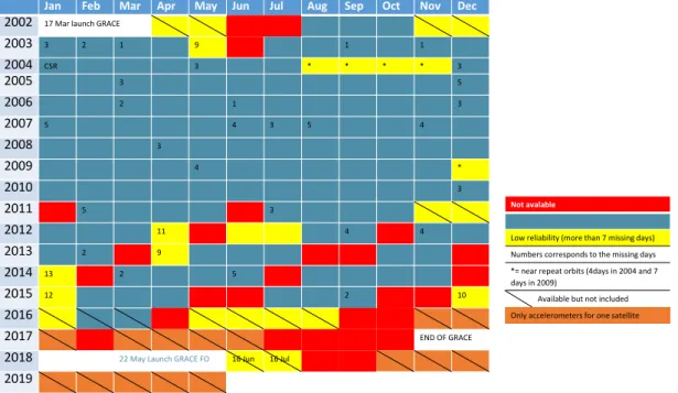
2 Evaluating the uncertainty in GRACE-based estimates of the global water budget. Development of an ensemble approach 21 2.1 GRACE and GRACE FO missions . . . 22

2.1.1 Inversion process (From L1 data to L2 products) . . . 23

2.1.2 Post-processing (From L2 products to water mass anomalies) . . . . 25

2.2 GRACE Post-processing . . . 26

2.2.1 Geocenter motion . . . 26

2.2.2 Earth’s dynamic oblateness . . . 28

2.2.3 Stripes . . . 29

2.2.4 Leakage and Gibbs effect . . . 31

2.2.5 Glacial isostatic Adjustment . . . 33

2.2.6 Pole tide . . . 35

2.2.7 Earthquakes . . . 37

2.3 Applications of the ensemble of GRACE solutions . . . 39

2.3.1 Comparison of the global water budget components with previous studies . . . 39

2.3.2 The global water budget and its uncertainties analyzed with my ensemble of GRACE solutions . . . 39

3.2.1 Glaciers at global scale . . . 93

3.2.2 Land Water Storage (LWS) at global scale . . . 94

3.3 Conclusion . . . 97

4 Uncertainty in GRACE-based estimates of the ocean mass. Implications for the sea level budget and the estimation of the EEI 99 4.1 Impact of the choice of the reference frame on the ocean mass estimate from GRACE . . . 100

4.2 Implications on the Sea level budget . . . 102

4.2.1 Altimetry sea-level change . . . 102

4.2.2 ARGO-based steric sea-level . . . 103

4.2.3 Consistency in the sea-level budget . . . 105

4.3 Implications for the EEI . . . 108

4.4 Conclusions . . . 109

5 Conclusions and outlook 111 6 [FR] Conclusions and perspectives 117 Bibliography 120 Acronyms 135 List of figures 138 List of tables 141 Annex A: Abstracts of the articles not included in the main text i A1: Arctic Sea Level During the Satellite Altimetry Era . . . i

A2: Mass Balance of the Antarctic Ice Sheet from 1992 to 2017 . . . ii

A3: Global Sea-Level Budget 1993–Present . . . iii

A4: Measuring Global Ocean Heat Content to Estimate the Earth Energy Imbalance . . . iv

A5: Global Ocean Freshening, Ocean Mass Increase and Global Mean Sea Level Rise over 2005–2015 . . . v

A6: Mass Balance of the Greenland Ice Sheet from 1992 to 2017 . . . vi

Annex B: Stokes coefficients vii B1: Stokes coefficients description . . . vii

Introduction: Water cycle and sea

level

1.1

Water cycle

The water cycle refers to the water transformation, transportation and storage in the Earth’s system. It is mainly driven by the solar heating which evaporates the water from the ocean and land surfaces and melts the ice from land and from the ocean. The evaporated water condensates and precipitates over land and the ocean. The precipitated water over land may be accumulated or transported back to the ocean closing the cycle. This water cycle is well characterized at global and annual scale (Fig. 1.1) [ Tren-berth, 2014]. However, changes at interannual and longer time scales are less well known [Stephens and L’Ecuyer, 2015;Wild et al.,2015;Rodell et al.,2015]. In this PhD, I focus on the interannual to decadal changes in the water cycle.

Earth is a massive planet whose gravity is large enough to prevent the water vapor from escaping through the top of the atmosphere. However it is not big enough to prevent a small loss of hydrogen of about 3 kg/s [Catling and Zahnle,2009]. This loss of hydrogen represents the main variation of the Earth’s mass at annual and longer time scales. The rate of hydrogen loss represents a mass loss of 10-7 _{Gt/yr. As water molecules are made} up of hydrogen and oxygen (H2O), this hydrogen mass loss provoke a water mass loss of 9 · 10−7 Gt/yr and an increase of oxygen mass in the atmosphere of 8 · 10−7 Gt/yr1_{. In}

this PhD, I focus on the storage terms of the water cycle and the maximum accuracy I will need in terms of mass is 10-1_{Gt/yr. So, I assume here the total amount of mass and} water in the Earth’s system remains constant at interannual to decadal time scales.

Water vapor remains mainly in the lower part of the atmosphere, in the Troposphere essentially. The amount of water vapor in the atmosphere varies very quickly at daily and seasonal time scales and also depending on orography and temperature. At a global scale, the water-holding capacity mainly changes depending on the average temperature (See Clausius-Clapeyron law at Eq. 1.1,where es is the water-holding capacity). When

Figure 1.1: Observations (black numbers) and reanalysis (color numbers in the boxes) estimates of the water cycle fluxes in 103Gt/yr and storages in 103Gt. Excerpt from [Trenberth, 2014].

linearized, the water-holding capacity increases by about 6-7% per extra degree Celsius in global surface temperature (Eq. 1.1).

In the last 60 years surface temperature has increased by 0.72 ◦Celsius in response to climate change [e.g., Hartmann et al., 2013]. Assuming a total water vapor content in the atmosphere of 12.7 103_{Gt [Trenberth, 2014], the amount of water in the atmosphere} is expected to increase in response to climate change at a rate of 10 Gt/yr. This rate is of greater than the maximum accuracy I will need in term of mass (10-1 _{Gt/y) to analyze} the changes in the water storage terms of the water cycle. However, as I will show in the next chapters, this accuracy is beyond the actual limits. So I assume atmospheric water mass to remain constant at interannual to decadal time scales.

es(T ) = 6.112 · e 17.64T T +243.5 ∆Matm Matm ' 6 − 7% ∆Tadimensional (1.1)

Under these assumptions, the global water budget may be expressed as the water mass exchange between land and the ocean (Eq.1.2). We analyze the land components of the water cycle in Section 1.2 and the ocean component in Section 1.3.

1.2

Land water mass change

Land water mass is composed of ice, snow, soil moisture, water in the biosphere, groundwater and surface water (including rivers, glaciers and lakes). However, as the In-ternational Panel for Climate Change (IPCC), we prefer to break down the land storage geographically (Greenland and Antarctica) and by the water state (glaciers and terres-trial water storage), although terresterres-trial water storage includes solid water from snow, permafrost and ice on lakes and rivers and the ocean includes solid water from sea ice. The global water budget may be expressed as the sum of the ocean, Greenland, Antarc-tica, glaciers, and Terrestrial Water Storage (TWS) mass changes (Eq. 1.3). Hereafter, I will adopt the following convention: a negative value of the mass change means a land mass loss expressed in Gt and its equivalent ocean mass increase expressed in mm

Sea-Level Equivalent (SLE). Note that cubic kilometers, gigatons and mm SLE are common

units used to describe an amount of water mass, usually assuming the density of the water as the density of freshwater

1km3 ∼ 1Gt = 1012_{kg ∼} 1

360mmSLE .

∆Mocean(t) + ∆MGreenland(t) + ∆MAntarctica(t) + ∆Mglaciers(t) + ∆MT W S(t) = 0 (1.3)

1.2.1

Greenland and Antarctica

The Greenland and Antarctica ice sheets and peripheral glaciers play a major role in the water cycle at interannual and longer time scales. They are by far the largest reservoirs of freshwater. Antarctica contains 25.71 · 106 _{Gt (∼58.3 m SLE) and Greenland 2.85 · 10}6 Gt (∼7.36 mSLE) [Vaughan et al.,2013]. Nearly at equilibrium until the 90s (Fig. 1.2), they became major contributors to the sea level rise in the last decades [Bamber et al.,

2018;Cazenave et al., 2018a].

The mass loss from both ice sheets is estimated by satellite altimetry (since 1991), satellite gravimetry (since 2002), and theIOM (since 1979).

Satellite altimetry includes radar altimetry (since 1993), laser altimetry (only 7 years) andSynthetic Aperture Radar (SAR)(since 2010). Satellite altimetry provides ice sheets elevation anomalies which are converted to mass changes using ice density and firn-layer thickness. The precision of the elevation anomalies relies on modest adjustments to ac-count for sensor drift, changes in the satellite attitude, atmospheric attenuation, and movements of Earth’s surface. The conversion from elevation anomalies to mass change remains the main source of uncertainty as it depends on external models of fluctuations in the firn-layer thickness [Shepherd et al., 2012]. This conversion is performed by us-ing a prescribed density model and by allowus-ing for temporal fluctuation in the snowfall. Mass change observation using radar altimetry are continuous since 1991 with: ERS 1 (Jul 1991-Mar 2000), ERS2 (Apr 1995-Jun 2003), Envisat (Mar 2002-Apr 2012) and Sen-tinel 1 (Apr 2014-present). Laser altimetry fromIce, Cloud, and land Elevation SATellite

(WAIS), and Antarctic Peninsula (AP) [Schr¨oder et al., 2019]. Altimetry-based EAIS

mass balance trend for the period from 1992 to 2017 is between [-11 to 136] Gt/yr,WAIS

mass balance trend is about [-97 to -25] Gt/yr for the same period and AP mass balance trend is about [-29 to 3] Gt/yr for the same period [Shepherd et al., 2018].

Mass changes using gravimetry are available since 2002 with Gravity Recovery and

Climate Experiment (GRACE) (Apr 2002-Jun 2016) and Gravity Recovery and Climate

Experiment Follow On (GRACE FO) (Jun 2018 - present). Once corrected for

non-water mass anomalies, the gravity field may be converted to non-water mass anomalies. It complements the local data from altimetry in a monthly time scale and a 300 km spatial resolution. Main sources of uncertainty in the mass estimates based on this technique are:

Glacial Isostatic Adjustment (GIA)correction, especially for Antarctica, and land/ocean leakage correction (especially at AP and Greenland) (see chapter 2).

For the period from 2005 to 2015, GRACE-based Greenland mass change trends of −249 ± 23 Gt/yr agrees with altimetry estimates of −235 ± 37 Gt/yr [Shepherd et al.,

(a) Greenland. Excerpt from Bamber et al. [2018]

(b) Antarctica mass balance estimated by the Input-Output Method (IOM) (purple) and its components: surface mass balance (blue) and ice discharge (red). Excerpt from Rignot et al.[2019]

Figure 1.2: Cumulative mass balance for Greenland (a) and Antarctica (b) from different techniques

2019]. Mass balance trends are between [11,107] Gt/yr for EAIS, [-174,-114] Gt/yr for

WAIS, and [-39 to -9] forAP [Shepherd et al., 2018]. Rapid melting in Greenland during summer 2012 and the extreme snow accumulation on winter 2013 explains most of the differences in trends when considering different time spans [Bamber et al., 2018]. Over the period from 2002 to 2015 Greenland mass loss was 265 ± 25 Gt/yr [Wouters et al.,

2019].

The Input-Output Method (IOM)consists in quantifying ice discharge into the ocean, and theSurface Mass Balance (SMB).SMBis the difference between mass gained through snowfall and lost by sublimation at the surface and by melt-water runoff. This method has the advantage of explaining the mass changes in ice sheet and glaciers at drainage basin scale and on monthly basis but its accuracy relies on the models used. The spread in IOM trend estimates are ±71 Gt/yr for Greenland mass change and ±82 Gt/yr for Antarctica mass change, considerably larger than the spread in altimetry and gravimetry mass changes (See Table 1.1). Recently extended, IOM provides mass loss estimates for Greenland since 1972 [Mouginot et al., 2019] and for Antarctica since 1979 [Rignot et al.,

2019]. These publications use an update drainage inventory, ice thickness, and ice velocity data to calculate the basin grounding line ice discharge.

IOM-based Greenland mass balance is estimated at −102 ± 20 Gt/yr for the period 1972 to 2018 with clear decadal variations. Greenland mass balance was positive in the 70s with a trend of 47 ± 21 Gt/yr, then it became negative in the 80s with a trend of −51 ± 17 Gt/yr due to an increase of solid ice discharge [Mouginot et al., 2019]. It remained negative in the 90s with a trend of −41 ± 17 Gt/yr. In the decades 2000-2009 and 2010-2019, the Greenland mass loss increased to trends of −187 ± 17 Gt/yr and −286 ± 20 Gt/yr, respectively. It was due to abrupt changes due to a decrease in the

SMB and an increase of solid ice discharge [e.g., Mouginot et al., 2019]. SMB explains most of the interannual variability, especially the strong negative mass balance in 2012 which was due to an increase in melt-water runoff [van den Broeke et al., 2016]. On the other hand, solid ice discharge and the mass loss of peripheral glaciers mostly contribute to the trend. Most of the mass loss take place in the low elevations (below 2000 m a.s.l.) near the coast (the first 150 km) [van den Broeke et al., 2016].

The total mass balance from Antarctica decreased from −40 ± 9 Gt/yr in the 11-yr time period 1979–1990 and −50 ± 14 Gt/11-yr in 1989–2000 to −166 ± 18 Gt/11-yr in 1999–2009, and −252 ± 26 Gt/yr in 2009–2017 [Rignot et al., 2019]. SMB in Antarcatica has been nearly at equilibrium because temperature remains negative except some glaciers in Antarctic peninsula. West Antarctica and Antarctic peninsula mass loss is dominated by the increase in solid ice discharge while solid ice discharge is a minor contribution to the East Antarctica mass balance (Fig.1.2b andShepherd et al.[2018]). Compared to the other techniques, Greenland and Antarctica mass loss, estimated by IOM present higher mass loss rate and not always in agreement (Table 1.1).

Greenland and Antarctica have become dominant contributors of the global water budget since the beginning of 21st century [Church et al., 2013]. All projections for 21st century foresee that they will remain the main contributor with an expected contribution at the end of 21st century from 0.11 [0.01 to 0.24] m SLE for RCP2.6 to 0.16 [0.01 to 0.33] for RCP8.5 [Church et al., 2013], or even higher values proposed by a structured expert judgment leading to 0.22 [0.05 to 0.51] m SLE for RCP2.6 to 0.49 [0.23 to 1.02]

weather conditions (0.06 m in RCP2.6 to 0.13 m in RCP8.5) and the Antarctic ice sheet dynamics response (0.17 m in all scenarios). Recently analyzed, marine ice cliff instability may increase Antarctic contribution between 0.26 to 0.58 m and 0.64 to 1.14 m GMSL by 2100, for RCP4.5 and RCP8.5, respectively [DeConto and Pollard, 2016; Kopp et al.,

2017; Edwards et al., 2017].

1.2.2

Glaciers

There are around 215 000 glaciers in the last inventory: RGI 6.0 [RGI Consortium,

2017]. They correspond to a water reservoir of 0.158 ± 41 · 106 Gt (∼ 0.32 ± 0.08 m

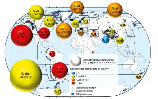
SLE) [Farinotti et al., 2019]. From the middle of the 19th centery (around the end of the little ice age) glacier contribution has dominated the global water budget until the 21st century when Greenland contribution became larger [Leclercq et al.,2014; Marzeion et al., 2017]. Glacier mass changes in response to surface temperature and precipitations changes. Most of the glaciers are losing mass, although a few are nearly at equilibrium or even gaining mass (See South Asia in Fig. 1.3).

Glacier mass loss may be estimated with the same techniques as Greenland and Antarc-tica ice sheets (altimetry, gravimetry and IOM), but the size of the glacier, their topog-raphy, and the large number of glaciers hampers the generalization of these techniques [Marzeion et al., 2017]. Instead, there are specific techniques to estimate glacier mass change based on the glacier length, in situ direct observations (glaciological), and volume change with airborne and high resolution satellite imagery (geodetical) [Cogley et al.,

2010].

Gravimetry is used globally and at monthly scale to retrieve glacier mass anomalies as for ice sheets mass changes. Once corrected for the non-water mass anomalies, gravity field is converted to water mass anomalies. However, retrieving glacier mass changes needs to separate hydrological and glacier signals and to reduce the uncertainty due to the spatial resolution. The first attempts to estimate the glacier mass changes by gravimetry assumed the hydrology beneath and around the glacier negligible [Chen et al.,2013;Yi et al.,2015]. Next studies included hydrological models to correct for the hydrological mass changes [Jacob et al.,2012;Gardner et al.,2013;Schrama et al.,2014] and recent studies combine hydrological models for some regions and considered hydrology negligible for other regions [Reager et al.,2016;Rietbroek et al.,2016;Bamber et al.,2018;Wouters et al.,2019]. The other drawback of using gravimetry to retrieve glaciers is the spatial resolution (about

Figure 1.3: Regional glacier contributions to sea-level rise from 1961 to 2016. The cumulative regional and global mass changes (in Gt, represented by the volume of the bubbles) are shown for the 19 regions (outlined with bold black lines from Randolph’s Glacier Inventory (RGI) 6.0). Specific mass-change rates (m water equivalent yr−1) are indicated by the colors of the bubbles. Excerpt fromZemp et al. [2019].

300 km) much larger than glaciers (a few km). There are currently two methods to reduce the uncertainty in the glacier mass estimates: forward modeling [Chen et al., 2013; Yi et al., 2015] and mascons [Jacob et al., 2012; Gardner et al., 2013; Schrama et al., 2014;

Rietbroek et al., 2016; Reager et al., 2016; Wouters et al., 2019] although both methods seems to overestimate small glaciers as in Alps or in High Mountain Asia (HMA) [Long et al.,2016]. We discuss the use of gravimetry to estimate glacier mass changes in detail in chapter 3. Globally, gravimetry-based glacier estimate a trend of −183 ± 54 Gt/yr for the period 2003-2009 in glacier mass change, which is smaller than the trends retrieved from other techniques (between -216 and -342 Gt/yr from Table 1.2).

Table 1.2: Global glacier mass trends estimated from different techniques. Values are expressed in Gt/yr. Excerpt from Marzeion et al. [2017] with the addition of estimates fromZemp et al. [2019]

Technique Reference 2003-2009 1961-2010

Gravimetry-based glacier [Marzeion et al.,2017] −183 ± 54a

Spatially-weighted in situ mass change observations [Zemp et al.,2019] −342b ₋₂₀₅ Spatially-weighted in situ mass change observations [Cogley,2009] −234 ± 25b _{−194 ± 18}

Glacier length change [Leclercq et al.,2014] −266 ± 230b _{−209 ± 54}

Mass budget from different methods [Gardner et al.,2013] −216 ± 25b

Glacier modeling [Marzeion et al.,2017] −244 ± 54b _{−176 ± 18} a_{Averaged over different time periods (2002/2005–2013/2015)}

b _{Greenland peripheral glaciers removed fromGardner et al.[2013]}

Glacier mass change is also estimated through the glacier length observations for some glaciers (i.e. 471 inLeclercq et al.[2014]). A few of these in situ observations are available since mid 1850s. However, to convert the length changes into mass changes, it is necessary

There is a good agreement in estimates of global glacier mass trend for the period from 2003 to 2009 among most of the techniques around −244±33 Gt/yr, except from gravime-try and direct mass change observations. Gravimegravime-try-based estimates are less negative −183 ± 54 Gt/yr while estimates derived from direct observations are more negative −342 Gt/yr (Table 1.2). For the period from 1961 to 2010, glacier mass trend estimated by direct mass observation of −205 Gt/yr shows a better agreement with estimates from the glacier length change.

Glaciers are not included in climate models because the processes that drive their mass changes are too small scale to be resolved by climate models. Instead, climate models outputs are used to force offline glacier models allowing to project future glacier contribution to sea level rise [e.g., Marzeion et al., 2015]. Depending on the scenario, glacier contribution to sea-level rise at the end of the 21st century is 0.10 [0.04 to 0.16] m SLE for RCP2.6 to 0.16 [0.09 to 0.23] for RCP8.5 [Hock et al., 2019]. The uncertainties of ±0.12 m SLE is smaller than the Greenland and Antarctica contribution uncertainty, and mainly due to the downscaling from climate models [Church et al., 2013]. Glacier contribution is expected to decrease as glaciers retreat to higher mountains and some glaciers are disappearing during the 21st century.

1.2.3

Terrestrial water storage

The Terrestrial Water Storage (TWS) includes the water from the emerged land not

included in glaciers nor in ice sheets i.e.: ice, snow, soil moisture, water from the biosphere, groundwater and surface water (including rivers, lakes and dams). Groundwater mass down to 4000m is estimated at 15.300 · 106 _{Gt (∼ 42.5 m SLE) and the rest of TWS} is estimated at 0.32 · 106 _{Gt (∼ 0.88 m SLE)[Trenberth, 2014]. TWS is responsible for} most of the ocean mass variability at annual and interannual scale e.g.[Wada et al.,2016]. Changes in TWShappens in response to natural variability (e.g. El Ni˜no, North Atlantic Oscillation (NAO), volcanoes, etc.) and to direct human-induced effects (dams, irrigation, water pumping, etc.) [Scanlon et al., 2018]. Climate change induced effects on TWS

changes have not been yet detected in the last decades because of the large uncertainties in TWS changes and the large natural variability [Fasullo et al., 2016a; Kusche et al.,

2016].

Due to the large surface of continents, it is very difficult to get a global measurement of the mass changes inTWS. Some authors focus in one component like: snow [Biancamaria

et al.,2011], groundwater measured by wells [Asoka et al.,2017], surface water from dams [Wada et al.,2016] or lakes [Cretaux et al.,2016]. Other authors focus on specific regions like Mississippi basin [Rodell et al., 2004]. Seasonal and interannual TWS mass changes dominate the TWS mass changes at basin scale while trends are at least one order of magnitude smaller [Scanlon et al., 2019]. Spatially, there are also great differences from one basin to another depending on the topography, on local precipitations, on human activities, on policies, etc. [Scanlon et al., 2018]. The differences in order of magnitude and spatial variability hamper trend and interannual variability extrapolation from one basin to another.

The only observing system that provides globalTWSmass change estimates isGRACE

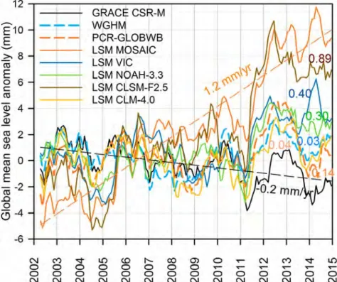
but there are great discrepancies among theTWSestimates. Based on the 200 main basins (around 60% of theTWS surface), some authors suggests a water mass accumulation in continents for the period 2002-2014 between 118 Gt/yr [Reager et al.,2016] and 77 [71 to 82] Gt/yr [Scanlon et al., 2018]. While others authors suggests a mass loss of −79 ± 93 Gt/yr for the same period [Rietbroek et al.,2016].

Mass trends for the same period based on hydrological models are negative −118 ± 64 Gt/yr [Dieng et al., 2017] or [-450 to -12] Gt/yr [Scanlon et al., 2018]. Differences are partially explained by some mismodeling in the hydrological models, especially the lack of surface water and groundwater terms or the lack of direct human-induced effects in

Figure 1.4: GRACE-based TWS contribution to the sea-level (black lines), global hy-drological and water resources models (PCR-GLOBWB and WGHM) and land surface models (MOSAIC, VIC, NOAH-3.3, CLSM-F2.5, and CLM-4.0). Numbers in the figure corresponds to trends for the period from 2002 to 2015. Note that in the figure positive numbers means positive contribution to sea-level and negative mass balance for theTWS. Excerpt from [Scanlon et al., 2018]

1.3

Ocean mass change

The ocean represents the largest reservoir of water containing 97.5% of the total amount of water mass and covering 70% of the Earth’s surface. Observing the ocean is key to understand the changes in the global water cycle because it integrates changes in land ice and land water. The ocean mass is the sum of land mass contributions and as such it can be estimated by adding together the independent estimates of each land mass change (Eq.

1.3). It can also be estimated directly through gravimetry from GRACE, and indirectly via the sea level budget and the ocean freshwater budget. We discuss each method and their estimates in the next subsections.

1.3.1

Ocean mass from the global water budget

Ocean mass estimated via the global water budget is computed as the sum of land mass contributions (Eq.1.3). In this way, the uncertainty in this estimate relies on the uncertainty of each land contribution. The uncertainty is important because of the lack of TWS mass change observations (Section 1.2.3). The 20th century ocean mass trend is estimated via the global water budget at 0.58 [0.41 to 0.73] mm SLE/yr for the period from 1900 to 1991 [Church et al.,2013]. Based on this approach, the ocean mass trend for the period from 1958 to 2014 has been reconstructed to 0.74±0.10 mm SLE/yr [Frederikse et al., 2017].

Ocean mass projections for the 21st century are also estimated via the global water budget between 0.25 [0.04 to 0.49] m SLE in RCP2.6 to 0.36 [0.09 to 0.65] m SLE in RCP8.5 [Church et al.,2013]. Under the assumption that the uncertainties of the different land contributions are not correlated, the uncertainty is estimated as the squared sum of the uncertainties of each contribution (detailed in Section1.2). Following this calculation, the uncertainty in the projections is mainly due to the uncertainty in the Greenland and Antarctica contributions, and more specifically in the Antarctic rapid ice sheet dynamics’ contribution (uncertainty of ±0.17 m SLE).

1.3.2

Ocean mass from gravimetry

There are two main methods to retrieve ocean mass from gravimetry: (1) Quantifying ocean mass change using an ocean basin mask (also called kernel) which excludes coastal

Table 1.3: Published trends of the global water budget (Eq 1.3) in mm SLE/yr. Ocean mass and land contributions from Greenland , Antarctica, glaciers and TWS. Note that the periods are slightly different for each publication and all uncertainties are expressed at 90 %CL.

Source Period Ocean mass Greenland Antarctica Glacier TWS

[Reager et al.,2016] Apr 2002-Dec 2014 1.58 ± 0.43a _{0.77 ± 0.13 0.49 ± 0.53 0.65 ± 0.09 −0.33 ± 0.12} [Rietbroek et al.,2016] Apr 2002-Jun 2014 1.08 ± 0.30a _{0.73 ± 0.03 0.26 ± 0.07 0.38 ± 0.07 0.22 ± 0.26} [Yi et al.,2015] Jan 2005-Jul 2014 2.03 ± 0.22a _{0.77 ± 0.05 0.60 ± 0.18 0.58 ± 0.03 0.07 ± 0.11} [Dieng et al.,2017] Jan 2004-Dec 2015 2.24 ± 0.16b _{0.82 ± 0.10 0.33 ± 0.10 0.58 ± 0.10 0.33 ± 0.18} [Chambers et al.,2017] Jan 2005-Dec 2015 2.11 ± 0.36a

[Chen et al.,2018] Jan 2005-Dec 2016 2.70 ± 0.16a [Chen et al.,2018] Jan 2005-Dec 2016 2.75 ± 0.18b

[Cazenave et al.,2018a] Jan 2005-Dec 2016 2.40 ± 0.40b _{0.76 ± 0.16 0.42 ± 0.16 0.74 ± 0.16 −0.27 ± 0.24} [Blazquez et al.,2018] Jan 2005-Dec 2015 1.63 ± 0.27a _{0.80 ± 0.04 0.63 ± 0.15 0.20 ± 0.31}c [Uebbing et al.,2019] Aug 2002-Jul 2016 1.75 a

[Llovel et al.,2019] Jan 2005-Dec 2015 1.55 ± 1.20d a_{Ocean mass from gravimetry.}

b_{Ocean mass from the sea-level budget.} c_{Glacier andTWS.}

d_{Ocean mass from the freshwater budget.}

areas [e.g., Chambers, 2006a; Chambers and Bonin, 2012] or (2) direct averaging over the whole ocean of a post processed solution that is corrected for leakage [e.g., Rietbroek et al.,2016;Yi et al.,2015;Chen et al.,2018;Reager et al.,2016]. In the kernel approach, coastal ocean areas within certain distance (e.g., 300 or 500 km) from the coast are excluded, in order to minimize leakage signal from land into the ocean and the spatial resolution is degraded to 500 km to reduce the noise. On the contrary, in the direct average over a post-processed GRACE solution, mass changes on land and over ocean are solved at the same time via forward modeling method [e.g., Chen et al., 2018; Yi et al.,

2015], joint inversion with altimetry [e.g., Rietbroek et al., 2016] or mass concentration (mascon) method [e.g., Reager et al., 2016]. Both approaches relies on the correction of non-water mass anomalies that affect the gravity field as earthquakes andGlacial Isostatic Adjustment (GIA). BeingGIA the solid-Earth response to the melting of the continental ice sheets since the last glacial maximum (further details in Section 2.2.5). Ocean mass trends estimates for the last decade ranges from 1.08 ± 0.30 mm SLE/yr [Rietbroek et al.,

2016] to 2.11 ± 0.36 mm SLE/yr [Chambers et al.,2017] and even 2.70 ± 0.16 mm SLE/yr [Chen et al., 2018] (Table 1.3). This large uncertainty of ±1 mm/yr is one of today’s largest uncertainty in the global water budget. The characterization of the uncertainties in the ocean mass is one of the main motivations of my PhD. I will analyze the sources of this uncertainty in the trend estimates by rigorously analyzing all the GRACE post processing (See Chapter2 for more details).

1.3.3

Ocean mass from the sea level budget

The water mass loss from continents run off to the ocean, increasing the ocean mass. As the mass reaches the ocean, it propagates in the ocean leading to an uniform barystatic sea-level rise after 2 to 3 weeks [Lorbacher et al., 2010]. Barystatic sea-level rise (hb) is

1.3.3.1 Sea-level change

GMSLR cannot be directly measured; Instead, GMSLR is computed as the sum of

Global-mean geocentric sea-level rise (GMGSLR) measured with respect to the

Inter-national Terrestrial Reference Frame (ITRF) and the sea floor changes estimated with

respect to the ITRF. These sea floor changes include the sea-floor viscous adjustment caused by past changes in land ice known as GIA correction (hGIA) and contemporary

Figure 1.5: global-mean sea-level rise (Total SSH,Altimetry in the figure), barystatic sea-level rise (Ocean mass in the figure), global-mean thermosteric rise (Thermosteric, ARGO in the figure) and GMSLR (the sum of GRACE + Argo in the figure). Figure excerpt from IPCC AR5 Fig 13-6 [Church et al., 2013]

Earth Gravity, Earth Rotation and viscoelastic solid-Earth Deformation (GRD) (hp)

which accounts for sea-floor elastic adjustment to the ongoing changes in the water trans-port.

GM SLR=GM GSLR− hGIA− hp (Eq.58 f rom Gregory et al.[2019]) (1.6)

GMGSLR is accurately measured (cm resolution every 10 days every 100 km) with

satellite altimeters constellation [Legeais et al., 2018]. Altimeters measure the range between the satellite and the sea surface via the time between the emission and the reception of the radar echo. This range and the satellite position allow to estimate the sea surface height with respect to a geocentric reference ellipsoid. In order to retrieve the sea surface height this measure is corrected for a number of delays in the round travel of the radar echo. The most important delays include the wet Troposphere delay and the ionospheric effect (Further details inEscudier et al. [2017]).

The family of satellite altimeters provides a sea level record of more than 25-year including the records from TOPEX/Poseidon (Aug 1992-Jan 2006), Jason-1 (Dec 2001 – Jun 2013), Jason-2 (Jul 2008 -present), Jason-3 (Jan 2016 -present), as well as those from ERS 1 (Jul 1991-Mar 2000), ERS2 (Apr 1995-Jun 2003), Envisat (Mar 2002 –Apr 2010), SARAL/Altika (Feb 2013- present), Cryosat-2 (Apr 2010-present), HY-2A (Aug 2011-present), Sentinel-3a (Feb 2016-present) and Sentinel-3b (Apr 2018 - present).

TheGIA correction (hGIA) is mainly due to the changes in geoid. GIA affects in many

other ways: (1) the three-dimensional displacements of the Earth’s surface both in the near and in the far field of the former ice sheets, (2) the loading- and un-loading-induced stress variations in the crust and the mantle, and (3) the fluctuations of the Earth’s rotation axis, involving lateral movements of the pole or true polar wander and changes in the length of day (Further details inSpada[2017];Tamisiea [2011]). All these effects must be accounted to estimate theGIA correction applied to altimetry (hGIA) which contributes

about -0.3 mm/yr [Tamisiea, 2011] to the GMSLR. To compute this value, global GIA

models need to account for the change in the barystatic sea-level change sinceLast glacial

maximum (LGM) and its effect on the geoid. There are few GIA models which deliver

this term, leading to a global GIA correction of −0.37 ± 0.05 mm/yr [Stuhne and Peltier,

2015;Peltier et al.,2017]. We will discuss in details this issue in Section 2.2.5.

Contemporary GRD accounts for sea-floor adjustment due to the ongoing changes in the continental water mass. The continental water mass changes cause instantaneous vertical land movement and changes in the geoid due to the elastic deformation of the solid-Earth. As contemporaryGRD and barystatic sea-level are both proportional to the ocean mass (∆MOcean), the sum of both effects has been known in the literature as ocean

fingerprints. Global mean contemporaryGRDreduces global mean sea level rise by about 8% of the barystatic sea-level rise [Frederikse et al., 2017].

GMGSLR has increased with at a rate of 2.8 ± 0.3 mm/yr for the period from 1993 to 2017. Once corrected for GIA (-0.3 mm/yr from Peltier [2004]) and contemporary GRD

(-0.1 mm/yr fromFrederikse et al. [2017]),GMSLRtrend is 3.2 ± 0.3 mm/yr for the same period (Fig1.5). This result is corroborated by an estimation done with tide-gauges along the coast which indicates a trend in GMSLR of 3.2 ± 0.40 mm/yr [Ablain et al., 2015;

analysis of altimetry-based and tide-gauges-based GMGSLR. Uncertainties in the tide-gauges 10-yr trend estimates are ±0.40 mm SLE/yr the period from 1995 to 2005, mainly due to the uncertainties in the vertical land motion near the tide gauges [Ablain et al.,

2018]. The bias calibration induce a temporal correlation in the uncertainty of the trend. Uncertainty in the trend varies from ±0.40 mm SLE/yr for the period from 2002 to 2017 to ±0.35 mm SLE/yr for the period from 1998 to 2018 [Ablain et al., 2019, Figure 5]. Altimetry and tidegauges estimates agrees within 0.07 mm SLE/yr [Ablain et al.,2018]. The agreement between both methods gives high confidence in the uncertainty ofGMSLR

trend.

Projections of sea-level rise for the 21st century are the sum of the projected ther-mosteric sea-level rise and the projected ocean mass (computed through the land mass contributions). They are very dependent on the scenario, varying from 0.44 [0.28 to 0.61] m SLE in RCP2.6 to 0.74 [0.52 to 0.98] m SLE in RCP8.5) [Church et al., 2013]. The uncertainty in the estimates of about [0.33 to 0.46] m SLE comes mainly from the uncer-tainty in the ocean mass [0.25 to 0.34] m SLE and in particular from the unceruncer-tainty in the ice sheet contributions, and to a lesser extent the uncertainty in the thermosteric sea level change [0.10 to 0.11] m SLE.

1.3.3.2 Steric sea-level change

Steric sea-level changes are a combination of the thermosteric changes (due to the thermal expansion) and the halosteric changes (due to the changes in salinity). Temper-ature and salinity data rely on in-situ measurements and to a lesser extent on satel-lite sea-surface temperature. Since 2000s, the international ARGO program (http: //www.argo.ucsd.edu, Roemmich et al. [2009]), has coordinated the profilers deploy-ment in a joint effort with buoys, gliders, MBT, and XBT. In 2005, ARGO achieved a quasi global coverage (60◦S-60◦N latitude), down to 2000 m depth with a monthly resolu-tion and a spatial resoluresolu-tion of 3◦× 3◦ _{[Roemmich et al.,2009]. Temperature and salinity} products are delivered by different research groups: IAP, IFREMER, IPRC, ECCO, Ishii, JAMSTEC, Met Office (EN), SCRIPPS, NOAA, and ECMWF (ORA S5). Differences among these products are due to the different strategies adopted for data editing, the temporal and spatial data gap filing and the instrument bias corrections [Cazenave et al.,

2018a].

When freshwater enters the ocean, it modifies the ocean salinity due to the dilution of sea water. However, at global scale and at first order, halosteric changes are negligible

compared to global-mean thermosteric sea-level rise (hH << hθ) [Gregory and Lowe,

2000]. Thus, we can assume that global-mean steric sea-level is equivalent to global-mean thermosteric sea-level rise. Global-mean thermosteric sea-level rise (hθ) has increased for

the last decades at a rate of 1.49 [0.97 to 2.02] mm/yr for the period from 1993 to 2010 [Church et al., 2013] and 1.3 ± 0.4 mm/yr for the period from 1993 to 2017 [Cazenave et al.,2018a]).

Uncertainties in the steric sea-level change are difficult to estimate because the data relies on a multitude of instruments, each one built and aging in different ways. At global scale, global-mean thermosteric sea-level rise uncertainty is usually estimated as the spread of the thermosteric estimates from the different solutions from the research groups. This uncertainty in trend amounts ±0.4 mm/yr for the period from 2005 to 2015 [Cazenave et al., 2018a, Table 12]. It is likely biased low because of the sparse density of in situ measurements in critical areas like marginal seas, seasonally ice covered regions and the layers between 2000 m and 6000 m depth.

Thermosteric sea-level rise projections for the 21st century are very sensitive to the scenario from 0.14[0.10 to 0.18] m SLE in RCP2.6 to 0.27[0.21 to 0.33] m SLE in RCP8.5 [Church et al., 2013]. Uncertainty in the estimates is mainly due to the spread in climate models in the radiative forcing (30%), the climate sensitivity, and the ocean heat uptake efficiency [Melet and Meyssignac, 2015].

1.3.3.3 Ocean mass derived from the sea-level budget

Ocean mass can be estimated from the barystatic sea-level (Eq. 1.4) where barystatic sea-level is derived from the difference between GMSLR and global-mean thermosteric sea-level rise (Eq.1.6). Assuming no deep ocean contribution and neglecting the influence of regions where steric sea-level is poorly resolved (e.g. the marginal seas, seasonally ice covered regions), ocean mass trend is estimated at 1.9 ± 0.36 mm SLE/yr for the period from January 1993 to December 2017 and 2.4 ± 0.4 mm SLE/yr for the period from 2005 to 2015 [Cazenave et al., 2018a].

1.3.4

Ocean mass from the fresh-water budget

The increase of freshwater in the ocean, modifies the ocean salinity without modifying the total amount of salt in the ocean (Section 1.3.3.2). Thus, measuring ocean salinity changes from in situ data allows to estimate this freshwater increase (Eq. 1.7). This freshwater comes from the melting of floating ice, including ice shelves, (∆MSeaIce) and

the continental freshwater which is related to the ocean mass (∆MOcean from Eq. 1.3).

See [Munk,2003; Llovel et al.,2019].

∆MOcean+ ∆MSeaIce= 36.7 · ρocean· Aocean· hH (F reshwaterbudget) (1.7)

The ocean salinity is well determined thanks to ARGO program except in marginal seas, seasonally ice covered regions and the layers between 2000 m and 6000 m depth.

1.4

Global energy budget and how it relates to the

water cycle

The global budget of the Earth’s system is composed of the input from Sun’s radiation, the output through Earth’s radiation, and the difference between both which is known as

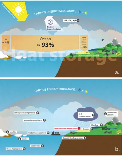
Earth’s Energy Imbalance (EEI). Because of EEI, the climate system stores energy. 93% of this energy warms the the ocean warming increasing the Ocean Heat Content (OHC), while the remaining 7% is responsible for the warming of the atmosphere and continents and ice melting [Levitus et al., 2012] (Fig. 1.6 top). EEI is responsible of the climate related changes in the Earth’s system, like the rise of the global-mean temperature (known as global warming), the rise of sea-level, the melting of glaciers, the changes in the global water cycle, etc. (Fig 1.6 bottom).

EEI can be estimated via: (1) direct measures by satellite using the Clouds and the

Earth’s Radiant Energy System (CERES)instruments, (2) directOHCestimation, via the

temperature measurements in the ocean from ARGO, and (3) indirect OHC estimation via the steric sea-level deduced from the GMSLR and the ocean mass through the sea level budget (Eq. 1.5).

The CERES instruments enable to retrieve EEI variations from weekly to decadal

timescales accurately with an uncertainty of ±0.1 W m−2 but the time-meanEEI is mea-sured with an accuracy of 3.0 W m−2 because of calibration issues [Loeb et al.,2012]. EEI

estimate is 0.71 ± 0.11 W m−2 for the period 2006 to 2015 [Meyssignac et al., 2019].

OHC deduced from ARGO data is computed from the ocean heat changes due to changes in temperature at each position and depth, integrated over the whole ocean. EEI

based on ARGO is 0.67 ± 0.17 W m−2 for the period from 2006 to 2015 [Meyssignac et al.,

2019]. This uncertainty is underestimated because it is estimated from the spread between the different solutions and do not include the sparseness of insitu data in critical areas as marginal seas, seasonally ice-covered regions and down to 6000 m depth [Meyssignac et al., 2019].

Indirect OHC deduced from the sea level budget presents the advantages of a global spatial coverage and integration over the whole column of water (from surface to sea floor). OHCderived from sea-level budget rely on sea-level, ocean mass and the expansion efficiency of heat (EEH) via Eq. 1.8. The expansion efficiency of heat is estimated about 0.12mY J−1[Levitus et al.,2012]. Sea-level budgetEEIis estimated at 0.69 ± 0.62 W m0−2

Figure 1.6: Schematic representations of the flow and storage of energy in the Earth’s climate system (top), and main consequences of the EEI in the Earth’s climate system (bottom)

[Llovel et al., 2014] and 0.48 ± 0.47 W m−2 [Meyssignac et al., 2019]. Uncertainty in EEI

estimated though the sea level budget is mainly due to the uncertainty in the ocean mass [Meyssignac et al., 2019].

OHC = EEH · GM SSLR = EEH · (GM SLR− ∆Mocean ρocean· Aocean

) (1.8)

EEI and the water cycle are related through the ocean mass via the sea-level budget and theOHC. We discuss the implications of the uncertainty in the ocean mass trends in the estimate ofEEI and its uncertainties in detail in Chapter 4.

1.5

Scientific questions associated to the water cycle

In summary, thanks to an unprecedented effort in the development of the observing systems in the last decades, the uncertainty in the estimation of the water cycle, the sea

budget at all timescales from annual to decadal within the uncertainties?

2. Are the uncertainty in the different components of the global water budget correlated when assessed with GRACE-based estimates?

3. Given the current uncertainty, can observed global water budget constraint climate models to reduce the spread in the 21st projections?

4. Given the current uncertainty, Are the causes of the recent acceleration in ocean mass increase significant and what is the cause?

5. Given the current uncertainty, has TWS increased or reduced the sea-level rise in the first decades of the 21th century? Why GRACE-based and model-based TWS

trends have opposite sign?

6. Given the current uncertainty, how is TWS changing under climate change? 7. Can we separate the glacier and the hydrology signals in space gravimetry signal?

Scientific questions related to the sea level budget

8. Can we close the sea level budget at annual and longer timescales under climate change, given the current uncertainties?

9. Is the deep ocean heating significant? What is its contribution to the steric sea level and to the EEI?

10. Can we reduce the uncertainty in the ocean mass estimate through the freshwater budget? Can we provide constraint?

11. Given the level of uncertainties, can we use ocean mass and geocentric sea-level observations with geodetic techniques to constrainEEI which is responsible for the contemporary climate change?

1.6

Objectives of this PhD

The scientific objectives are: (1) to document the nature of global mass exchanges with estimates and the associated uncertainties, and if we can, (2) explain the differences among

the estimates of the global water budget, (3) reconcile and propose robust estimates with uncertainties, (4) on this basis, reevaluate the estimates and revisit the scientific questions cited before and more specifically numbers 1 and 8.

To reach these scientific questions, I improve in my PhD work the treatment of space gravimetry data from GRACEto obtain consistent global mass changes with, as exhaus-tive as possible, associated uncertainties. I decided to use an ensemble approach including all available state-of-the-art post-processing to assess the underlying uncertainties.

The second chapter is focused on the development of an ensemble of GRACE solutions. I explain the state-of-the-art of the GRACE treatment and GRACE post processing. I explain how I developed a consistent ensemble of GRACE solutions that conserves mass at global scale. I explore the reason for differences between different GRACE solutions and provide some insights on the sources of the uncertainties in GRACE estimates of the global water cycle. I include a paper that discuss the uncertainties on the GRACE-based global water cycle [Blazquez et al.,2018]. At the end of the chapter, I compare the global water mass estimates with previous estimates, I explain the reason for the differences in previous estimates and I address questions: 1, 2, and 4.

In the third chapter, I focus on land, and I analyze the uncertainties in the land GRACE-based estimates at basin scale. I propose a method using independent mass estimates to reduce the uncertainties on the GRACE-based local water mass estimates. I test and validate this method in South Asia, a region where glaciers and lakes are concentrated in small locations. Accounting for their mass changes leads to improved estimate for other hydrological processes affecting the local water cycle. I summarize the method and validate the hydrological estimates inBlazquez et al.[2020, In prep], attached at the end. This provides regional insight on the science questions 6 and 7 and show the potential of using independent data to improve GRACE data and potentially respond to questions 5, 6, and 7 at global scale in the future, when the method will be applied to all regions influenced by glaciers and lakes.

In the fourth chapter, I focus on the ocean. I identify the geocenter motion correction and the GIAcorrection as the major sources of uncertainty in the ocean mass changes. I explore a method to improve the estimates of the ocean mass by removing the uncertainty in geocenter. I analyze the consistency between the ocean mass, the altimetry sea-level and the steric sea level through the sea-level budget. Thanks to the comparison with CERES-based steric sea-level, I identify the sources of some errors in GRACE-based ocean mass. I address questions 8, 9 and 10.

Evaluating the uncertainty in

GRACE-based estimates of the

global water budget. Development of

an ensemble approach

The main objective of this PhD is to characterize the global water budget at interan-nual to decadal timescales and to characterize the associated uncertainties. OnlyGravity

Recovery and Climate Experiment (GRACE)andGRACE FOmissions allow to estimate

at the same time all components of the global water budget at interannual to decadal time scales. A significant advantage of deriving estimates of all components from the same sin-gle mission is that all estimates, their errors, and their uncertainties should be consistent with each other by construction. For this reason, GRACE solutions have provided essen-tial and critical observations to analyze and test the closure of the global water budget [Church et al., 2013; Llovel et al., 2014; Yi et al., 2015; Reager et al., 2016; Rietbroek et al., 2016; Dieng et al., 2017]. However, in practice, there are significant differences in the water budget components estimates when different GRACE solutions from differ-ent data processing cdiffer-enters are used or when differdiffer-ent post-processing are applied to the data. So, each single post-processed GRACE solution provides a self consistent estimate of the global water budget components but this estimate is potentially biased. By self consistent, I mean that they close the global water budget. Thus, if GRACE solutions are considered with the same single post processing, they likely underestimate the true uncertainty in global water budget components.

I propose to estimate the components of the global water budget from GRACE and to evaluate the associated uncertainty using an ensemble of global GRACE solutions and an ensemble of post-processing parameters which includes all state-of-the-art GRACE solutions and post-processing parameters that are available. With this ensemble, I expect to capture most of the relevant state-of-the-art estimates of the global water budget from GRACE data. The range covered by my ensemble should enable to explore the uncertainty and to analyze its sources.

In this chapter, I present GRACE and GRACE FO missions in Section 2.1. I discuss the post-processing parameters used to produce GRACE solutions in Section2.2. I present