Pavement Distress Detection with Conventional Self-Driving
Car Sensors
by
Nizar TARABAY
THESIS PRESENTED TO ÉCOLE DE TECHNOLOGIE SUPÉRIEURE
IN PARTIAL FULFILLMENT OF A MASTER’S DEGREE
WITH THESIS IN ELECTRICAL ENGINEERING
M.A.Sc.
MONTREAL, OCTOBER 13, 2020
ÉCOLE DE TECHNOLOGIE SUPÉRIEURE
UNIVERSITÉ DU QUÉBEC
This Creative Commons license allows readers to download this work and share it with others as long as the author is credited. The content of this work cannot be modified in any way or used commercially.
BOARD OF EXAMINERS
THIS THESIS HAS BEEN EVALUATED BY THE FOLLOWING BOARD OF EXAMINERS:
Mr. Maarouf Saad, Thesis Supervisor
Department of Electrical Engineering, École de Technologie Supérieure
Mr. Gabriel Assaf, Thesis Co-supervisor
Department of Construction Engineering, École de Technologie Supérieure
Mr. Pierre-Jean Lagacé, President of the Board of Examiners
Department of Electrical Engineering, École de Technologie Supérieure
Mr. Chakib Tadj, Member of the jury
Department of Electrical Engineering, École de Technologie Supérieure
Mr. Imad Mougharbel, External member of the jury
Department of Electrical Engineering, École de Technologie Supérieure
THIS THESIS WAS PRESENTED AND DEFENDED
IN THE PRESENCE OF BOARD OF EXAMINERS AND THE PUBLIC ON SEPTEMBER 28, 2020
ACKNOWLEDGEMENTS
I would first like to express my deepest gratitude to my advisors Professor Maarouf Saad, Professor Gabriel Assaf, and Professor Imad Mougharbel for their guidance, help, and support through my research. This research would not be possible without their advice and feedback. I appreciate the time and effort they generously devoted to follow up on my work. Working with them is a real privilege and a great honour.
I would also like to thank my colleagues who work in the GREPCI Laboratory, the Electrical Engineering Department at École de Technologie Supérieure, GUS team, and the Technological Application Technicians in the Electrical Engineering Department for the technical and academic assistance.
I would also like to extend my appreciation to Professor Gabriel Assaf’s team, Nabil Agha, Marion Ghibaudo, and Valentin Marchioni, for their time, feedback, and help through all the stages of my project.
Thanks also to the jury members for taking the time to review and evaluate my work.
I would like to acknowledge Mitacs and WSP for their financial support and mentorship through Mitacs Acceleration Program.
I cannot express enough thanks to my parents, my sisters Jana and Rana, my brother Naji and my brother-in-law Rawad, my nephew Rani, and my friends for their support, love, and encouragement during my journey. I am grateful to have them in my life.
Détection de détérioration de chaussée avec des capteurs conventionnels de véhicule autonome
Nizar TARABAY RÉSUMÉ
Détecter et quantifier les détériorations des chaussées d’une façon adéquate est une tâche essentielle pour caractériser l’état des routes, identifier les causes de détérioration, développer des modèles de prévision de l’état futur, et quantifier les besoins en termes d’entretien et de réhabilitation à court et long termes. De nombreuses méthodes automatiques ont été développées pour détecter et évaluer les détériorations des chaussées. Cependant, ces méthodes font face à de nombreuses limitations telles que la fiabilité, la rentabilité, et le prix élevé. Par conséquent, elles ne sont pas fréquemment utilisées pour inspecter les routes. Dans ce projet, nous abordons ces limites en testant une nouvelle approche pour la collecte des données de surface des chaussées. Nous testons deux capteurs conventionnels installés sur les voitures autonomes, fixés sur un véhicule: Un LiDAR 3D, et un appareil photo RVB. La performance du LiDAR est validée via des mesures de sa capacité à détecter des dégradations. Les résultats montrent un écart entre les nuages de points acquis et ses références. La reconstruction de la surface à partir des nuages de points acquis montre des déformations significatives dans l’élévation de la chaussée. Cela est notamment dû aux bruits dans les mesures prises par le LiDAR, à sa faible précision qui se dégrade sur des surfaces moins réflectives, et à sa faible résolution.
D’autre part, l’appareil photo RVB montre de meilleurs résultats dans la détection des fissures routières. Dans ce projet, nous introduisons une approche complète pour les détecter. Nous utilisons une caméra pour enregistrer des vidéos tout en conduisant. Nous utilisons un algorithme d’apprentissage supervisé pour détecter les fissures. Nous adoptons une méthode originale pour annoter les images, que nous traitons ensuite avec un réseau de neurones à convolution pour sectionner les fissures. Nous validons le modèle sur 70 images. Les résultats montrent que la capacité de notre système pour la détection et segmentation de fissures est pertinente : la précision du modèle, une fois entraîné, est de 77,67 %, le rappel est de 79,18 %, et la moyenne de l’intersection sur l’union est 64.6%.
Mots-clés: Détection des détériorations des chaussées, Capteurs de véhicule autonome, LiDAR 3D, RVB camera, Réseau de neurones basé sur des régions, Mask R-CNN
Pavement distress detection with conventional self-driving car sensors Nizar TARABAY
ABSTRACT
Properly detecting asphalt pavement distresses before their expansion is a crucial task to characterize road condition in order to identify causes of deterioration and, therefore, maintain roads by selecting the appropriate intervention. Many automatic methods are developed to detect and assess pavement distresses. However, these methods face many limitations such as reliability, efficiency, and price. Hence, they are not frequently deployed for road inspections. In this project, we address those limitations by testing a new approach in collecting pavement data. We test self-driving car’s 3D LiDAR and RGB camera in detecting pavement distresses. We build our data acquisition platform and installed it on a moving vehicle. We conduct tests on the 3D LiDAR to assess its performance. Results show significant discrepancy between the scanned point cloud and its reference. Moreover, the reconstructed surface from the scanned point cloud shows significant deformations. This is mainly due to the noisy measurements, the low accuracy especially on low reflective surface, and the low resolution of the scanned point cloud.
On the other hand, RGB camera shows a better performance in detecting cracks. We introduce a full approach for crack detection. We use a non-expensive camera to collect data on a moving vehicle. We use a supervised learning algorithm to detect cracks. We adopt an original way in annotating the collected dataset. Finally, we process it with a region-based deep convolutional neural network for instance segmentation. We validate the trained model on 70 images, rich with different scenarios, crack shapes, and noises, collected from a moving vehicle with a low-cost camera. Results show the capacity of our approach in crack detection and segmentation. The precision of the trained model is 77.67%, its recall is 79.18%, and the average intersection over union is 64.6%.
Keywords: Pavement distress detection, Autonomous vehicle sensors, 3D LiDAR, RGB camera, Regional Based Neural Network, Mask R-CNN
TABLE OF CONTENTS
Page
INTRODUCTION ...1
CHAPTER 1 BACKGROUND AND RELATED WORK ...5
1.1 Pavement and Distress Types ...5
1.1.1 Pavement with Asphalt Concrete Surface ... 6
1.1.2 Pavement with Jointed Portland Cement Concrete Surface ... 7
1.1.3 Pavement with Continuously Reinforced Concrete Surface ... 9
1.2 Manual Inspection ...11
1.3 Automated Inspection ...12
1.3.1 2D Image Processing ... 13
1.3.2 3D Based Reconstruction Method ... 16
CHAPTER 2 SELF-DRIVING CAR SENSORS AND HARDWARE CONFIGURATION ...21
2.1 Self-Driving Car Sensors ...21
2.1.1 LiDARs ... 21
2.1.2 RGB Camera ... 23
2.2 Motivation ...23
2.3 The Hardware Setup ...23
2.3.1 LiDAR Selection ... 24
2.3.2 LiDAR Scanning Visualization ... 25
2.3.3 2D Camera Selection ... 28
2.3.4 Data Processing ... 29
2.3.5 Hardware Configuration ... 30
CHAPTER 3 SELF-DRIVING CAR’S SENSORS: TESTS AND RESULTS ...33
3.1 Experiments on the LiDAR ...33
3.1.1 Indoor Experiments ... 34
3.1.1.1 Cloud to Cloud/Mesh Distance ... 34
3.1.1.2 Results Interpretation ... 43
3.1.1.3 Screened Poisson Surface Reconstruction ... 44
3.1.1.4 Results Interpretation ... 46
3.1.2 Outdoor Experiments ... 46
3.1.2.1 Depth Information from the Reconstructed Surface ... 48
3.1.2.2 Results Interpretation ... 53
3.1.3 Conclusion ... 53
3.2 RGB Camera ...53
3.2.1 Object Detection and Instance Segmentation with RPN ... 54
3.2.1.1 Regions with Convolutional Neural Network (R-CNN) ... 54
3.2.1.2 Fast R-CNN ... 55
3.2.1.4 Mask R-CNN ... 59
3.2.2 Mask R-CNN in Detecting Cracks: Experiments and Results ... 70
3.2.2.1 Training and Validating the Results on Mask R-CNN ... 73
3.2.3 Conclusion ... 86
CONCLUSION AND RECOMMENDATION ...89
ANNEX I ACQUIRING THE LIDAR DATA ...93
ANNEX II LIDAR CHANNEL ANGLES ...95
ANNEX III THE READABLE FORMAT FILE ...97
ANNEX IV MASK R-CNN CONFIGURATION ...99
ANNEX V PREPARING THE DATASET, TRAINING AND EVALUATING MASK R_CNN ...101
LIST OF TABLES
Page
Table 1.1 ACP distress types ...7
Table 1.2 JCP distress types ...9
Table 1.3 CRCP distress types ...10
Table 2.1 LCMS and Ouster OS-1 specifications ...22
Table 2.2 Velodyne and Ouster LiDARs specifications and prices ...25
LIST OF FIGURES
Page
Figure 1.1 JCP Cross section ...8
Figure 2.1 Ouster-128 channels LiDAR mounted horizontally ...26
Figure 2.2 Ouster-128 channels LiDAR directed downward ...26
Figure 2.3 Ouster-64 channels LiDAR directed downward ...27
Figure 2.4 Ouster-16 channels LiDAR directed downward ...27
Figure 2.5 The LiDAR and the camera installed on the top of the car ...31
Figure 3.1 Environment 2, surface with mixed reflectivity ...35
Figure 3.2 Environment 1, high reflectivity point cloud ...36
Figure 3.3 Environment 2, mixed reflectivity point cloud ...36
Figure 3.4 Reference point cloud ...37
Figure 3.5 Cloud to cloud distance ...38
Figure 3.6 Cloud to Cloud distance. High reflectivity surface compared to its reference point cloud ...39
Figure 3.7 Histogram of the absolute distance between the scanned point cloud (high-reflectivity surface) and its reference ...39
Figure 3.8 Cloud to Cloud distance. Chess board compared to its reference point cloud ...40
Figure 3.9 Histogram of the absolute distance between the scanned point cloud (mixed-reflectivity surface) and its point cloud reference ...40
Figure 3.10 Cloud to mesh distance. High-reflectivity surface ...41
Figure 3.11 Histogram of the absolute distance between the scanned point cloud (high-reflectivity surface) and its plane reference ...42
Figure 3.12 Cloud to mesh distance. Mixed-reflectivity surface ...42
Figure 3.13 Histogram of the signed distance between the scanned point cloud (mixed-reflectivity surface) and its reference ...43
Figure 3.15 Reconstructed map of the high-reflective surface ...45
Figure 3.16 Reconstructed map of the mixed-reflective surface ...46
Figure 3.17 RGB frame with its equivalent ambient LiDAR data ...47
Figure 3.18 RGB frame with its equivalent reflectivity LiDAR data ...48
Figure 3.19 RGB frame and its LiDAR equivalent; pavement with no depth deformation ...49
Figure 3.20 Pavement reconstruction with faulty depth deformation ...49
Figure 3.21 RGB frame and its LiDAR equivalent; pavement with a low severity pothole...50
Figure 3.22 Pavement reconstruction with low severity pothole, the blue and red areas are faulty detections ...51
Figure 3.23 RGB frame and its LiDAR equivalent; pavement with high severity pothole...52
Figure 3.24 Pavement reconstruction with high severity pothole ...52
Figure 3.25 R-CNN model architecture ...55
Figure 3.26 Fast R-CNN architecture...56
Figure 3.27 Faster R-CNN architecture ...58
Figure 3.28 Prediction at different feature layers ...59
Figure 3.29 Residual block ...60
Figure 3.30 FPN diagram ...61
Figure 3.31 RPN diagram showing the two classification and the bounding boxes branches ...62
Figure 3.32 Intersection over Union ...64
Figure 3.33 Box head feature extraction ...66
Figure 3.34 2 x 2 ROI max pooling...67
Figure 3.35 Bilinear interpolation in RoIAlign ...68
Figure 3.37 Mask R-CNN block diagram ...70
Figure 3.38 The conventional pipeline used for supervised machine learning algorithms ...71
Figure 3.39 RGB image (left) and its corresponding ground truth (right). Different colours refer to different fractions of the crack, each colour in the GT image is considered as a separate object ...72
Figure 3.40 Cracks in different lighting conditions, with random objects and different pavement materials ...73
Figure 3.41 Architecture of Mask R-CNN ...74
Figure 3.42 From left to right: RGB image with the GT; the top 40 mini proposals generated by ROI network; and the segmentation ...75
Figure 3.43 From left to right: RGB image with the GT; crack segmentation before applying the merge function; and after applying the merge function ...76
Figure 3.44 Top 150 proposals with their confidence scores ...77
Figure 3.45 Final detection, before refinement (dotted lines), after refinement (solid lines)...77
Figure 3.46 The final mask detection ...78
Figure 3.47 A selection of the C2 feature maps output ...79
Figure 3.48 A selection of the C3 feature maps output ...79
Figure 3.49 A selection of the C4 feature maps output ...80
Figure 3.50 A selection of the C5 feature maps output ...80
Figure 3.51 Alligator crack segmentation. Left: Ground truth segmentation. Middle: bounding box detection. Right: mask segmentation ...82
Figure 3.52 Low noise crack segmentation. Left to right columns: RGB image; GT; mask segmentation ...84
Figure 3.53 Moderate noise crack segmentation. Left to right columns: RGB image; GT; mask segmentation ...85
Figure 3.54 High noise crack segmentation. Left to right columns: RGB image; GT; mask segmentation ...86
LIST OF ABREVIATIONS 1D 1 Dimensions
2D 2 Dimensions 3D 3 Dimensions
LiDAR Light Detection And Ranging DIM Distress Identification Manual LTPP Long-Term Pavement Performance ACP Asphalt Concrete-surface Pavement
JCP Jointed Portland cement concrete-surfaced pavement PCC Portland Cement Concrete
CRCP Continuously Reinforced Concrete Pavement PCI Pavement Condition Index
DNN Deep Neural Network
CNN Convolutional Neural Network HNE Holistically-Nested Edge
FPHBN Feature Pyramid Hierarchical Boosting Network RGB-D Red Green Blue Depth
GNSS Global Navigation Satellite System IMU Inertial Measurement Unit
DMI Distance Measuring Instrument MLS Mobile Laser Scanner
LCMS Laser Crack Measurement System IT Information Technology
FoV Field of View
ADAS Advanced Driver-Assistance Systems USD United States Dollar
GPU Graphic Processing Units C2C Cloud to Cloud
C2M Cloud to Mesh
R-CNN Region Convolutional Neural Network mAP Mean Average Precision
FC Fully Connected RoI Region of Interest
RPN Region Proposal Network FPN Feature Pyramid Network COCO Common Objects in Context GT Ground Truth
TP True Positive FP False Positive
AIU Average Intersection over Union
M Million
BB Bounding Box
NMS Non Maximum Suppression FCN Fully Convolutional Network CCE Categorical Cross Entropy
BCE Binary Cross Entropy CE Cross Entropy
FHWA Federal Highway Administration CFD CrackForest Dataset
IOU Intersection Over Union HD High Definition
SFF Shape from Focus SFDF Shape from Defocus
LIST OF SYMBOLS φ LiDAR angle with an horizontal plane
d LiDAR height to the ground
δ Channels’ direction angle inside the LiDAR θ Laser beam firing angle
r LiDAR range
LIST OF MEASUREMENT UNITS
s Second (time unit)
m Meter (length unit)
mm Millimeter (length unit) cm Centimeter (length unit)
Km/h Kilometer per hour (speed unit)
Hz Hertz (frequency unit)
INTRODUCTION
Pavement distresses substantially impact the driving comfort, the vehicle operating costs and the road safety. The main causes of pavement distresses are: poor construction, fatigue due to heavy traffic, and natural factors such as water action and extreme temperature fluctuations. A reliable pavement distress detection tool would help to collect efficiently pavement distress data, to characterize road conditions and to identify the causes of pavement deterioration. The diagnostic of the causes of pavement deterioration is needed to select the appropriate intervention by solving the source of the problem rather than applying an inadequate treatment which will deteriorate rapidly.
Conventional assessment methods such as visual inspections, 2D computer vision methods, and 3D reconstruction methods, can detect pavement distresses and evaluate the pavement quality. Nevertheless, these methods are time-consuming and expensive, and may be inefficient especially in cities where road network is dense and subject to high volume traffic. Therefore, finding an effective tool to detect and classify pavement distress, such as deformation and cracks, is crucial to maintain roads in good condition, reduce user costs, and improve traffic safety.
Many inspection methods for pavement distress detection and classification are developed for commercial use. These methods fall in two categories: automated inspection and manual inspection. Automated methods rely on special equipment to detect pavement distresses. For instance, cameras are used to detect distresses such as cracks, potholes, and patches.However, cameras are not suitable to detect polished aggregate, raveling, and water bleeding. 3D sensors are more suitable to detect almost all distresses. Other sensors are also deployed to detect pavement distresses. For instance, accelerometer, microphone, sonar, and pressure sensors are used. However, these sensors are limited to specific types of distresses.
2D images taken by a camera and 3D images taken by 3D sensors, alongside the manual methods, are the common methods used in the detection of pavement distresses. Nevertheless, these three techniques face several limitations related to their efficiency, reliability, and price. Therefore, researchers are constantly trying to overcome those limitations by developing an efficient, reliable, and a low-cost pavement distress detection tool.
In this research, we address the aforementioned limitations by testing a low-cost solution based on 2D and 3D imagery to detect pavement distresses. We expect that this solution is more convenient by adopting onboard self-driving car sensors. And since self-driving cars are expected to be widely used in the future, exploiting their onboard technologies to assess road conditions may simplify the pavement data collection process, reduce its associate costs, allow to collect more data and therefore, improve the pavement inspection service. Furthermore, using the onboard self-driving cars’ sensors for pavement distress detection eliminates the need for a dedicated external and expensive equipment to evaluate the pavement conditions.
Self-driving cars adopt multiple sensing technologies to map the surrounding environment, these technologies use a Light Detecting and Ranging, also known as LiDARs, radio detection and ranging, radars, cameras, and ultrasonic sensors in addition to other different sensors. This research focuses on using the two main vision sensing components of self-driving cars: 3D LiDAR technology and 2D camera.
Self-driving car’s vision sensors are dedicated for obstacle detection and object recognition. To use these sensors for road condition assessment activity, their performance in detecting pavement distress has to be tested and validated. Thus, in this research, we address the following problematics:
• are the conventional self-driving car’s 3D LiDAR and camera convenient for pavement distress detection?
• what are the limitations of the 3D LiDAR and of the camera in pavement assessment application and what are the methods to overcome the limitations?
• is the pavement distress detection tool, based on self-driving car’s sensors, feasible to be deployed on current cars equipped with the adequate sensors?
To answer the above questions, we conduct several experiments inside the laboratory and in a real environment with a 3D LiDAR, similar to the one used in autonomous vehicles, and a 2D camera. We install the two sensors on a car and we drive on arterial roads in Montreal City. With the LiDAR, we collect the surrounding point cloud from which 3D points that belong to the pavement surface are extracted. With the camera, we capture the pavement surface. We test the extracted data to validate the capacity of both the 3D LiDAR and the camera in detecting pavement distresses.
The remainder of this report is organized as follows:
In chapter 1, we present the research background and the relevant literature review. First, we introduce the different types of pavements and associated types of surface deterioration that affect them. Next, we present the different methods to measure and assess the different types of pavement distress. Then, we present a critical review of the current methods deployed on the market and developed by researchers to detect pavement distress, highlighting advantages and limitations of each method.
In chapter 2, we present the motivation, the challenges, and the approach adopted to tackle the research problematics. First, we show the current self-driving car sensing technologies, then, we present the equipment used in this research for data collection.
In chapter 3, we show the experiments conducted on the LiDAR and the camera. We conduct experiments inside the laboratory and experiments in a real environment to test the capacity of the 3D LiDAR in detecting deformations on road surface. We address reliability, effectiveness, and price limitations of the state-of-the-art 2D image-based methods by introducing a complete
approach for crack detection. We present the adopted machine learning algorithms and test it in detecting cracks. Finally, we discuss the results of the tests.
In the final section, we summarise and conclude our research, and propose recommendations for future works.
CHAPTER 1
BACKGROUND AND RELATED WORK
Designing durable road networks is a challenge for construction engineers. Different techniques, construction materials, and mixes are available to enhance the quality of the pavement and reduce its susceptibility to deteriorate under heavy traffic or climate conditions. However, pavements, regardless their composition, tend to deteriorate and require a periodic inspection and preventive maintenance. Therefore, several pavement inspection methods had been developed to characterize road condition. Chapter 1 addresses the different types of pavement surfaces and their specific distresses. It also reviews the current manual and automated pavement surface distress detection methods. Chapter 1 is divided into three sections. In Section 1.1, we show common types of pavement surfaces, and distresses that can affect them. In Sections 1.2 and 1.3, we review the measurement and assessment tool, and the current methods for pavement distress detection (i.e., manual and automated inspection).
1.1 Pavement and Distress Types
Construction engineers study different factors while designing or rehabilitating roads. The cost and the lifetime of the used materials, the maintenance cost, the traffic volume, and the climatic conditions are some of these factors. The Distress Identification Manual (DIM) for the Long-Term Pavement Performance Program (LTPP) (Miller & Bellinger, 2014), inspect pavement distresses on three different types of pavements: (1) pavements with asphalt concrete surfaces, (2) pavements with jointed Portland cement concrete surfaces, and (3) pavements with continuously reinforced concrete surfaces. In the following section, we briefly present the aforementioned types of pavements and what distresses are prone to develop on each, according to the LTPP Manual.
1.1.1 Pavement with Asphalt Concrete Surface
Asphalt Concrete-surface Pavement (ACP) is a common type of roads. Since the beginning of the twentieth century, road construction engineers use ACP (Polaczyk et al., 2019), which has relatively low-cost materials and it is easy to maintain compared to other pavements surfaces; however, it is considered as the less environmental friendly among the other common pavement surfaces. According to LTPP, ACP is susceptible to 15 different distress types that fall into five categories:
1. Cracking - Many possible reasons lead to different types of cracking, mainly fatigue in the asphalt surface under high traffic load, or harsh weather conditions;
2. Patching and potholes - Patching: a road area covered with new materials. Potholes: Depressions in the surface characterized by their depth and their area;
3. Surface deformation - Grooves on the wheel path caused by the high traffic load, overweight vehicles, or a failure in the pavement construction material;
4. Surface defects - Bleeding: It occurs when the asphalt binder expel through the aggregate due to high temperature. A bleeding surface may be characterized by its shiny, reflective surface, its fading texture and surface discolouring. Polished aggregate: the aggregate level above the asphalt surface starts to erode. Ravelling is characterized by the loss of surface aggregate;
5. Miscellaneous distresses - Lane to shoulder drop off: a drop off in the level of the road between the lane and the shoulder. Water bleeding: water leaks from joints or cracks.
Table 1.1 summarises all the different types. Each type has a unique description, severity levels, and unique measurement methods. For instance, fatigue cracking is labelled according to its severity level (i.e., low, moderate, and high) and measured by the surface of the affected area. Potholes, on the other hand, are measured by their surface and their depth.
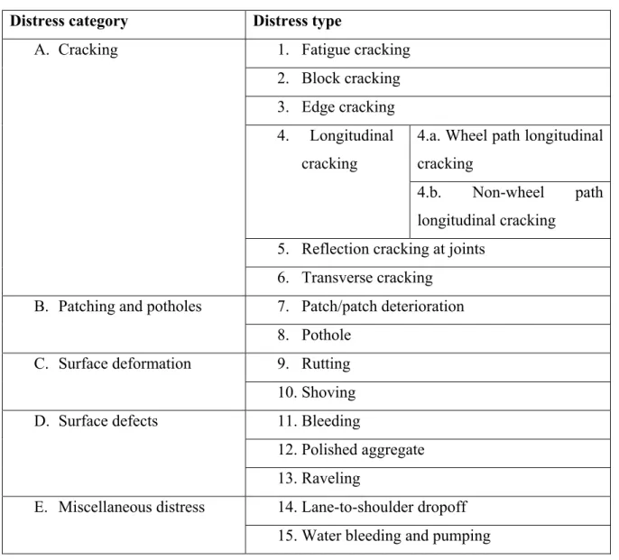
Table 1.1 ACP distress types Adapted from Miller et Bellinger (2014) Distress category Distress type
A. Cracking 1. Fatigue cracking 2. Block cracking 3. Edge cracking 4. Longitudinal
cracking
4.a. Wheel path longitudinal cracking
4.b. Non-wheel path longitudinal cracking
5. Reflection cracking at joints 6. Transverse cracking
B. Patching and potholes 7. Patch/patch deterioration 8. Pothole
C. Surface deformation 9. Rutting 10. Shoving D. Surface defects 11. Bleeding
12. Polished aggregate 13. Raveling
E. Miscellaneous distress 14. Lane-to-shoulder dropoff 15. Water bleeding and pumping
1.1.2 Pavement with Jointed Portland Cement Concrete Surface
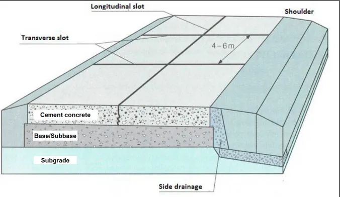
Jointed Portland cement concrete-surfaced pavement, or JCP, is another popular choice for road construction. JCP is composed of Portland cement concrete (PCC) constructed on top of the subgrade or the base course. Figure 1.1 (Szymański et al., 2017) shows a cross section of a JCP. JCP is known for its strong characteristics, the low-cost maintenance, the capacity of load
carrying, and its long life span. However, the initial cost of the JCP construction is high, and it is subject to crack and warp in harsh weather and high temperature fluctuations (Sautya, 2018).
Figure 1.1 JCP Cross section Adapted from Szymański et al. (2017)
LTPP manual groups the different types of JCP distress into four different categories: (1) cracking, (2) joint deficiencies (i.e. deficiencies between the concrete slabs), (3) surface defects, and (4) miscellaneous distresses. Table 1.2 summarizes the different types of JCP distresses.
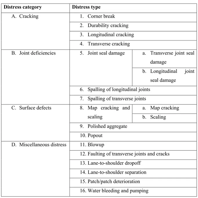
Table 1.2 JCP distress types Adapted from Miller et Bellinger (2014) Distress category Distress type
A. Cracking 1. Corner break 2. Durability cracking 3. Longitudinal cracking 4. Transverse cracking
B. Joint deficiencies 5. Joint seal damage a. Transverse joint seal damage
b. Longitudinal joint seal damage
6. Spalling of longitudinal joints 7. Spalling of transverse joints C. Surface defects 8. Map cracking and
scaling
a. Map cracking b. Scaling 9. Polished aggregate
10. Popout D. Miscellaneous distress 11. Blowup
12. Faulting of transverse joints and cracks 13. Lane-to-shoulder dropoff
14. Lane-to-shoulder separation 15. Patch/patch deterioration 16. Water bleeding and pumping
1.1.3 Pavement with Continuously Reinforced Concrete Surface
Continuously reinforced concrete pavement or CRCP is another type of pavements that has a long-term service life under harsh environmental conditions, temperature fluctuations, and
heavy traffic (Tyson & Tayabji, 2012). CRCP has no joints, it’s a single rigid construction reinforced with steel bars. A well-performing CRCP has a uniform transversal crack pattern. The uniform crack pattern reflects the consistency of the concrete mixture (Tyson & Tayabji, 2012). LTPP categorize CRCP distresses into three categories: (1) cracking, (2) surface defects, and (3) Miscellaneous distresses. Table 1.3 lists the different types of CRCP distress.
Table 1.3 CRCP distress types Adapted from Miller et Bellinger (2014) Distress category Distress type
A. Cracking 1. Durability cracking 2. Longitudinal cracking 3. Transverse cracking
B. Surface defects 4. Map cracking
and scaling
c. Map cracking d. Scaling 5. Polished aggregate
6. Popout C. Miscellaneous distress 7. Blowup
8. Transverse construction joint deterioration
9. Lane-to-shoulder dropoff 10. Lane-to-shoulder separation 11. Patch/patch deterioration 12. Punchout
13. Spalling of longitudinal joints 14. Water bleeding and pumping 15. Longitudinal joint seal damage
We should also mention that unpaved/dirt road is another type of pavement construction. It is mainly built in rural areas with harsh climate and temperature below freezing where the other pavement types fail or need a frequent maintenance.
1.2 Manual Inspection
Collecting pavement distress data is a crucial task to maintain roads and assess their condition. Different researchers and organizations develop distress catalogues that provide descriptions and methods for measuring pavement distresses and quantify their severity level. For instance, the Distress Identification Manual for the Long-Term Pavement Performance Program (LTPP Manual) developed by the US Department of Transportation, targeting United States and Canada road networks, offers a consistent method for a manual distress data collection (Miller & Bellinger, 2014; Ragnoli et al., 2018). ASTMD-6433 (D6433-18, 2018) also provides a standardization to identify and classify pavement distresses. It quantifies the pavement conditions with visual surveys using the Pavement Condition Index (PCI). In Europe, standards on distress identification and management are limited to the French Institute of Science and Technology for Transport, the Swiss Association of Road and Transport Professionals, and studies in Ireland to evaluate the surface of the pavement (Ragnoli et al., 2018).
Manual inspection methods consist of conducting a visual inspection or road surveys. By evaluating the road while driving, the inspectors report distress conditions according to their severity, density, and type. They also report the smoothness and ride comfort of the road. Visual inspection typically measures the Pavement Condition Index: an index of 100 reflects the best road condition and a zero index reflects the worst. This method is widely used due to its simplicity, but it does not return accurate information on the road distress (e.g., dimension and number of the encountered distress). It is also considered as a subjective evaluation method that depends on the inspector’s experience and capability of accurately detecting all types of pavement distress.
Another manual method consists in conducting surveys. For instance, LTPP Manual introduces a survey method that consists in building a distress map showing the pavement distress location and severity level by walking or driving while searching for surface defects.
Manual methods are considered as a slow road inspection process, labour intensive, and may expose the workers and the driver safety to serious risks. They are also susceptible for human subjectivity and errors. And since obtaining the right distress information from the road is crucial for accurate surveys, service providers and researchers highly invest in developing the right technologies and in training the staff for the manual inspection (Ragnoli et al., 2018).
1.3 Automated Inspection
Due to the several limitations of manual inspection methods, researchers and service providers develop many systems to automate the process of collecting pavement distress data and to provide a non-subjective, more efficient, and accurate data. The automated inspection methods are based on quantifying each pavement distress. These methods often measure the width, the depth, the severity level, the road elevation, and classify distresses according to their types.
Automated methods offer more options in detecting road deteriorations. According to (Coenen & Golroo, 2017) and (Kim & Ryu, 2014), automated techniques can be classified into different categories: (1) Vision based method including 2D images and/or video processing, (2) 3D reconstruction method based on 3D sensor, (3) vibration-based method including accelerometer, microphone, and pressure sensors that reacts to the vibration force resulted from road deformation. These methods differ by the detection equipment and the type of road deterioration that they detect. For instance, the vision-based method and the 3D reconstruction methods have the highest amount of distress detection, hence, they are commonly used by pavement inspection service providers.
1.3.1 2D Image Processing
2D image processing methods are based on collecting road images with a moving or stationary camera. A moving data acquisition platform requires a high-speed and high-definition camera mounted on an inspection vehicle. This method allows inspectors to collect data while driving at a high speed. While this method provides high-quality images, it is expensive to be deployed on multiple cars. Moreover, collecting pavement data with a low number of equipped cars is inefficient especially while scanning a large road network. On the other hand, collecting still images is not an effective method since it is time-consuming, and it adds human interference at each distress location.
Following the data collection phase, 2D image processing algorithms are used to detect distresses. Oliveira et Correia (2014) develop a toolbox, CrackIT, to detect and classify cracks. The toolbox is based on four modules: (1) image preprocessing (e.g., image smoothing, white lane detection, etc.), (2) crack detection with pattern recognition techniques, (3) crack classification into types, and (4) evaluation routines to evaluate results (i.e., precision, recall, and Fm metrics). As reported in Oliveira et al. paper, CrackIT toolbox algorithms achieve a precision of 95.5% and a recall of 98.4%.
The CrackTree method is another crack detection method developed by Zou et al. (2012). The authors address the low contrast problem between cracks and the surrounding pixels (i.e., the shadow problem). The CrackTree method achieves a 79% precision and a 92% recall. However, CrackIT and CrackTree methods did not address the generalization problem: detecting cracks from images collected with moving vehicles and from images with different intensity, luminosity, blurring, and noise levels. Moreover, Koch et al. (2015) in their review on computer vision-based detection methods, list the limitations of such methods. The authors mention that the generalization is still a problem for the classic computer vision-based methods.
Akagic et al. (2018) work on an unsupervised method for detecting pavement crack using Otsu thresholding. The authors in their work split the developed method into two phases. In the first phase, the authors split their image into four small images. They calculate the mean and standard deviation for each small image. In the second phase, they calculate the image histogram and the Otsu thresholding. Otsu thresholding is a method to find an adaptive threshold that binarize the image into two classes: a background and a foreground. This is done by finding the values of the within-class variance and the between-class variance of an image. According to Akagic et al. (2018) the Otsu thresholding method achieves 77.77% recall and 77.27% precision on their own 50 images dataset. The authors reported that unwanted noise in the background can result after applying the Otsu thresholding. Moreover, we noticed that the segmented cracks miss a significant number of pixels that should be considered as a crack object. This is due to the difference in the luminosity level and the colour contrasts in a crack.
Classic computer vision methods highly depend on illumination and weather conditions, even shadows may affect the results of pavement distress extraction, these methods may return faulty detection results and/or fail to detect others. In addition, the lack of exact geospatial tagging for each image and the image distortion may also affect the accuracy and the efficiency of this method (Guan et al., 2016).
More recent works in computer vision-based methods focus on crack detection using supervised machine learning techniques. L. Zhang et al. (2016) apply Deep Neural Network model, DNN, to detect cracks. They train their model with 500 still images collected with a smartphone. They achieve a precision of 87% and a recall of 92.5% on their own-collected dataset. Furthermore, the authors reported that Convolutional Neural Network (CNN) provides superior crack detection performance compared to handcraft feature extraction methods. The results in (L. Zhang et al., 2016) are reported on crack patches with 99 × 99 pixels in size.
Gopalakrishnan et al. (2017) use DNN with transfer learning to detect cracks in 212 images from the Federal Highway Administration (FHWA) and LTPP database. The authors use
VGG-16 (Simonyan & Zisserman, 2014), a deep convolutional neural network pre-trained on the massive ImageNet database (Deng et al., 2009). They use the first 15 layers of this network as a feature generator network to extract features from 760 images. Then, they use the extracted features to train another classifier to categorize crack and non-crack images. The highest accuracy reported in this paper is about 90% for VGG-16 followed by a neural network classifier. Gopalakrishnan et al. experiment with crack/non-crack classification but they did not address the detection nor the segmentation challenge. Furthermore, the authors in (Alfarrarjeh et al., 2018) use region-based deep learning approaches for road damage detection. Alfarrarjeh et al. (2018) report a 62% F1 score (F1 score corresponding to a weighted average of precision and recall) while detecting bounding boxes around the damaged road area. Gopalakrishnan et al. (2017) and Alfarrarjeh et al. (2018) did not report scores on crack segmentation.
Attard et al. (2019) use Mask Regional Convolutional Neural Network or Mask R-CNN, which is a DNN for object detection (He et al., 2017), to detect cracks on concrete wall surfaces. They report a 93.94% precision and a 77.5% recall. They prove that Mask R-CNN can be used for detecting cracks. However, their research is based on still images for concrete walls and not for concrete or asphalt pavement surface. Mask R-CNN is a multi-stage deep neural network for object detection and segmentation. It uses ResNet (Kaiming He et al., 2016) to generate feature maps. It also uses the feature pyramid network architecture (Lin et al., 2017) to preserve the semantic values in the feature map from the deep convolutional layer and the resolution from the first convolutional layers. For the pixel wise detection or the segmentation task, Mask R-CNN uses a fully convolutional networks (Long et al., 2015). More details on Mask R-CNN architecture is presented in Chapter 3.
A recent work by Yang et al. (2019), report a maximum F1 score equal to 60.4% on the CRACK500 dataset (L. Zhang et al., 2016) and 68.3% on the CrackForest Dataset, CFD dataset, (Shi et al., 2016). Their method is based on feature pyramid method (Lin et al., 2017). The authors in (Yang et al., 2019) adopt the Holistically-Nested Edge (HNE) method (Xie &
Tu, 2015). According to Yang et al. (2019), crack detection task is very similar to the edge detection task since they share common features. The Feature Pyramid Hierarchical Boosting Network (FPHBN), (Yang et al., 2019), achieves the best results on different datasets (whether for CRACK500, Cracktree200, CFD, GAPs384 (Eisenbach et al., 2017), Aigle-RN (Amhaz et al., 2016)) compared to the other state-of-the-art methods.
1.3.2 3D Based Reconstruction Method
The reconstruction method based on 3D sensor can be divided into different categories: (1) visualization using Microsoft Kinect sensor, (2) stereo vision, (3) 3D laser scanner, (4) shape from focus and defocus (SFF, SFDF), and (4) photometric stereo method. The first method is based on Microsoft Kinect sensor which is a low-cost infrared, Red Green Blue – Depth, (RGB-D), camera. Microsoft Kinect is mainly used in gaming and robotics application. Joubert et al. (2011) and Moazzam et al. (2013) respectively, investigate the detection of potholes using a Kinect sensor. Y. Zhang et al. (2018) also investigate the Kinect sensor on a fixed platform; the acquired results from the three references show its potential in pavement inspection. However, Kinect sensor visualization is susceptible to infrared saturation when it is directly exposed to the sun light (Abbas & Muhammad, 2012). Moreover, this method needs further research and development in terms of detecting different types of pavement distress, integrating the Kinect sensor with different sensors (e.g., Global Navigation Satellite Systems (GNSS), Inertial Measurement Unit (IMU), and Distance-Measuring Instruments (DMI)), deploying the entire system on a moving platform, and performance validation in a real environment.
Stereo vision method captures 3D images by using two 2D cameras and epipolar geometry. To build a 3D surface, a spatial relationship based on epipolar geometry is established between points from the two 2D images. This technique faces several limitations such as motion blur, object occlusion, and needs sophisticated equipment. According to Mathavan et al. (2015), this
method is only suitable to detect potholes and rutting. Compared to 3D laser scanners, stereo vision method has limited types of pavement distress detection.
Shape from focus (SFF) method consists of computing the depth by measuring the circle of confusion of a point in the captured image. When an object in the captured image is not in the range of the camera focus it will appear blurred. Once the object in-focus, the distance of the object from the camera is computed. Algorithms such as Tenengrad (W. Huang & Jing, 2007), (Sun et al., 2005) and the modified Laplacian (Nayar & Nakagawa, 1994) are used to compute the distance of an object in an image. This method is hard to implement on a moving vehicle due to the need of taking multiple images from different optical axis positions from a stationary device (Mathavan et al., 2015). This method is only suitable to capture macro or micro texture from a standstill device (Mathavan et al., 2015)
Shape from defocus (SFDF) method uses special algorithm, e.g. zero-mean Gaussian depth-defocus (Kuhl et al., 2006), to compute the distance from a camera by measuring the amount of blurring or defocusing in an image, in contrast to SFF method, SFDF requires fewer images (Subbarao & Surya, 1994).
Photometric stereo is another method that consists of taking multiple image of the same object from a stationary camera while exposing the captured scene to different light sources. This method can only be used with special equipment and from a stationary devise.
3D laser methods can be extended to detect different types of pavement distress with high precision and accuracy. 3D laser scanner has undergone intense study since it is capable to acquire an enormous accurate number of data at a high rate; the collected data are called point cloud. The larger the number of acquired points is, the denser the point cloud is. Each point belonging to the point cloud mainly has a 3D coordinate and a geotagging reference. Three types of navigation sensors involve in referencing these points: (1) a Global Navigation Satellite System (GNSS), (2) an Inertial Measurement Unit (IMU), and (3) Distance
Measurement Instrument (DMI). All these components besides a 3D laser scanner(s), camera(s), and a control unit are mounted on a moving platform (mainly on a moving vehicle in road inventory) form a Mobile Laser Scanner (MLS) or land-based, which is also known as mobile LiDAR (Light Detection And Ranging) (Guan et al., 2016). According to Coenen et Golroo (2017) and Mathavan et al. (2015), MLS in pavement inspection is usually used to detect cracks, potholes, rutting, patching, bleeding, macro texture, shoving, raveling, joint faulting, and spalling.
Another method based on laser scanner technology is used in pavement inspection. This method is called a high-resolution 3D line laser scanner. This technology is deployed and commercialized by several companies such as “ROMDAS,” “Arrb group,” “Mandli communications,” etc. These companies collect high-resolution data for road profile by using a Laser Crack Measurement System (LCMS) developed by “Pavemetrics” (ROMDAS, 2016). Laurent et al. (2018) address this technology in their article. According to Laurent et al. two laser profilers are used to cover up to 4-meter road lane profile. 4,000 3D points are acquired for each profile to form a 3D transverse profile. The profile rates of line laser scanner sensors can attend a frequency up to 28,000 Hz allowing a longitudinal resolution of 1 mm at vehicle speed of 100 km/h (Laurent et al., 2018). This high resolution and high accuracy system detects different pavement distresses, and even analyses surface texture.
Many different techniques are used in calculating the depth of pavement distress by the 3D laser scanner method. The triangulation method is mainly used in line laser scanner; phase-shift and time of flight are mainly used in LiDAR technology. The triangulation technique is the fastest and most accurate and precise technique, followed by the phase shift, and finally the time of flight. For this reason, the line laser scanner has been adopted by many companies to detect pavement profiles at a high resolution and a high speed. However, the LiDAR technology is mainly employed in road inventory, to build a complete 3D model of roads and its elements (e.g., vehicles, pedestrian, pavement, joints, trees, building, road, signs, etc.). These methods of acquiring road information are not cost effective.
In this project, we explore 2D image processing, and 3D reconstruction method to detect and classify pavement distress using a conventional platform, which is self-driving cars. Self-driving cars have similar techniques for sensing the surroundings. They often use 3D LiDARs, and cameras. However, the technology commonly used to detect pavement distress is much more accurate and is dedicated for building high resolution and highly accurate maps of the pavement as opposed to the self-driving car equipment designed for obstacle detection, which does not take in consideration the fine details of the pavement. We collect data from the same sensors deployed on driving cars to extract pavement data. We test the capacity of self-driving car’s LiDAR in detecting pavement distress. We extract RGB images and we test image processing methods based on machine learning models to detect, classify and segment pavement distresses from the RGB images. For validation purpose we assume that the acquired data using our platform is similar to the data acquired by conventional self-driving car’s sensors.
CHAPTER 2
SELF-DRIVING CAR SENSORS AND HARDWARE CONFIGURATION Self-driving cars are expected to prevail in the intelligent transportation markets. Leveraging their onboard technology for pavement distress detection may contribute to the advancement of automated pavement distress assessment techniques. In the last decade, several Information Technology (IT) companies started to develop their own self-driving cars. For instance, Uber and Waymo (Google formerly), as well as car manufacturers are developing self-driving vehicles with 3D LiDARs and cameras; Tesla Incorporation uses radar, cameras, and ultrasonic sensors in their autopilot system; and comma-ai uses an RGB camera, and ultrasonic sensors (Santana & Hotz, 2016). As such, the current market of self-driving car is mainly based on LiDARs, radars, ultrasonic sensors, and cameras. In the following, the self-driving car’s 2D LiDAR, 3D LiDARs, and RGB cameras are discussed as a potential solution for pavement distress detection.
2.1 Self-Driving Car Sensors 2.1.1 LiDARs
Light detection and ranging sensor, also known as LiDAR, is a sensor that measures the distance between the sensor and the target. A time of flight LiDAR measures the distance by calculating the time between emitting and receiving the reflected laser beam. We can distinguish three types of LiDARs: 1D, 2D, and 3D LiDARs. A 1D LiDAR uses one laser beam fixed at one axis. A 2D LiDAR uses one laser beam spinning in one plane, the measured points are defined by their x and y coordinates. A 3D LiDAR uses an array of laser beams fixed (e.g., a solid-state LiDAR or a flash LiDAR) or spinning (e.g., mechanical LiDAR). A 3D LiDAR measures the distance and generates a point cloud in a 3D space.
3D LiDARs deployed on vehicles can be separated into two categories: spinning LiDARs with a rotational head, and solid-state LiDARs with no moving parts. The spinning LiDARs are mainly used in self-driving cars for short or long-range scanning. Solid state LiDARs are for short distance scanning with a limited field of view (FoV) and less resolution than the spinning LiDARs. Solid state LiDARs are used in Advanced Driver-Assistance Systems (ADAS) for near obstacle detection.
The spinning LiDARs adopted in self-driving cars technology are developed for obstacle avoidance (i.e., detecting pedestrians, traffic signs, etc.) and depth assessment. Therefore, their depth accuracy can be limited to few centimeters instead of sub millimeters, in contrast to the accurate 3D laser scanners designed for pavement distress detection. Table 2.1 shows a comparison between a 3D laser scanner used for crack detection: Pavemetrics sensors for LCMS (Laurent et al., 2018); and a 3D LiDAR deployed on self-driving car: Ouster OS-1 16 channels.
Table 2.1 LCMS and Ouster OS-1 specifications
Specifications LCMS (Laurent et al., 2012)
3D LiDAR (Ouster OS-1 16ch) (Ouster, 2018) Sampling rate 5,600 to 11,200 profiles/s 160 - 320 profiles/s
Vehicle speed 100 km/h 70 - 100 km/h
Profile spacing 1 to 5 mm 7 - 15 cm
3D points per profile 4096 points 200 to 400 (4 m FoV)
Transverse FoV 4 m Up to 100 m
Z-axis (depth) accuracy 0.5 mm 3 cm
2.1.2 RGB Camera
RGB cameras are commonly installed on self-driving cars. They capture high resolution images and recreate a 2D visual representation of the surrounding. Cameras are placed around the vehicle so they can capture a 360o image. However, cameras have some limitations: they
lack depth information, thus, the distance between the vehicles and the captured obstacle is unknown. Therefore, the data returned from an RGB camera is usually fused with data from other depth sensors such as LiDAR, radar, and ultrasonic sensors.
2.2 Motivation
The previous work discussed in Chapter 1 shows several methods to detect different types of pavement distress. These methods embolden further research to overcome some of their limitations. For instance, a high quality laser scanner such as LCMS is not a cost effective solution to be used frequently to detect pavement distresses, and conventional LiDARs are less accurate. 2D image-based techniques show a good solution to detect cracks from still images; however, faster methods are needed to collect data such as sequential images from a conventional video camera mounted on a moving vehicle. Moreover, the recent work developed with deep convolutional neural network, the availability of pre-trained deep models alongside with deep learning tools such as PyTorch, Keras, TensorFlow, and the accessibility to Graphic Processing Units (GPUs), make this venue popular upon many other classification methods to solve problems in many different domains (e.g., medical imagery, transportation technologies, etc.).
2.3 The Hardware Setup
In this project, we test two self-driving car sensors: a 3D spinning LiDAR, and an RGB camera. The LiDAR is tested to build a 3D road image and to extract road profiles, whereas the camera is used to capture pavement images.
2.3.1 LiDAR Selection
A mechanical self-driving car’s LiDAR is characterized by the number of channels or the number of lasers, e.g., a 16 channel LiDAR has an array of 16 firing laser beams. It is also characterized by the field of view, FoV, which is the coverage area that the LiDAR exposes. The horizontal resolution is the angle between two consecutive firing, and the vertical resolution is the angle between two adjacent laser beams in the same row. And finally, the rotation rate is the laser beams spinning speed; a higher spinning speed may reduce the horizontal resolution.
We investigate two mechanical LiDARs’ manufacturers for self-driving cars: Velodyne and Ouster. Velodyne is one of the popular LiDARs provider for self-driving car companies. In 2016, this Silicon Valley-based LiDAR company, worked with 25 self-driving car programs (Cava, 2016). Ouster Inc. is another LiDARs provider company founded in 2015, in San-Francisco. These two similar companies design LiDARs for autonomous vehicles, robotics, drones, mapping, mining, and defense application. However, they are not involved in pavement assessment / distress detection applications. Table 2.2 shows these two companies LiDARs’ specifications.
Table 2.2 Velodyne and Ouster LiDARs specifications and prices LiDAR type Number of channels Range accuracy FoV (Vertical) Angular resolution (Vertical) Angular resolution (Horizontal) Rotation rate (Hz) Price (USD) Velodyne Puck 16 ± 3 cm 30o 2.0o 0.1o – 0.4o 5 – 20 4,999 Velodyne Puck Hi-Res 16 ± 3 cm 20o 1.33o 0.1o – 0.4o 5 – 20 8,500 Velodyne
HDL-32E 32 < 2 cm 41.34o 1.33o Not Available 5 – 20 29,900 Velodyne HDL-64E 64 ± 2 cm 26.9o 0.4o 0.08o – 0.35o 5 – 20 85,000 Ouster OS-1 16 16 ± 3 cm 33.2o 2.0o 0.17o – 0.7o 10 – 20 3,500 Ouster OS-1 64 64 ± 3 cm 33.2o 0.5o 0.17o – 0.7o 10 – 20 12,000 8,0001 Ouster OS-1 128 128 ± 3 cm 45o 0.35o 0.17o – 0.7o 10 – 20 18,000 12,0001
2.3.2 LiDAR Scanning Visualization
To visualize different LiDAR configurations we made the following drawings. The drawings show different Ouster LiDARs configurations that are mounted two meters on top of the ground. Figure 2.1 corresponds to Ouster-128ch mounted horizontally. The minimum distance between two consecutive profiles is 98 mm. Figure 2.2 shows the same LiDAR directed downward (30o angle), the distance between two consecutive profiles ranges between 12.6 mm
and 35mm, the vertical FoV covered by this LiDAR is equal to 2.4 m. Figure 2.3 shows
Ouster-64ch directed as the same previous drawing. The minimum distance of two consecutive
profiles is 19.14 mm, and the largest one is 37.68 mm; the vertical FoV covered by this LiDAR is equal to 1.6 m. Figure 2.4 shows Ouster-16ch with the same configuration as in figures 2.2 and 2.3. The distance between two consecutive beams ranges between 82.3 mm and 156 mm, and the distance covered by the vertical FoV is 1.6 m. Thus, the higher the number of channels, the better the resolution.
Figure 2.1 Ouster-128 channels LiDAR mounted horizontally
Figure 2.3 Ouster-64 channels LiDAR directed downward
When the LiDAR is directed downward, it is expected to extract road profiles with a distance ranging between 82 mm and 156 mm. At each LiDAR's rotation, 1.6 m transversal distance will be scanned by 16 laser beams. Each one rotation is considered a frame.
The resolution and the accuracy of 3D rotational LiDARs are not adequate to detect cracks. Therefore, by only using a 3D LiDAR, significant distress types are missed. To compensate the poor performance of the conventional LiDAR in detecting pavement distress, an additional technique is going to be used in this project along with the LiDAR. This technique will therefore improve the system’s performance. The technique to be adopted is acquiring image data of the road.
2.3.3 2D Camera Selection
Photos captured from a camera can be mainly taken by two different methods: (1) taking still photos from a non-moving camera device and (2) taking images from a moving camera. Still photos taken by a non-moving camera are easier to capture (i.e., they can be taken by a smartphone cam such as in (L. Zhang et al., 2016). This method does not require sophisticated cameras to capture high-resolution clear images since there are no moving objects taken in still photos. As for the second method, recording moving images from a moving camera usually requires more sophisticated techniques in order to capture high speed moving objects images. High speed cameras are often used to capture far objects moving at high speed (e.g., capturing a racing car), and high-power strobe lights are used for near moving objects. These two techniques are used to reduce the effect of blurring resulted from the moving object. To illustrate that, a photo taken from a moving car at 100 km/h by a camera with a shutter speed equal to 1/2000 second results in a blurring image with 13.8 mm blurring effect (speed of the car times shutter speed, Equation 2.1). A faster shutter speed, such as 1/50000 second reduces the blurring effect to 0.5 mm which is enough to capture high-resolution pictures at 100 km/h with the right lighting conditions. If a camera does not have these specifications (fast shutter speed) strobe lights are used. These lights illuminate the targeted object with a high power light
for a short amount of time (e.g., 1/50000 second), so even with a slower shutter speed the majority of light detected by the camera sensor results from the light reflected by the high power strobe light and not from the ambient light. This results in a freezing image for high speed near moving objects. Regarding far objects, this technique is not effective since the strobe light power is inversely proportional to the distance (i.e., the strobe light fades with more significant distance). The two aforementioned techniques are often used to capture high speed images; however, they cannot be adopted in this project since non-of these techniques is used for conventional self-driving cars.
𝐵𝑙𝑢𝑟 𝑚𝑚 = 𝐶𝑎𝑟_𝑆𝑝𝑒𝑒𝑑 (𝑘𝑚/ℎ) ∗ 𝑠ℎ𝑢𝑡𝑡𝑒𝑟_𝑠𝑝𝑒𝑒𝑑 (𝑠𝑒𝑐) ∗ 277.77 (2.1)
Action cameras (e.g., GoPro, Sony dsc-rx0) are often used as dash-cams to capture high resolution videos; however, these cams have a slower shutter-speed comparing to high-speed cameras (e.g., Sony dsc-rx0 has a min shutter-speed equal to 1/32000 second, GoPro4 has a min shutter-speed equal to 1/8192 second). Thus, with a Sony dsc-rx0 at 100 km/h, a motion blur effect is obtained and it is equal to 0.86 mm and 3.39 mm for a GoPro4. However, research work has been developed to reduce motion blur effect from pictures; most recently, Kupyn et al. (2018) used DeblurGAN to recover sharp images from blurred ones. This model can be used in the application of this project to recover blurring images.
Different action cameras can be suitable for capturing 2D images such as: GoPro5-6-7, Sony dsc-rx0, YI 4K, etc. These camera prices can range between 200 USD for YI 4K and 600 USD for the Sony. In this research we use “Akasso V50” action camera.
2.3.4 Data Processing
From the 3D LiDAR sensor, 3D point cloud of the surrounding will be extracted. The 3D point cloud will be pre-processed to extract the surface of the pavement (i.e., all points that do not belong to the pavement surface will be ignored – for example, if the points belong to roadsides,
road signs, trees, other vehicles, etc.), this is done by limiting the field of view of the LiDAR. Points belonging to the pavement surface will then be sampled into frames and each frame will cover a road section. The camera will return 2D video that will be pre-processed to extract frames. Each frame will be categorized as (1) a frame with pavement distress, or a frame with no pavement distress. The work will focus on cracks, yet, it can be further extended to detect different distress categories. A pre-trained Deep Convolutional Neural network such as VGG-16 (Simonyan & Zisserman, 2014), DensNet (G. Huang et al., 2017), or ResNet (K. He et al., 2016) will be used as feature generator, then the last layer of the network (the classifier) will be trained on the train set, and then tested on the validation set.
Therefore, in this project we followed three main phases: The first phase is data collection whereby a vehicle equipped with the appropriate equipment captures road images and pavement 3D profiles. The second phase consists of evaluating the LiDAR, i.e., its capability in detecting pavement distresses. The third phase tests the capacity of RGB images by adopting machine learning techniques in computer vision; a pre-trained deep convolutional neural network is adopted to extract features from the RGB frames, detect, and segment cracks.
To this end, the required data collection vehicle needs to be equipped first with 3D LiDAR, and camera. With these two sensors different information can be extracted from the road and can later be tested to detect pavement distresses.
2.3.5 Hardware Configuration
To acquire the road data we build a device that can be placed on top of a car. The device consists of a LiDAR and an action camera assembled together to a solid frame. Ouster os-16 channel is the LiDAR installed for data collection. It is based on time of flight technology. With this LiDAR, four different signals are acquired (Ouster, 2018): the first one is “range”, it measures the sensor distance from the target. The second one is “reflectivity”, it provides an indication of the target reflectivity by returning measurements scaled based on the measured
range and sensor sensitivity at that range. The third one is “signal”, it measures the reflected signal intensity. The fourth one is “ambient”, it returns the measurement intensity from the ambient light (infrared sunlight with wavelength equal to 850 nm).
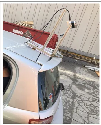
The hardware setup is mounted on the top of a car 2 m above the ground. The LiDAR and the camera are pointed toward the ground with an angle of 50 degrees. Both sensors cover a common 2 m x 4 m surface. The LiDAR scanning resolutions are 512 x 16 and 256 x 16 at 10 Hz and 20 Hz. The camera resolution is 1920 x1080 pixels at 120 frames per seconds. The car speed is up to 40 km per hour. Figure 2.5 shows the setup installed on the top of a car.
Figure 2.5 The LiDAR and the camera installed on the top of the car
CHAPTER 3
SELF-DRIVING CAR’S SENSORS: TESTS AND RESULTS
We conduct several experiments to test self-driving car’s sensors capability in detecting pavement distresses. We first run indoor experiments on the LiDAR to test its accuracy and resolution. Then, we test its capacity in detecting pavement elevation. Then a second experiment on the camera is conducted. We collect pavement videos and we test a Region-based Deep Neural network in detecting cracks.
In this chapter, we present the experiments conducted on self-driving car’s sensors, the results, and their interpretation.
3.1 Experiments on the LiDAR
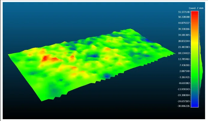
To test the LiDAR accuracy, we conduct indoor and outdoor tests. In the indoor tests, we evaluate the effect of the reflectivity of a scan: We scan a high reflective surface (i.e., a white board) and a low-high reflective surface (i.e., chess board) and we evaluate the performance of the LiDAR in both experiments. We set the LiDAR 1.6 m above the ground and we collect measurements at 10 frames per seconds. We use three methods to assess the LiDAR accuracy: in the first one, we measure the Euclidian distance between a reference and the measured point cloud; in the second, we measure the distance between the point cloud and the best fit plane; in the third, we reconstruct the surface from the scanned point cloud and we evaluate the surface elevation of the reconstructed 3D map. In the outdoor tests, we collect LiDAR data from a moving vehicle and we test the measured point clouds in different scenarios by reconstructing the pavement surface and evaluating its elevation.
The 3D measurements acquired from the LiDAR are in range format, i.e., the measurements represent how far is the LiDAR from the measurement point. To convert the measured range
into 3D coordinates we follow Equation 3.1 extracted from Ouster manual (Ouster, 2018): r is the measured range in mm, 𝜃 is the azimuth angle in radian, 90112 is the encoder ticks maximum number, φ is the beam altitude angle in radian, i is the number of channels (i.e., [1; 16]), x, y, and z are the 3D coordinates of the measured points. We use the 3D coordinates to generate a point cloud and compare it to a reference point cloud and a reference plane.
𝑟 = 𝑟𝑎𝑛𝑔𝑒 𝑚𝑚 𝜃 = 2𝜋 𝑒𝑛𝑐𝑜𝑑𝑒𝑟_𝑐𝑜𝑢𝑛𝑡 90112 φ = 2𝜋 𝑏𝑒𝑎𝑚_𝑎𝑙𝑡𝑖𝑡𝑢𝑑𝑒_𝑎𝑛𝑔𝑙𝑒𝑠[𝑖] 360 𝑥 = 𝑟 cos(𝜃) cos( φ) y = −r sin(𝜃) cos(φ) 𝑧 = 𝑟 𝑠𝑖𝑛(𝜑) (3.1) 3.1.1 Indoor Experiments
3.1.1.1 Cloud to Cloud/Mesh Distance
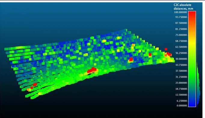
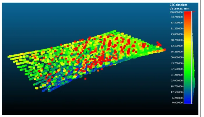
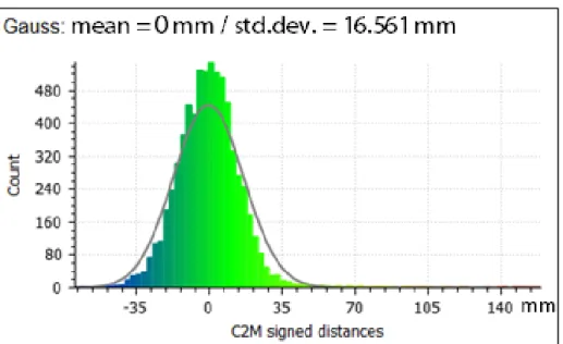
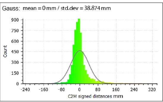
We create two indoor environments to test the accuracy of the LiDAR. In the first one, we scan a white board. By doing so we assess the accuracy of the scanned point cloud while scanning a surface with high reflectivity. In the second environment, we scan a mixed reflectivity board, Figure 3.1. We use CloudCompare software (CloudCompare, 2018) to measure the cloud to cloud (C2C) and cloud to mesh (C2M) distance to assess the accuracy of the LiDAR. C2C measures the distance between an input point in the point cloud and its nearest in the reference point cloud. C2M measures the distance between an input point in the point cloud and a mesh (plane surface). By computing the discrepancy between the scanned point cloud and its references we assess the accuracy of the LiDAR measurements.
Figure 3.1 Environment 2, surface with mixed reflectivity
The generated point clouds for both environments are shown in figures 3.2 and 3.3. To test the accuracy of the LiDAR, we compute the Euclidian distance between the generated point cloud and the reference point cloud, Figure 3.4. The reference point cloud is generated by simulating the LiDAR beams firing into a plane surface 1.6 m below the LiDAR. Equation 3.2 represents the parametric equation of the beams firing on a flat surface. This equation is obtained by calculating the trajectories that the LiDAR beams take while scanning a surface. The trajectories are based on the intersection of cones with a plane surface. The LIDAR position is the cone vertex. The variables in Equation 3.2 are defined as follows: x, y, and z are the 3D coordinates of the points in the reference point cloud. φ is a constant value that represents the LiDAR angle in which it is directed to the ground, d is a constant value that represents the sensor height to the ground. δ is the channel angle as defined in the data sheet of the sensor (i.e., δ has 16 angle values that represents the distribution of the laser beams inside the LiDAR), ANNEX II. And θ is the angle where the beam is fired (i.e., θ has 512 or 256 values depending on the vertical resolution of the scan), it varies between -90o and 90o with a fixed step (i.e., 0.7o
Figure 3.2 Environment 1, high reflectivity point cloud